Author Contributions
Conceptualization, V.S.P. and M.K.; methodology, V.S.P.; software, M.K.; validation, M.K. and V.S.P.; formal analysis, V.S.P., B.P. and N.N.; investigation, M.A. and V.S.P.; resources, B.P. and M.K.; data curation, N.N. and M.A.; writing—original draft preparation, M.K. and B.P.; writing—review and editing, V.S.P. and M.K.; visualization, M.A. and N.N.; supervision, V.S.P.; project administration, V.S.P.; funding acquisition, V.S.P. All authors have read and agreed to the published version of the manuscript.
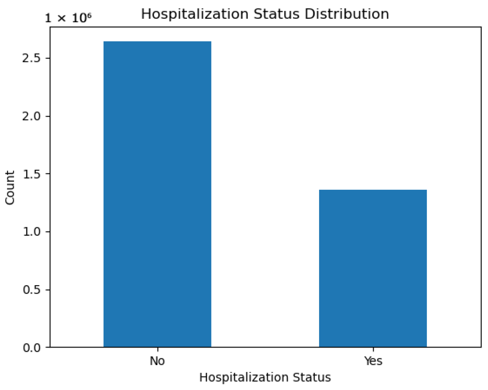
Figure 1.
Distribution of hospitalization status in the CDC dataset. Non-hospitalized cases dominate, motivating the use of imbalance-handling strategies.
Figure 1.
Distribution of hospitalization status in the CDC dataset. Non-hospitalized cases dominate, motivating the use of imbalance-handling strategies.
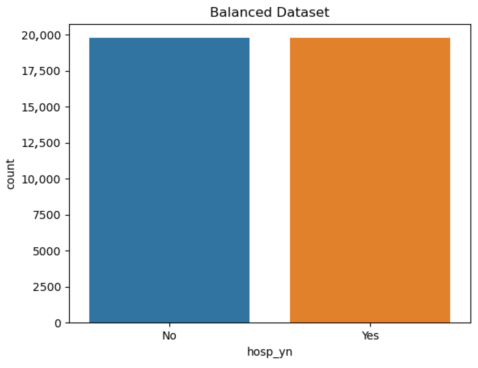
Figure 2.
Balanced dataset obtained after applying undersampling. The number of non-hospitalized (0) and hospitalized (1) cases was adjusted to achieve a 1:1 ratio.
Figure 2.
Balanced dataset obtained after applying undersampling. The number of non-hospitalized (0) and hospitalized (1) cases was adjusted to achieve a 1:1 ratio.
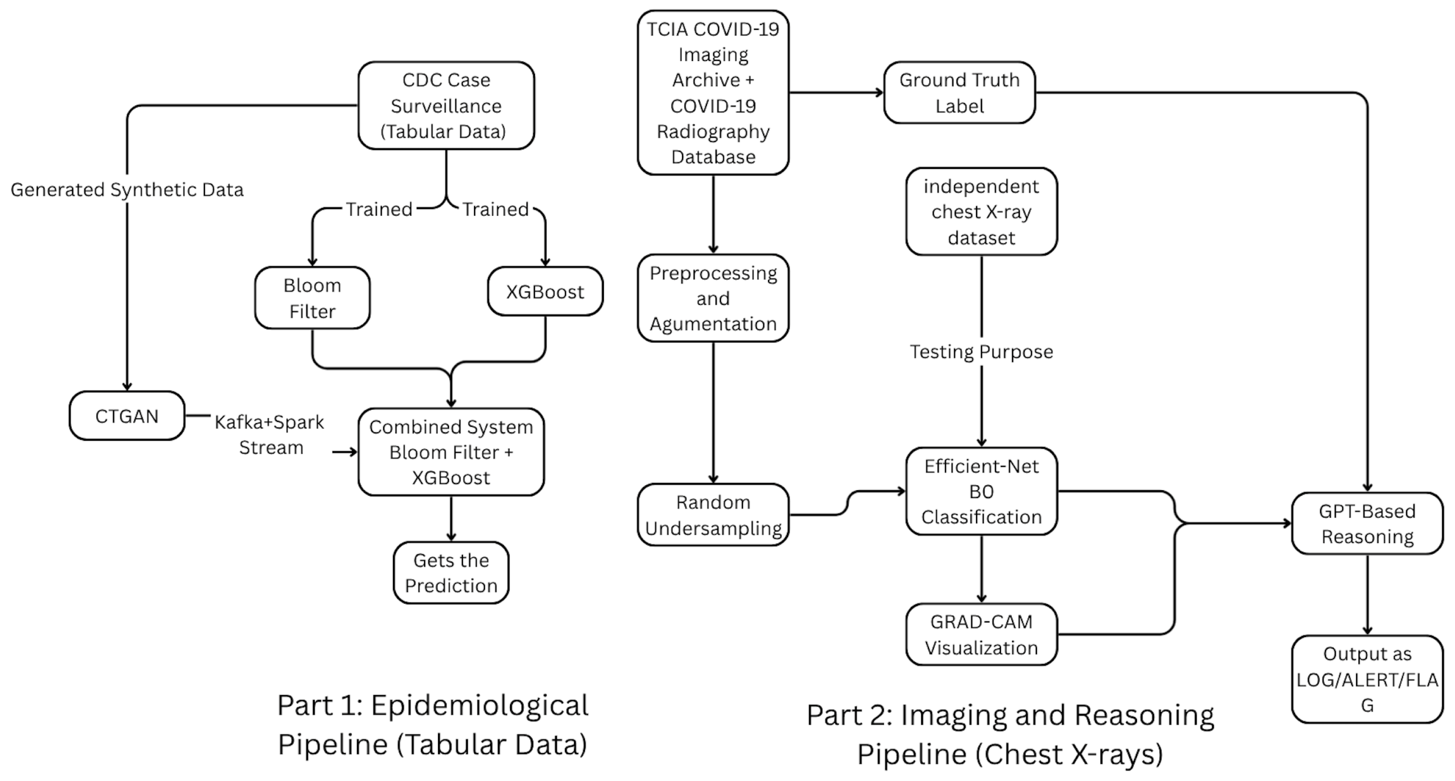
Figure 3.
Overall architecture of the dual big-data pipeline integrating (i) an epidemiological hospitalization-risk prediction module using CDC case-surveillance data and (ii) an imaging-based diagnostic reasoning module for chest X-rays. Both operate within a Kafka–Spark streaming framework, with CTGAN providing synthetic tabular data and a unified decision-logging layer consolidating predictions and auditable reasoning outputs.
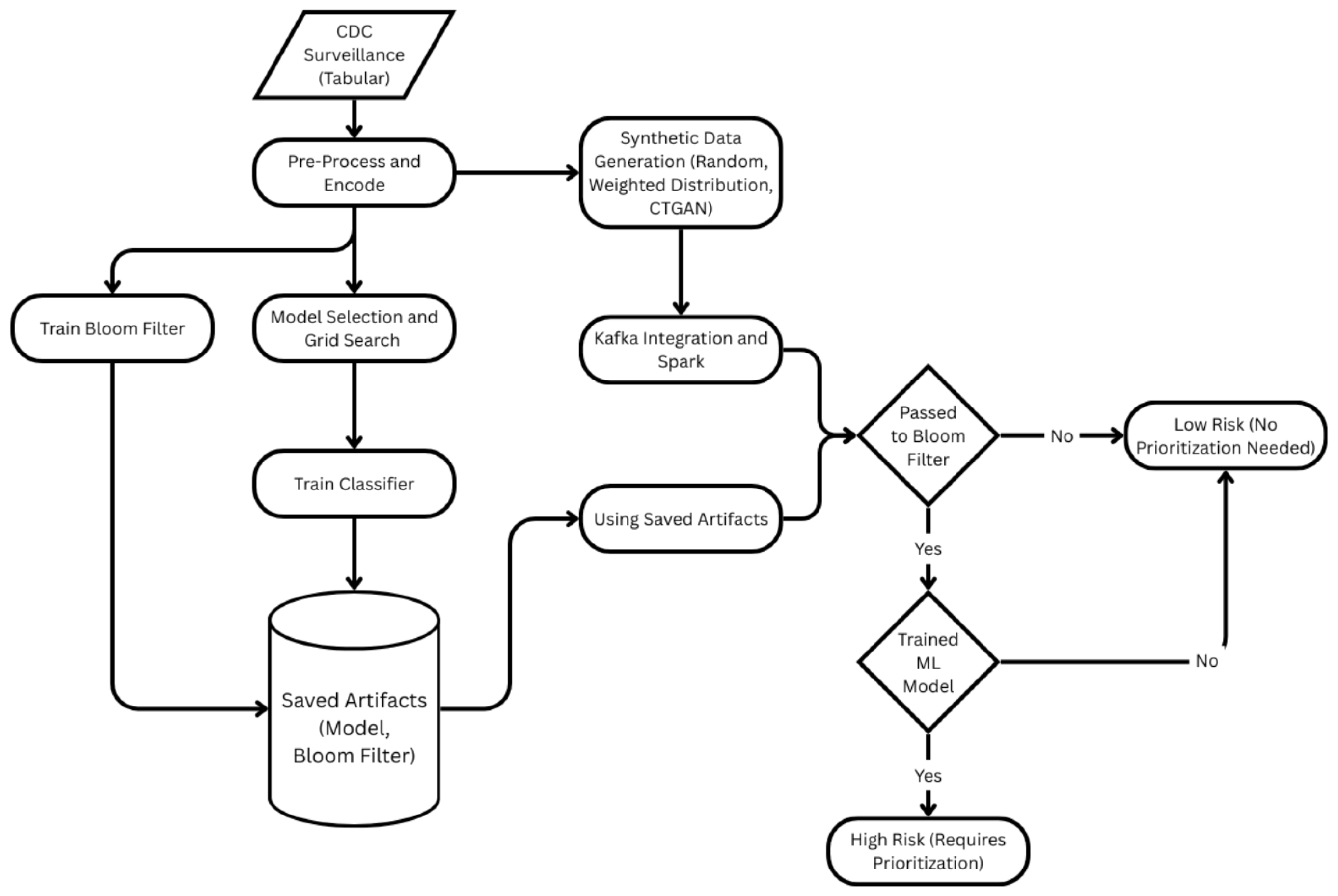
Figure 4.
Integrated surveillance data-based end-to-end pipeline for hospitalization risk at the patient level. Preprocessing/encoding, Grid Search model selection, XGBoost training, building a Bloom filter on high-risk profiles, and CTGAN-based synthetic generation are all included in the training path. To classify instances as Low-Risk or High-Risk (requiring priority), Kafka-Spark first ingests and encodes records, then conducts a Bloom-filter membership check and, if detected, scores using the learned model.
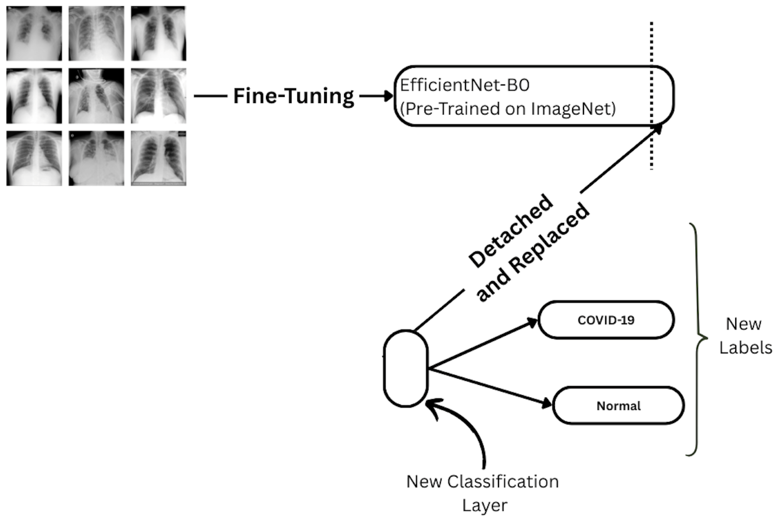
Figure 5.
Fine-tuning setup for EfficientNet-B0. The final classification head is detached and replaced with a new layer for binary prediction (COVID-19 vs. Normal).
Figure 5.
Fine-tuning setup for EfficientNet-B0. The final classification head is detached and replaced with a new layer for binary prediction (COVID-19 vs. Normal).
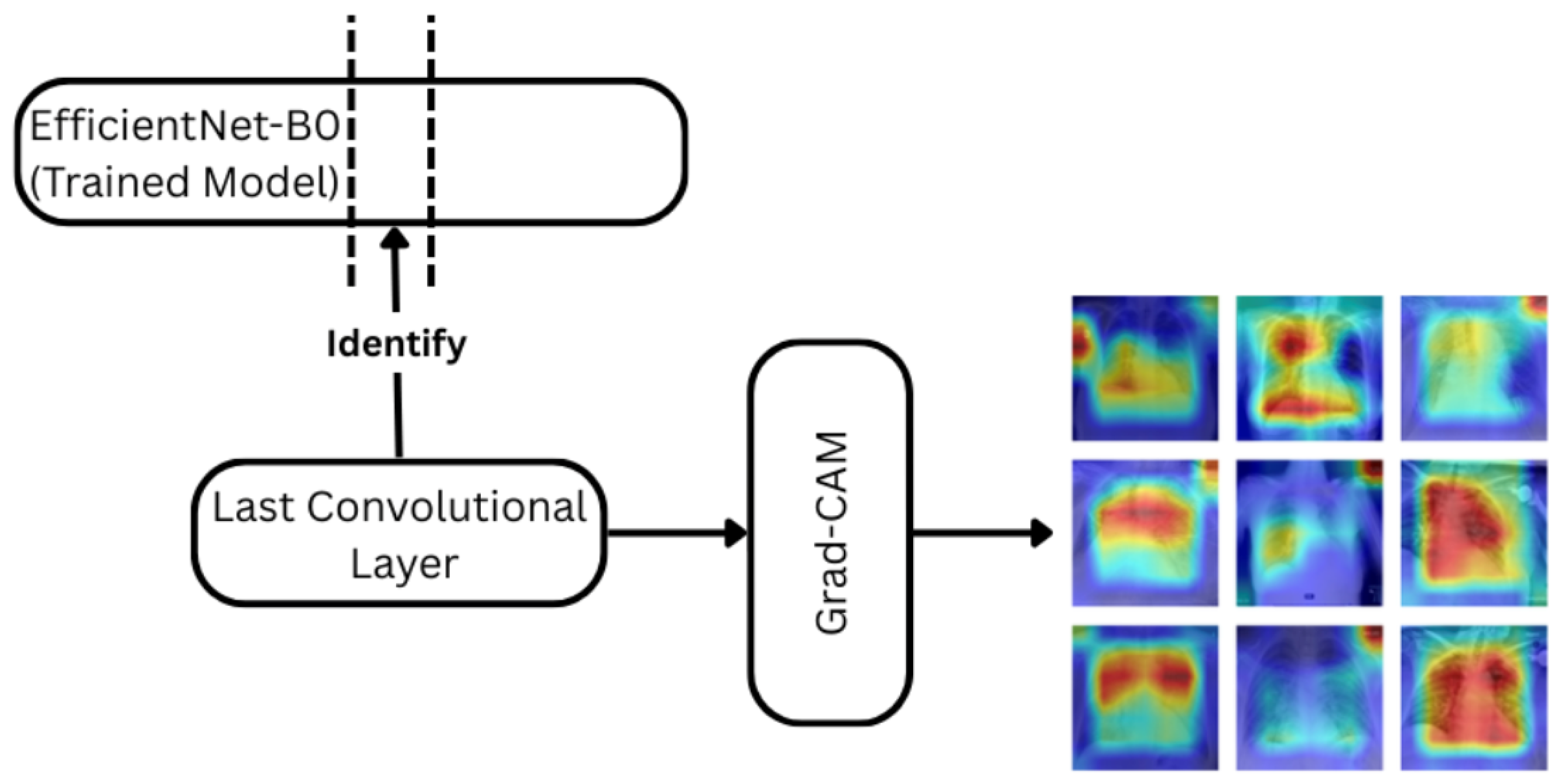
Figure 6.
Grad-CAM pipeline applied with the EfficientNet-B0 model trained. The penultimate convolutional layer is used to compute attention heatmaps for each prediction.The color gradients (red–yellow–blue) represent attention intensity, where red indicates regions of higher model focus and blue indicates lower attention.
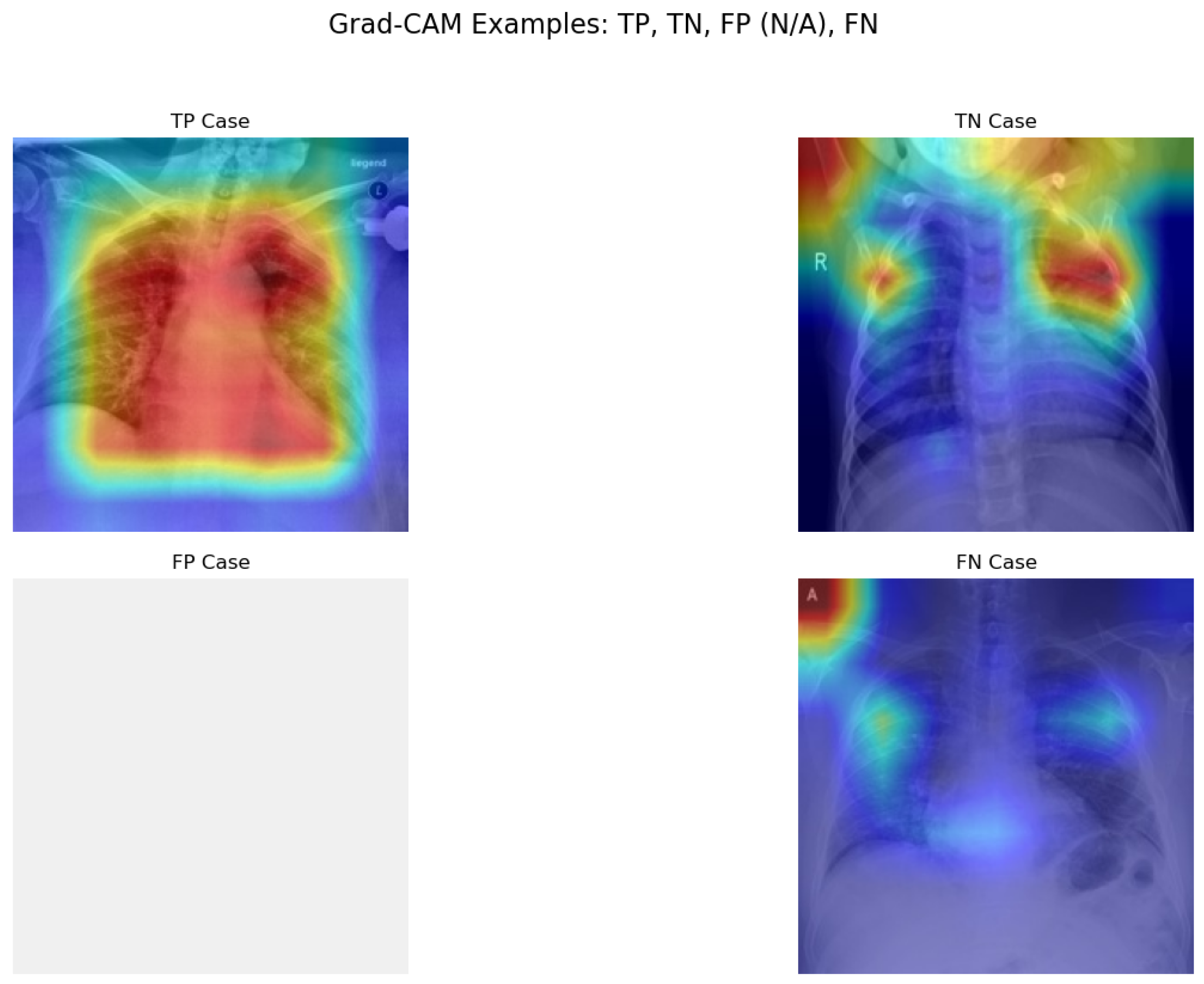
Figure 7.
Prototype Grad-CAM visualizations for TP, TN, and FN samples. The blank FP panel is intentional, as no false-positive cases occurred in this test set. Red/yellow areas indicate high model attention.
Figure 7.
Prototype Grad-CAM visualizations for TP, TN, and FN samples. The blank FP panel is intentional, as no false-positive cases occurred in this test set. Red/yellow areas indicate high model attention.
Figure 8.
ROC curves for Logistic Regression, Random Forest, and XGBoost. XGBoost shows the strongest trade-off between sensitivity and specificity.
Figure 8.
ROC curves for Logistic Regression, Random Forest, and XGBoost. XGBoost shows the strongest trade-off between sensitivity and specificity.
Figure 9.
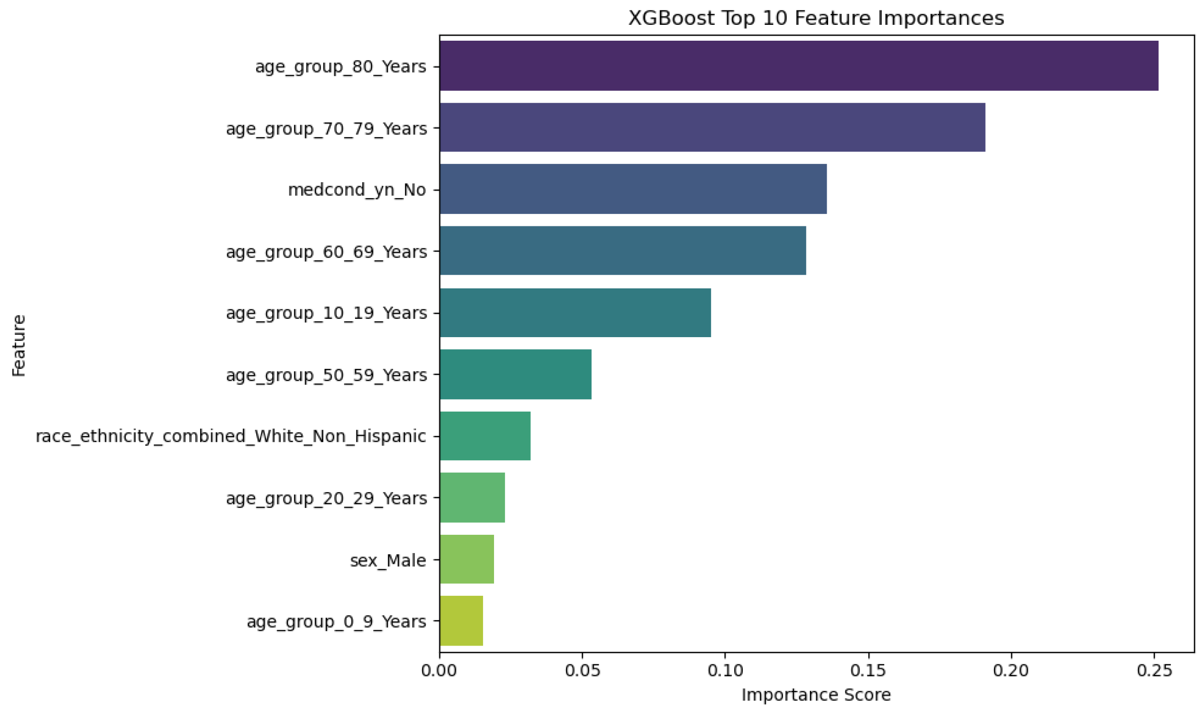
Top 10 Features and their Importance for XGBoost Model.
Figure 9.
Top 10 Features and their Importance for XGBoost Model.
Figure 10.
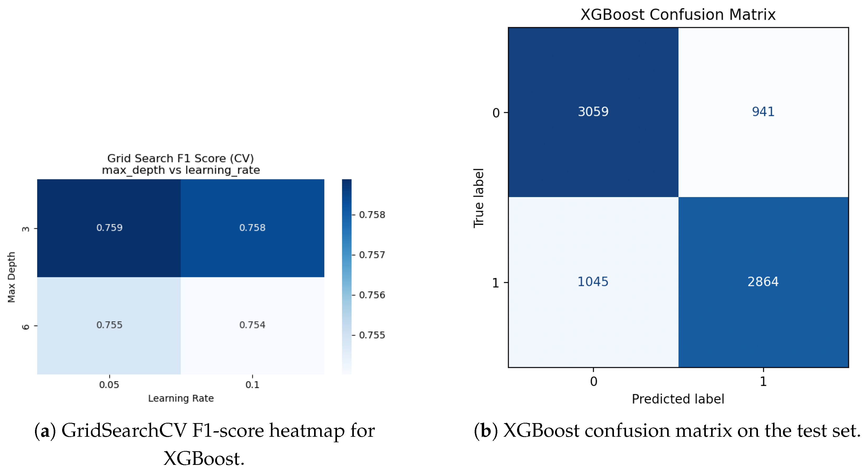
XGBoost hyperparameter adjustment and evaluation. Cross-validated F1-scores for various max_depth and learning_rate combinations are displayed in a heatmap (a). (b) The best XGBoost model’s confusion matrix on the held-out test set.
Figure 10.
XGBoost hyperparameter adjustment and evaluation. Cross-validated F1-scores for various max_depth and learning_rate combinations are displayed in a heatmap (a). (b) The best XGBoost model’s confusion matrix on the held-out test set.
Figure 11.
Comparison of class distributions generated by (a) Random, (b) Distribution-Aware, and (c) CTGAN approaches. CTGAN achieves the most balanced and realistic class proportions.
Figure 11.
Comparison of class distributions generated by (a) Random, (b) Distribution-Aware, and (c) CTGAN approaches. CTGAN achieves the most balanced and realistic class proportions.
Figure 12.
Comparison of class distributions generated by CTGAN at different training epochs. While 300 epochs show underfitting, 500 epochs provide the best balance and stability. Extending to 1000 epochs introduces signs of overfitting and instability.
Figure 12.
Comparison of class distributions generated by CTGAN at different training epochs. While 300 epochs show underfitting, 500 epochs provide the best balance and stability. Extending to 1000 epochs introduces signs of overfitting and instability.
Figure 13.
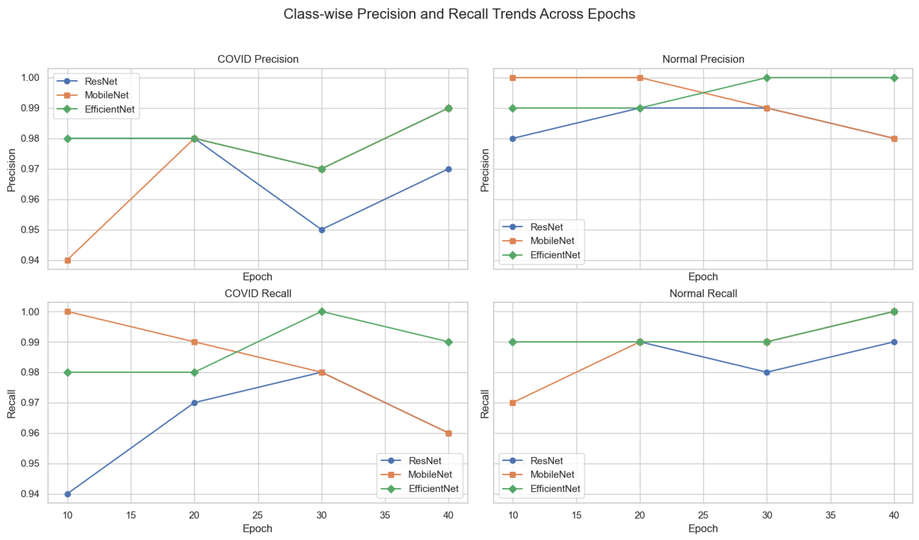
Class-wise precision and recall trends across training epochs for ResNet-18, MobileNetV2, and EfficientNet-B0. Each subplot isolates a specific metric and class, enabling detailed interpretation of model sensitivity and specificity over time.
Figure 13.
Class-wise precision and recall trends across training epochs for ResNet-18, MobileNetV2, and EfficientNet-B0. Each subplot isolates a specific metric and class, enabling detailed interpretation of model sensitivity and specificity over time.
Figure 14.
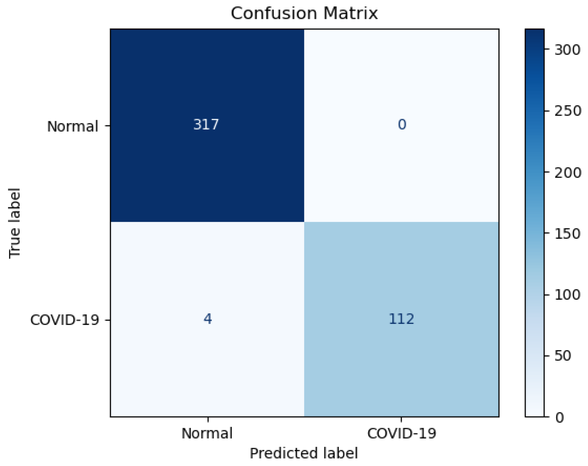
Confusion matrix for EfficientNet-B0 tested on an unseen test set.
Figure 14.
Confusion matrix for EfficientNet-B0 tested on an unseen test set.
Figure 15.
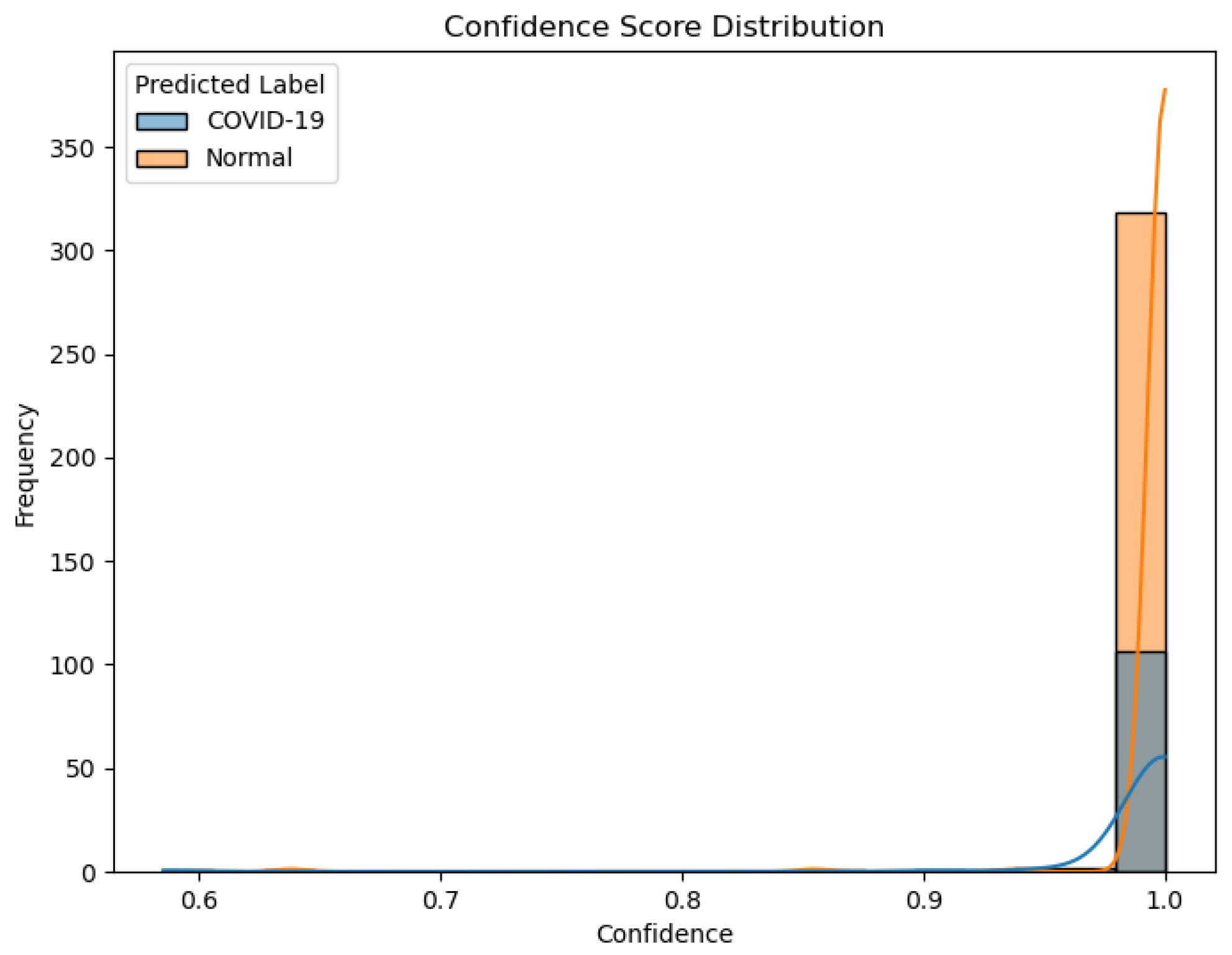
Confidence score distribution for predictions of EfficientNet-B0 on the unseen test set.
Figure 15.
Confidence score distribution for predictions of EfficientNet-B0 on the unseen test set.
Figure 16.
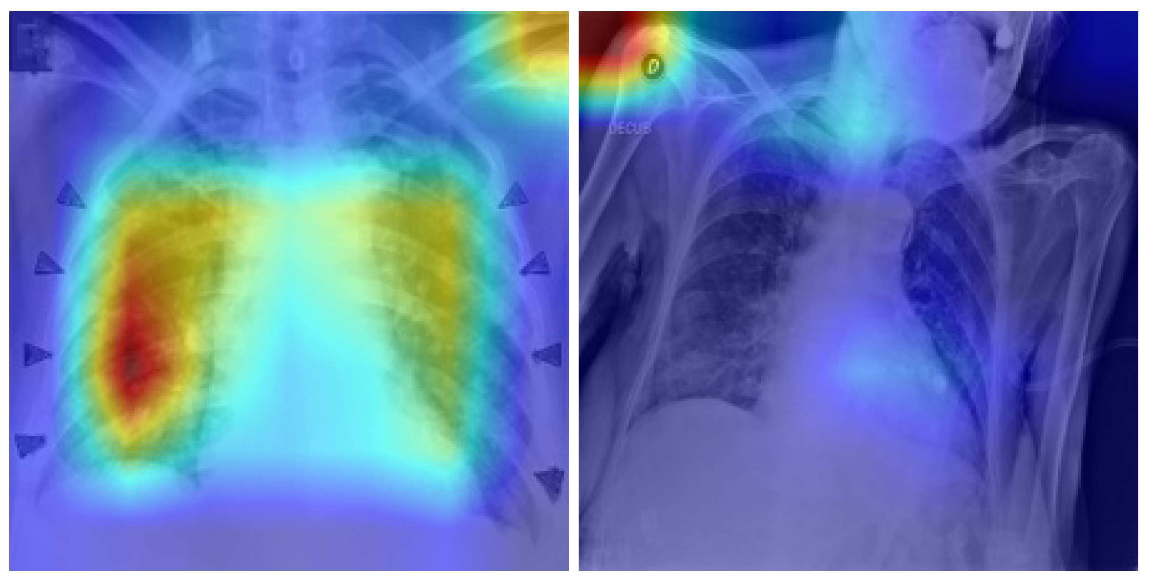
Grad-CAM attention patterns. (Left): Correctly classified COVID-19 case with strong activation in the bottom left lung, expected in healthy pathology. (Right): Incorrectly classified COVID-19 case (False Negative), where Grad-CAM attention is misplaced in irrelevant upper-body regions. Such visual misplacement indicates distraction or confusion by the model to irrelevant features. The color intensity (red = high model attention, blue = low attention) visualizes the regions influencing model prediction. Such visual misplacement indicates distraction or confusion by the model to irrelevant features.
Table 1.
Chest X-ray dataset composition before and after augmentation, and in the external test set.
Table 1.
Chest X-ray dataset composition before and after augmentation, and in the external test set.
| Category | After Merge (TCIA + Kaggle) | After Augmentation (Train) | External Test Set |
|---|
| Normal Images | 10,192 | 3000 | 317 |
| COVID Images | 3867 | 3000 | 116 |
| Total | 14,059 | 6000 | 433 |
Table 2.
Comparison of model performance across traditional and gradient-boosting classifiers for hospitalization risk prediction. All models show comparable accuracy and F1-scores, confirming XGBoost as the most balanced and practical choice for the streaming pipeline.
Table 2.
Comparison of model performance across traditional and gradient-boosting classifiers for hospitalization risk prediction. All models show comparable accuracy and F1-scores, confirming XGBoost as the most balanced and practical choice for the streaming pipeline.
| Model | Accuracy | F1-Score (No) | F1-Score (Yes) | Mean F1 |
|---|
| Logistic Regression | 0.75 | 0.75 | 0.75 | 0.75 |
| Random Forest | 0.75 | 0.76 | 0.74 | 0.75 |
| XGBoost | 0.75 | 0.75 | 0.76 | 0.75 |
| LightGBM | 0.75 | 0.76 | 0.75 | 0.75 |
| CatBoost | 0.75 | 0.75 | 0.74 | 0.75 |
Table 3.
Comparison of Bloom filter with XGBoost versus XGBoost alone (100,000 rows each iteration) in terms of execution time.
Table 3.
Comparison of Bloom filter with XGBoost versus XGBoost alone (100,000 rows each iteration) in terms of execution time.
| Iteration | Bloom + XGBoost (s) | XGBoost Only (s) |
|---|
| 1 | 9.52 | 9.90 |
| 2 | 9.04 | 9.12 |
| 3 | 9.88 | 9.35 |
| 4 | 9.31 | 9.70 |
| 5 | 9.22 | 9.28 |
| 6 | 9.46 | 10.12 |
| 7 | 9.19 | 9.21 |
| 8 | 9.85 | 9.14 |
| 9 | 9.28 | 9.74 |
| 10 | 9.36 | 9.42 |
Table 4.
Performance comparison of deep learning models across training epochs.
Table 4.
Performance comparison of deep learning models across training epochs.
| Model | Epoch | Accuracy | COVID F1-Score | Normal F1-Score |
|---|
| ResNet-18 | 10 | 97.8% | 0.96 | 0.98 |
| | 20 | 98.5% | 0.97 | 0.99 |
| | 30 | 97.9% | 0.96 | 0.98 |
| | 40 | 98.1% | 0.96 | 0.99 |
| MobileNetV2 | 10 | 98.1% | 0.97 | 0.99 |
| | 20 | 99.1% | 0.98 | 0.99 |
| | 30 | 98.6% | 0.98 | 0.99 |
| | 40 | 98.5% | 0.97 | 0.99 |
| EfficientNet-B0 | 10 | 98.8% | 0.98 | 0.99 |
| | 20 | 99.1% | 0.98 | 0.99 |
| | 30 | 98.7% | 0.98 | 0.99 |
| | 40 | 99.5% | 0.99 | 0.99 |
Table 5.
Classification report of EfficientNet-B0 on the unseen test set.
Table 5.
Classification report of EfficientNet-B0 on the unseen test set.
| Class | Precision | Recall | F1-Score | Support |
|---|
| Normal | 0.99 | 1.00 | 0.99 | 317 |
| COVID-19 | 1.00 | 0.97 | 0.98 | 116 |
| Avg/Total | 0.99 | 0.99 | 0.99 | 433 |
Table 6.
Quantitative summary of GPT-based reasoning outcomes on the external test dataset and their corresponding model confidence values.
Table 6.
Quantitative summary of GPT-based reasoning outcomes on the external test dataset and their corresponding model confidence values.
| Decision Type | Count | Percentage | Mean Confidence |
|---|
| LOG | 317 | 73.27% | 0.998 |
| ALERT | 112 | 25.81% | 0.993 |
| FLAG | 4 | 0.92% | 0.872 |
