Article

Algorithmic Investigation of Complex Dynamics Arising from High-Order Nonlinearities in Parametrically Forced Systems

1
Department of Mathematical Sciences, University of Engineering and Technology, Taxila 47050, Pakistan
2
IT4Innovations, VSB—Technical University of Ostrava, 708 00 Ostrava-Poruba, Czech Republic
3
Center for Theoretical Physics, Khazar University, 41 Mehseti Str., Baku AZ1096, Azerbaijan
*
Author to whom correspondence should be addressed.
Algorithms 2025, 18(11), 681; https://doi.org/10.3390/a18110681 (registering DOI)
Submission received: 29 August 2025 / Revised: 21 October 2025 / Accepted: 23 October 2025 / Published: 25 October 2025

Abstract

The geometric content of chaos in nonlinear systems with multiple stabilities of high order is a challenge to computation. We introduce a single algorithmic framework to overcome this difficulty in the present study, where a parametrically forced oscillator with cubic–quintic nonlinearities is considered as an example. The framework starts with the Sparse Identification of Nonlinear Dynamics (SINDy) algorithm, which is a self-learned algorithm that extracts an interpretable and correct model by simply analyzing time-series data. The resulting parsimonious model is well-validated, and besides being highly predictive, it also offers a solid base on which one can conduct further investigations. Based on this tested paradigm, we propose a unified diagnostic pathway that includes bifurcation analysis, computation of the Lyapunov exponent, power spectral analysis, and recurrence mapping to formally describe the dynamical features of the system. The main characteristic of the framework is an effective algorithm of computational basin analysis, which is able to display attractor basins and expose the fine scale riddled structures and fractal structures that are the indicators of extreme sensitivity to initial conditions. The primary contribution of this work is a comprehensive dynamical analysis of the DM-CQDO, revealing the intricate structure of its stability landscape and multi-stability. This integrated workflow identifies the period-doubling cascade as the primary route to chaos and quantifies the stabilizing effects of key system parameters. This study demonstrates a systematic methodology for applying a combination of data-driven discovery and classical analysis to investigate the complex dynamics of parametrically forced, high-order nonlinear systems.

1. Introduction

Nonlinear oscillations have a core role in promoting the study of dynamical processes in physics, engineering, and applied sciences. They are discrete in contrast to the linear systems, which respond in a proportional manner to the input, but nonlinear systems exhibit amplitude-dependent oscillations, bifurcation, and chaotic regimes that defy traditional analysis.
The prevalence of such behavior is manifested in a broad variety of real world systems. The complex nonlinear behavior of civil engineering structures like suspension bridges and high-rise buildings is exhibited by wind or seismic vibrations or excitations on the building structure [1,2]. Likewise, nonlinear electronic networks such as the oscillator of Chua’s, Van der Pol circuits, and radio frequency devices are also chaotic and have been used in the technologies of secure communication, random number generation, and signal processing technologies [3,4]. Nonlinear dynamics control processes in biological systems, such as neural synchronization in brain networks, cardiac oscillations, and arrhythmias [5]. The use of nonlinear approaches in control and mechanical engineering is necessary to stabilize and regulate highly complex systems in robotics, automotive suspensions, and aerospace structures [6,7], where the linear approach to modeling is not applicable due to nonlinearity in these systems.
The science of the nonlinear oscillations has developed in the past one hundred years by a number of achievements. The Mathieu equation, introduced in the 19th century, was the first to study parametric resonance. This was followed by the addition of cubic nonlinearities with the Duffing oscillator, which has been used to explain hardening/softening stiffness and nonlinear resonance phenomena [8,9]. More recently, quintic nonlinearities have been added to model nonstandard materials, nano- and micro-architectures, and metamaterials with force–displacement responses that are no longer cubic in nature [10,11,12]. These nonlinearities of high order are not mathematical curiosities anymore; these are a crucial component of realistic modeling of contemporary engineering systems. This interdisciplinary applicability is also true in the field of applied physics, where such vibrations are fundamental in the study of the phenomena in nonlinear optics and magneto-mechanical systems [13]. Soliton propagation in optics [14] is directly modeled in high-order cubic–quintic models, and high-order cubic–quintic models are also needed to describe the intricate resonance and switching of micro- and nano-mechanical (MEMS/NEMS) devices [15]. This interdisciplinary importance points to the universality of nonlinear oscillatory systems.
Even though nonlinear oscillations apply in a very general way, a wide range of approaches to their analysis continues to be based on a linearization process or a perturbative expansion based on small numbers. Even when such approximations work well in other instances, they do not work with large oscillations, or where nonlinearities of high order are important. Cubic–quintic restoring force systems are particularly tricky, now exhibiting multi-stability, jump phenomena, and complicated approaches to chaos that are not modelable in the cubic-only duffing models [16]. Such behavior is likely to be found in real materials because of nonlinear elasticity or large deflections, and requires models with both cubic and quintic terms. Such higher-order effects also render the system much more sensitive to initial conditions and so with riddled or fractal basins of attraction and multiple coexisting attractors.
These contributions represent the fact that cubic–quintic frameworks are a frontier in the study of applied nonlinear dynamics. Cubic–quintic models have been used to design adaptive energy absorbers in nonlinear vibration suppression in metamaterials [17]. In MEMS/NEMS developments, it has been demonstrated that cubic–quintic nonlinearity is capable of controlling dynamic striction and pull-in instability [18]. In optics, cubic–quintic Schrodinger models have been used in the production of femtosecond solitons and mode-locked fiber lasers [19]. In addition, new bifurcations to chaos in nonlinear oscillators with parametric forcing are studied in recent bifurcation analyses, especially in aerospace and energy systems [20,21,22].
The Mathieu and Duffing oscillators are the classical basis of the nonlinear vibration theory, with the former describing parametric stability and the latter introducing nonlinear restoring forces. Their generalization, the damped Mathieu cubic–quintic Duffing oscillator (DM-CQDO), includes increased nonlinearities as well as damping and is the new model of reference in the study of nonlinear dynamics. They have many approaches to their analysis. Harmonic balance and variants of Newton give true periodic approximations to higher orders [23], with homotopy and perturbation methods extending beyond the reach of standard perturbation [24,25], respectively. Strongly nonlinear oscillations have been captured using He’s energy balance method [26]. The numerical continuation methods allow one to track systematic second-order bifurcations and stability limits [27], whilst computational methods, such as finite element calculations, have been used on practical problems, such as bifurcations in brake squeal suppressions, photoelastic action in semiconductors, and axially moving beams [28,29,30].
In recent years, the algorithmic discovery of nonlinear dynamics has evolved rapidly through the integration of sparse regression and machine learning techniques. Beyond the original SINDy framework, numerous extensions have emerged, such as SINDy-PI for implicit systems [31], SINDy with control for feedback-driven models [32], and hybrid data-driven–physics-informed methods for noisy environments [33]. Although machine learning methods such as physics-informed neural networks (PINNs) and Koopman operator-based frameworks have recently been applied to nonlinear oscillators [34,35], these approaches often face important limitations. PINNs are capable of universal approximation, though they usually need large amounts of training data, hyperparameter optimization, and are computationally expensive. Koopman operator techniques offer a linear representation of nonlinear dynamics but can eliminate physical interpretability and require large-scale data to be accurately represented.
In contrast, SINDy directly yields sparse, interpretable governing equations with minimal data requirements, enabling a transparent link between the dynamics identified and the physical mechanisms. Chemical oscillations, particularly the Belousov–Zhabotinsky reaction [36], exhibit rich temporal patterns that are paradigmatic examples of nonlinear chemical dynamics and serve as models for biochemical oscillators. Other studies have been able to model this reaction based on experimental measurements, and on recurrence analysis, but in our case, we used the sparse regression (SINDy) on noisy discretization of the time-dependent mechanics of a mechanical oscillator. Both methods seek to discover low-dimensional interpretation of complicated dynamics; however, they differ in information and model systems. The efficiency and interpretability of the SINDy method is especially useful in the analysis of mechanical oscillators with nonlinearities of high order.

1.1. The Damped Mathieu Cubic–Quintic Duffing Oscillator

In order to respond to these dynamics, in this research, DM-CQDO, a damped parametrically forced and high-order nonlinear model, is used. Physically, this model represents a mass-spring-damper system mounted on a vibrating base, as shown in Figure 1.
The mechanical elements represented in Figure 1 represent the terms of the equation that describes the system. The inertia of the mass gives rise to the second-order term ( Z ¨ ). The damper generates a dissipative force that is dependent on velocity, and it is shown by the damping term ( Γ Z ˙ ). The nonlinear spring restoring force consists of a linear stiffness component ( η Z ), a cubic term ( Ξ Z 3 ), and a quintic term ( ϕ Z 5 ). Lastly, the vibrating base motion also adds a time-varying modulation of spring stiffness, which is represented by the parametric excitation term of the spring ( ζ cos ( Ω t ) Z ). This is the parametric excitation, a general stimulus that motivates the system into the complicated resonant and chaotic states. This relationship between the physical system and its mathematical representation is formally expressed by the DM-CQDO equation:
Z ¨ + Γ Z ˙ + [ η + ζ cos ( Ω t ) ] Z + Ξ Z 3 + ϕ Z 5 = 0 .
A systematic summary of these parameters and their physical interpretations is provided in Table 1.
To facilitate numerical and analytical treatment, Equation (1) is reformulated as an equivalent first-order system of ordinary differential equations. Let y 1 = Z , y 2 = Z ˙ , and y 3 = Ω t , where y 2 denotes the velocity, and y 3 tracks the excitation phase. Substituting these definitions into Equation (1) yields the following:
d y 1 d t = y 2 , d y 2 d t = γ y 2 n 1 2 q cos ( y 3 ) y 1 L y 1 3 M y 1 5 , d y 3 d t = δ .
This formulation reveals how damping, parametric excitation, and nonlinear stiffness jointly influence the system’s motion. The first-order representation preserves the physical interpretation of the original DM-CQDO while enabling efficient numerical integration and standard dynamical analysis such as bifurcation, Lyapunov, and basin studies.

1.2. Research Gaps and Contributions

Although extensive research has been conducted on the dynamics of nonlinear systems, a closer examination of the literature reveals several research gaps:
  • Most existing work does not explicitly employ a comprehensive suite of established chaos detection techniques to fully characterize the dynamical behavior of complex nonlinear oscillators.
  • Many studies assume a perfectly known model, often overlooking the application of modern data-driven methods to discover the governing equations of such oscillators from time-series data alone.
  • While bifurcation behavior is often discussed, a systematic and quantitative analysis of how parameters like damping control the various routes to chaos is not always present.
The primary contribution of this work is not the development of new individual algorithms, but rather the demonstration of a unified workflow that integrates modern data-driven model discovery with a full suite of classical chaos diagnostics, providing a clear path from time-series data to physical insight. To this end, our contributions are as follows:
  • We present the first comprehensive stability diagram for the DM-CQDO in the forcing amplitude and frequency parameter space, clearly mapping the boundaries between periodic, quasiperiodic, and chaotic regimes.
  • We identify the period-doubling cascade as the primary route to chaos and quantitatively demonstrate how its onset is controlled by the systems damping coefficient through a detailed bifurcation analysis.
  • Through a data-driven discovery framework, we validated the governing equations and confirmed the dominant influence of the cubic nonlinearity and the parametric forcing terms in shaping the system’s complex dynamical response.
  • We also performed a careful study of the inherent multi-stability of the system with the aid of quantitative Lyapunov analysis and graphical constraints of the fractal organization of attractor basin boundaries. Notably, the suggested workflow is not restricted to the DM-CQDO, which this research takes into consideration. All of these components, i.e., sparse model discovery, bifurcation analysis, Lyapunov exponent calculation, spectral diagnostics, recurrence mapping, and basin classification, have been formulated within a generalizable framework that can be readily applied to a wide range of nonlinear systems, such as electronic circuits, MEMS/NEMS, and biological oscillators. This building block architecture makes the method more reliable and adaptable, making it a general diagnostic platform and not a case-specific procedure.
This manuscript is reorganized to make the presentation as clear as possible and to increase the logical flow of the presentation. The updated version starts with the empirical finding of the governing equations (Section 2), then systematic bifurcation and stability analysis (Section 3), attractor geometry investigation (Section 4), and frequency-domain diagnostics (Section 5). This chronological structure—model identification and qualitative and quantitative characterization—provides a logical flow of this paper and emphasizes the originality of the provided structure as the full-fleet diagnostic pipeline to work with such a complex nonlinear system.

2. Identifying the System Dynamics

This section details the application of the SINDy algorithm. The objective is to verify that SINDy could accurately reconstruct the oscillator’s governing equation by analyzing its simulated behavior over time.

2.1. Algorithm

The Sparse Identification of Nonlinear Dynamics (SINDy) algorithm is a data-driven algorithm that predicts the equations of motion of a dynamical system based on available time-series data of the system itself directly. In this research, the method is applied in a step-by-step process that follows the following steps:
  • Data collection: First, time-series data for the system’s state variables are collected. For a system with states y ( t ) = [ y 1 ( t ) , y 2 ( t ) , , y n ( t ) ] , we form a data matrix Y . The time derivatives y ˙ ( t ) are also required and are typically computed numerically from the data, forming a derivative matrix Y ˙ .
  • Candidate function library construction: A library, Θ ( Y ) , of candidate nonlinear functions is constructed. This library contains potential terms that might appear in the governing equations. In the case of the oscillator analysis, the library of candidate functions was built to contain both the poly terms (e.g., y 1 , y 1 2 , y 1 3 , y 1 5 ) and the trigonometry terms (e.g., cos ( y 3 ) , y 1 cos ( y 3 ) ) by making sure the basis functions capture the necessary nonlinear and parametric characteristics of the system.
  • Sparse regression: The core of SINDy is solving the linear system Y ˙ = Θ ( Y ) Ξ for the coefficient matrix Ξ . Crucially, SINDy assumes that the governing equations are sparse, meaning only a few terms in the library are active. To find this sparse set of coefficients, we employed the sequentially thresholded least-squares (STLSQ) algorithm. This iterative method solves for Ξ and then sets any coefficients with a magnitude smaller than a predefined threshold to zero, repeating until the solution converges.
  • Model reconstruction: The non-zero values of coefficient matrix Ξ determine the active terms of the system. This choice provides a set of differential equations and is short and open to interpretation; further, this choice best describes the behavior found in the data.

2.2. System Simulation

The investigation was initiated using the known ground-truth model, formulated as a system of nonlinear ordinary differential equations:
d y 1 d t = y 2 , d y 2 d t = y 1 0.2 y 2 0.1 y 1 3 0.01 y 1 5 + y 1 cos ( y 3 ) , d y 3 d t = 1 .
Though the damped and modulated cubic–quintic Duffing oscillator (DM-CQDO) is employed in this case as an illustrating example, the workflow is model-independent, as only time-series data are required as input. This renders the same identification strategy to be generalized to other nonlinear oscillators or experimental data. Time interval t [ 0 , 100 ] was simulated with a nominal time step of Δ t = 0.01   using an initial condition of y 0 = [ 2 , 0 , 0 ] T . This initial condition was chosen to make sure that the nonlinear modes are sufficiently excited so that the whole behavior of the system could be identified. The output of the SINDy algorithm was the resulting trajectory.
To check the numerical accuracy, the equations were integrated by the fourth-order Runge–Kutta (RK4) method and adaptive step sizes with Δ t = 0.005 to 0.02 were used. Common phase-space trajectories, the same bifurcation structures, and the same estimates of the Lyapunov exponents were found with all the measured step sizes. Moreover, the total energy change was less than 10 4 per iteration, which means the simulations were not affected by the numerical effects. These tests help verify that the time stepping and integration method used gives sound and stable results to all dynamical regimes studied.

2.3. Model Identification and Comparison

Using this simulated trajectory as input, we applied the SINDy algorithm, which performs a sparse regression on a library of candidate functions to find the most parsimonious model describing the dynamics. We employed the sequentially thresholded least-squares algorithm (STLSQ) in SINDy, where coefficients below a fixed threshold are set to zero and the regression is iterated until convergence. This fast truncation-based method performed well for our system; alternative sequential elimination approaches may be preferable for partially observed or highly scale imbalanced systems. The algorithm successfully identified the following governing equations:
d y 1 d t = y 2 , d y 2 d t = 0.9801 y 1 0.1696 y 2 0.1092 y 1 3 0.0012 y 1 5 + 0.9480 y 1 cos ( y 3 ) 0.0142 cos ( y 3 ) , d y 3 d t = 1 .
A direct comparison between the true and identified coefficients is presented in Table 2. The parameters show excellent agreement with the true values, with minor deviations attributable to numerical differentiation and regression trade-offs. A recent SINDy extension promotes global stability by constraining quadratic models with Lyapunov conditions. Since our system includes cubic and quintic terms, this method is not directly applicable, but similar ideas could be adapted in future work, especially for noisy experimental data.

2.3.1. Phase Analysis

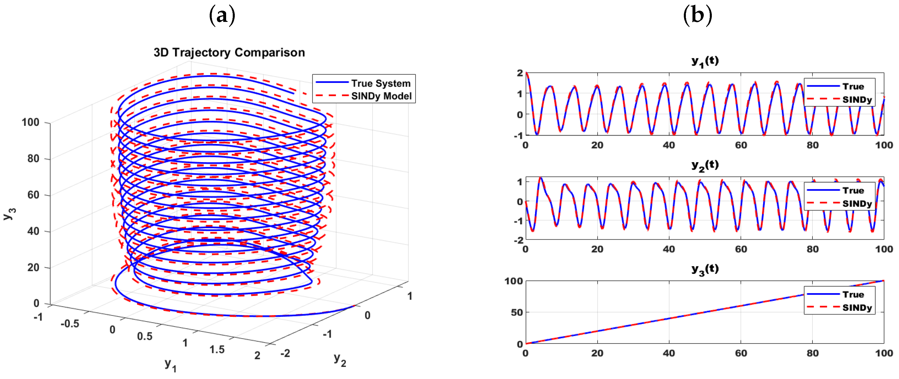
The 3D phase trajectories of both the true system and the SINDy identified model are displayed in Figure 2a. The plot clearly shows that the discovered model’s trajectory almost perfectly overlays the true trajectory, indicating that the algorithm has successfully captured the system global dynamics and the geometry of its attractor.

2.3.2. Time-Series Fidelity

Figure 2b provides a quantitative, time-domain comparison of each state variable. The time series for y 1 ( t ) , y 2 ( t ) , and y 3 ( t ) of the identified model are plotted against the ground truth. The near-perfect overlap between the true and predicted signals confirms the high fidelity of the discovered model.
It is very evident that the identification model is effective due to the high level of congruence between the original system and the identified model numerically tested in Table 2 and visually in Figure 2. The approach was able to reconstruct the underlying structure of the complex nonlinear dynamics, resulting in a mathematical model that was precise and physically interpretable.

3. Global Behavior and Stability Analysis

3.1. Bifurcation Analysis

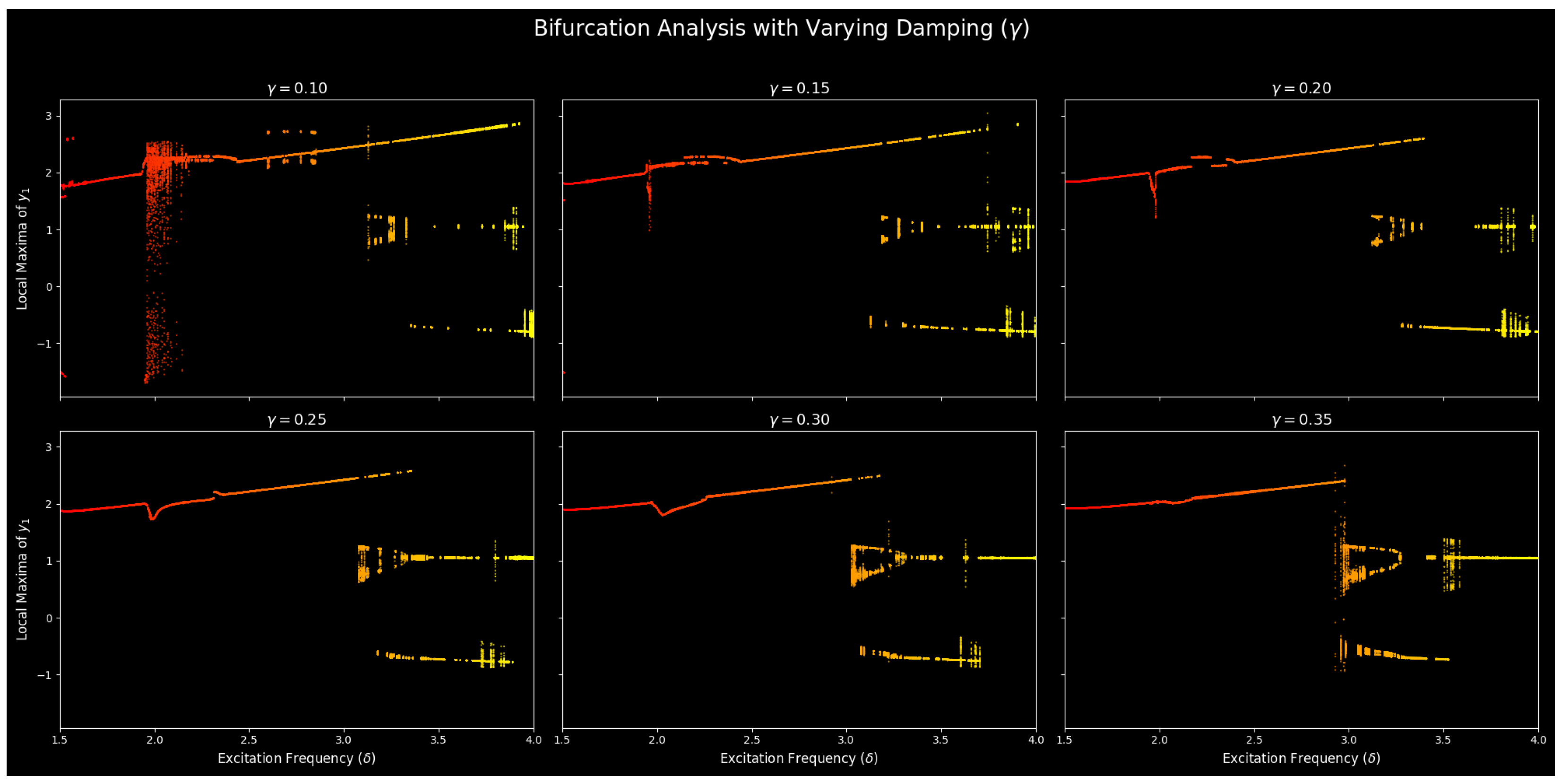
To investigate how the system evolves into a chaotic system, a bifurcation analysis was performed. The method defines the long-term dynamical states of the system with one of the most important control parameters changed. The frequency of excitation ( δ ) was experimentally manipulated in this experiment at a constant damping coefficient ( γ ). Figure 3 illustrates the resulting bifurcation diagrams. An evident trend is observed out of these results: a gradual raise in the damping coefficient ( γ ) levels the oscillator. Because the excitation frequency increases, the bifurcation point changes, and a higher frequency causes a bifurcation point at the lower panel (see Figure 1). It is necessary that ( δ ) will push the system out of periodic motion into chaos as the damping becomes stronger. For instance, when γ = 0.10 , chaos emerges at δ 1.8 , whereas at a high damping of γ = 0.35 , the system remains stable until δ 3.6 . Table 3 summarizes this stabilizing effect of damping quantitatively. The specific path to chaos can also be seen in the bifurcation diagrams. Specifically, the panel of the correspondence to ( δ ) can be seen. The characteristic features of a period-doubling cascade, which is one of the most known ways to chaotic behavior, can be seen in 0.25. As ( γ ) grows larger than 3.2 and the single branch of the period-1 orbit bifurcates to form two (period-2), then four (period-4), and so on, a fully aperiodic regime is reached. This discussion establishes that the period-doubling cascade is the leading process that causes chaos to occur in the system.

3.1.1. General Trend: The Stabilizing Effect of Damping

A panel of six bifurcation diagrams is shown in Figure 3 below, where the values of the damping coefficient ( γ ), are fixed to different values. One of the most obvious and dramatic tendencies can be observed at a glance through a comparative analysis of the plots, which is the systematic stabilization of the system by increasing the damping coefficient γ . This stabilization is observed through slowing down of the complex behaviors; the larger the γ , the larger the excitation frequency δ needed to take the system out of a simple periodic motion into chaos.

3.1.2. Detailed Analysis of Dynamic Regimes

The specific characteristics of the transition to chaos are highly dependent on the level of damping. We can distinguish between three primary modes of behavior observed in the analysis.
  • Case 1: Low amplitude ( γ = 0.10 , 0.15 ): At low damping values (e.g., γ = 0.10 and γ = 0.15 ), the system suddenly and almost explosively switches to broadband chaotic behavior at a comparatively low excitation frequency ( δ 1.8 ). The resulting chaotic attractor is of a large range of y 1 values. The parametric forcing is easily capable of injecting enough energy to overcome the restoring forces of the system with minimal energy dissipation, to permit the trajectories to explore a very large, complex region of phase space and support very high-amplitude chaotic oscillations.
  • Case 2: Moderate amplitude ( γ 0.25 ): For the diagram for γ = 0.25 , the system is known to undergo a canonical period-doubling cascade, a familiar cause of chaos. At first, there is a period-1 limit cycle. At a bifurcation point ( δ 3.2 ), as δ is exceeded, this orbit becomes unstable and forms a period-2 orbit, which is represented in the bifurcation diagram as the branching of one branch into two. Additional bifurcations of δ are successive bifurcations, with the period-2 orbit bifurcating into period-4, period-8, etc. This cascade proceeds until the number of periods essentially goes to infinity, at which point the system exhibits aperiodic chaotic behavior.
  • Case 3: High amplitude ( γ 0.30 ): With increased damping, the chaos transition is smoother and organized. To achieve a period-doubling cascade, the major route is still the period-doubling cascade, but it now begins with larger excitation frequencies ( δ ), and its overall extent of chaotic motion is smaller. This action underlines the stabilizing influence of the damping being enhanced that smothers the scale and the amount of the chaotic dynamics.

3.1.3. Quantitative Summary of Transitions

The graphical tendency of delayed chaos increasing damping in greater amounts is measured in Table 3. The table is a table of the approximate value of critical excitation frequency, δ c , at which chaotic behavior is first induced by the value of γ . This mathematical summary validates the idea that a fivefold increase in damping (0.15 to 0.35) will increase the δ value necessary to cause chaos by two times; therefore, the overall stability of the systems is highly predictable and depends on damping.

3.2. Stability Diagrams in the Parameter Space

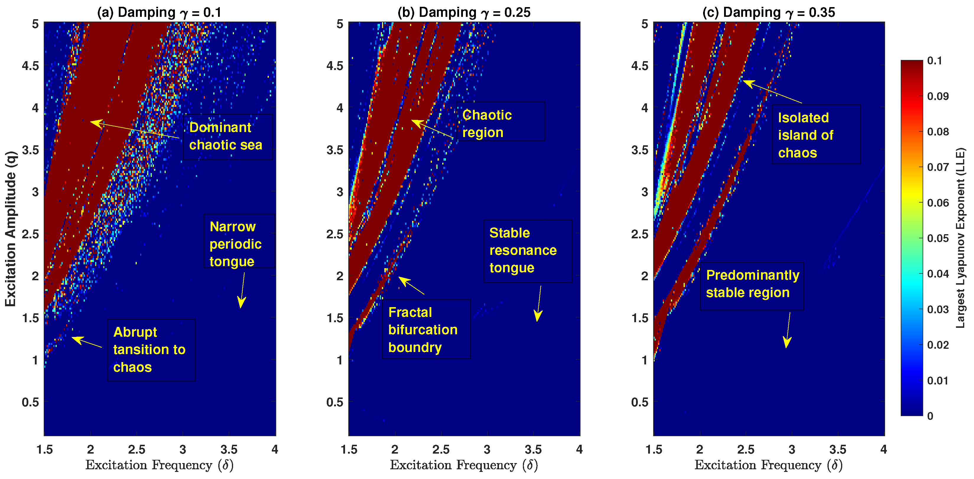
To provide a comprehensive overview of the DM-CQDO global dynamical behavior and to address the influence of damping, we constructed a series of stability diagrams in the parameter space spanned by the excitation frequency ( δ ) and the excitation amplitude (q). The results are presented in Figure 4 for three distinct damping coefficients: (a) low damping ( γ = 0.1 ), (b) intermediate damping ( γ = 0.25 ), and (c) high damping ( γ = 0.35 ). Each diagram was obtained after computing the largest Lyapunov exponent (LLE) on a fine grid of parameters. The color of every point on the map represents the value of the LLE, with warmer colors (red/yellow) representing chaotic behavior (LLE > 0) and darker ones (blue) representing periodic or stationary motion (LLE 0 or less). The comparison of the three panels shows the ultimate position of damping as a control parameter in the dynamics of the systems globally:
  • Case (a): Low damping ( γ = 0.1 ) At low damping, the parameter space is dominated by a vast dominant chaotic sea that emerges at even moderate excitation amplitudes. The regions of periodic behavior are confined to a narrow periodic tongue and are quickly overwhelmed by chaos as the forcing amplitude increases. This global view corresponds to the abrupt transition to chaos observed in the one-dimensional bifurcation diagram for low damping.
  • Case (b): Intermediate damping ( γ = 0.25 ) As damping increases, the chaotic region recedes significantly, and the stable resonance tongues become much larger and more clearly defined. This shows that a larger forcing amplitude is now required to induce chaos. Critically, the boundary between the chaotic and periodic regions is no longer simple; it is a sharp and complex fractal bifurcation boundary, representing the loci of the period-doubling bifurcations that lead to chaos.
  • Case (c): High damping ( γ = 0.35 ) At high damping, the system is almost entirely stable and predictable, with the parameter space being a predominantly stable region. Chaos has been strongly suppressed, now confined to small, isolated islands of chaos that only appear at very high forcing amplitudes.
Overall, this systemic analysis of several stability diagrams can be taken as a map of how the DM-CQDO can and does behave globally. It does not only establish the presence of chaos, but also offers a new insight of strength, namely that damping is an organizing principle, which orders the landscape of stability by inhibiting chaos and amplifying the areas of predictable, periodic behavior. This is a direct visualization and measurement of the stabilizing effect that has been previously measured in the one-dimensional bifurcation diagrams.

3.3. Lyapunov Exponent

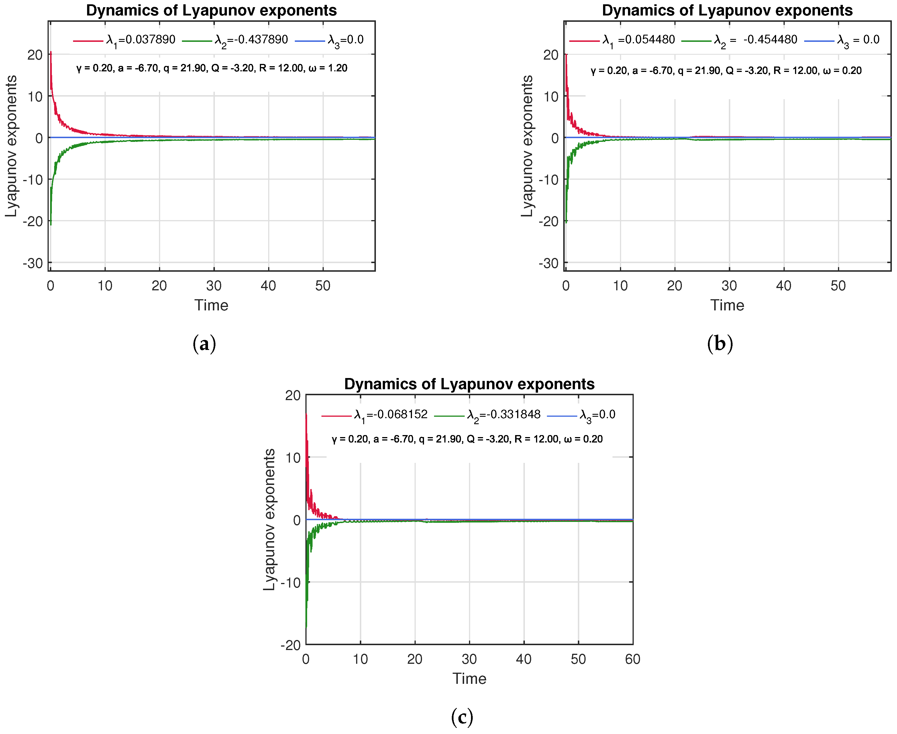
The bifurcation study has indicated a distinct shift between the stable and chaotic movement when the excitation frequency ( δ ) is changed. In order to measure this transition and observe the multi-stable behavior of the system, we have calculated the largest Lyapunov exponent ( λ 1 ). The case of ( λ 1 ) being positive is an unambiguous indicator of chaos, whereas a negative value would mean that it will converge to an attractor that is non-chaotic.
Three initial conditions were computed and the exponents of the initial conditions were determined using Gram–Schmidt reorthonormalization method [37] in order to probe the multi-stability of the system, as shown in Figure 5.
  • Case 1: Low-amplitude initial condition: In the first case of the condition (0.01, 0.01, 0.01), the maximum Lyapunov exponent is ( λ 1 = 0.033787 ). The positive value authenticates chaotic behavior, where small perturbations increase exponentially with time. Figure 5a indicates that the ( λ 1 ) is positive post initial transients, which proves the existence of a chaotic attractor.
  • Case 2: Medium-amplitude initial condition: Having the initial condition of medium amplitude (0.3, 0.3, 0.3), the system is more chaotic with a larger Lyapunov exponent ( λ 1 = 0.054480 ) (Figure 5b). This amplified value displays sensitivity to an initial condition and a more rapid separation of adjacent paths, indicating a stronger instability about this initial condition.
  • Case 3: High-amplitude initial condition: In the case of the high-amplitude initial condition (0.5, 0.5, 0.5), the largest Lyapunov exponent is negative, λ 1 = 0.068152 (Figure 5c) and the trajectories do tend to approach a non-chaotic, steady-state attractor. This constant reduction in the exponent by time, which is indicated by the figure, is a confirmation of the same result.
    Quantitative evidence of multi-stability is the existence of the positive and negative largest Lyapunov exponents, which are obtained using the same system parameters; the multi-stable dynamical system is one in which both chaotic and stable attractors appear at the same time.

3.4. Multi-Stability

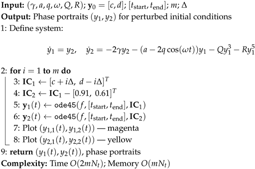
When multiple solutions exist at the same time in a nonlinear system, it is referred to as multi-stability. In these systems, small initial differences can ultimately result in major variations in how things develop long-term. The system is examined using the parameters γ = 0.07 , n 1 = 1.12 , q = 9.02 , δ = 2.092 , L = 0.001 , and M = 0.1 . Our approach is detailed in Algorithm 1. The initial conditions are changed to observe their effects on the system’s dynamical behavior. This examination demonstrates the presence of many attractors and reveals how differently the system can respond from different starting points.

3.4.1. Analysis Based on Figure 6

  • Figure 6a: This figure uses two initial conditions to show the difference between chaotic and periodic behaviors. The initial values for the first curve are ( y 1 , y 2 ) = ( 0.29 , 0.13 ) , and for the second curve they are ( y 1 , y 2 ) = ( 0.2 , 0.31 ) . The first curve shows very packed loops, while the second set of initial conditions results in regular, repeating loops that show stable oscillations. In time, both sets develop chaotic motion, revealing that small variations in the initial conditions greatly influence the system.
  • Figure 6b: A similar comparison between different attractors shows that the system still exhibits multi-stable behavior. With initial values of (0.3, 0.12), both periodic and chaotic behaviors are seen on the trajectory. When the system has multiple attractors, both orderly and disorderly regions begin to form, and the phase portrait explains how the system switches quickly between them.
  • Figure 6c: This is a different combination of initial conditions ( ( y 1 , y 2 ) = ( 0.329 , 0.10 ) ) used in Curve 1 and there is a displaced version in Curve 2. Both of the scenarios suggest that the system is sensitive to the initial data. Curve 1 represents bigger variations and distinct dispersion. Curve 2 starts off constrained but turns into a thicker structure, demonstrating how sensitive pushes may cause various attractor basins to emerge. This demonstrates that the further the initial conditions are displaced from the origin, less regularity is clear and there is more chaotic movement.
  • Figure 6d: This exploration is executed with a shift ω set to 0.4. The trajectories demonstrate that there is a greater difference between attractor behaviors. Curve 1 (coral) has a wide multi-lobed attractor, which is folded. Curve 2 (olive) begins as periodic, but then moves on to be a distinct chaotic attractor. A pair of different orbits in the phase space shows that there are two chaotic attractors of the same physical parameters.
  • Figure 6e: The graphs with ω = 0.5 are fully disordered and have no apparent periodic structures. The coral path is passing across a greater space, indicating a higher level of energy or more sensitivity. The olive path exhibits several nested areas; this means that it can be trapped several times in the local wells on its way outwards. Since dynamical behavior of the two plots has repeated merging of attractors, it appears that strange attractors are the major regulator of the dynamics.
  • Figure 6f: This figure shows the system response using another perturbed initial condition, ω = 0.6 , which is a significant departure in the trajectories. The trajectory (Curve 1) covers a large area of the phase space with loose, jagged loops, which is a sign of a fully developed chaotic attractor. Contrary to this, the olive trajectory (Curve 2) remains closer to the local area, creating a more compact, tight structure. This comparison brings out the multi-stable system.
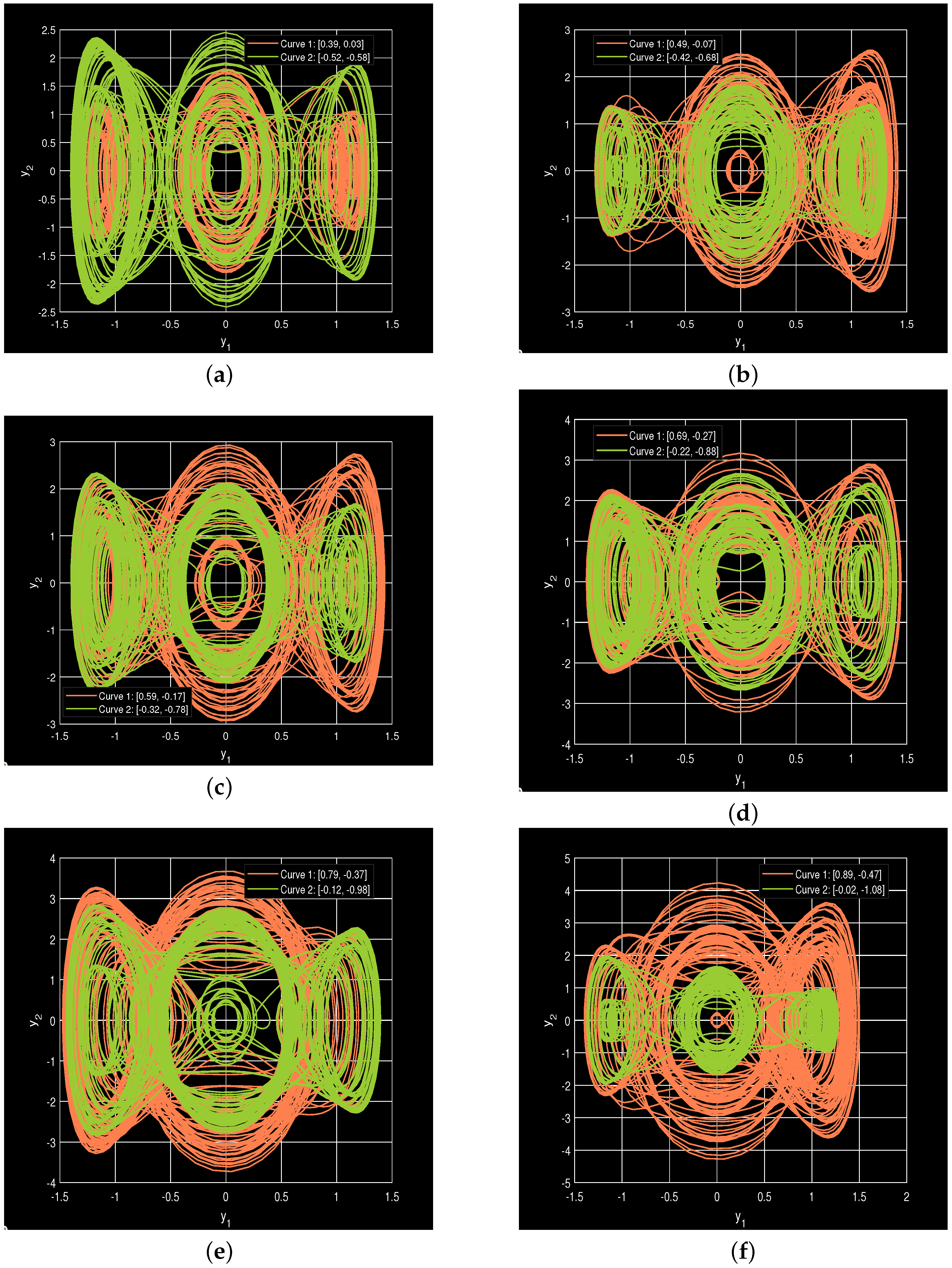
Figure 6. Coexistence of chaotic attractors demonstrating multi-stability. (a) Comparison of chaotic and periodic behavior from distinct initial conditions. (b) Coexistence of periodic and chaotic behaviors on a single trajectory, showing rapid switching between orderly and disorderly regions. (c) A constrained trajectory versus one with large variations, showing how small displacements lead to different attractor basins. (d) With ω = 0.4 , two distinct chaotic attractors are shown: one wide and folded, the other developing from periodic motion. (e) At ω = 0.5 , both trajectories are fully disordered; one (coral) covers a larger space while the other (olive) shows nested, trapped regions. (f) At ω = 0.6 , a fully developed, wide-ranging chaotic attractor coexists with a compact, localized attractor.
Algorithms 18 00681 g006

3.4.2. Analysis Based on Figure 7

  • Figure 7a: The dynamical responses exhibit multi-stability when parameters are changed to have the value of ω = 0.2 . The magenta curve (Curve 1), with the initial condition of [0.39, 0.03], looks like a broad, erratic-looking object. The yellow curve (Curve 2) that originates at [−0.52, −0.58] is extremely localized, consisting of a tight, dense attractor. This dramatic difference in geometry depicts how sensitive the system is to initial conditions.
  • Figure 7b: With slightly perturbed initial conditions of [0.49, −0.07] for Curve 1 and [−0.42, −0.68] for Curve 2, the trajectories evolve into attractors which overlap partly. Curve 1 is tilted more to the left side of the phase space, with Curve 2 having a concentration of loops that are spread out better to the right. Such trajectories emphasize the important role of even tiny variations in initial conditions, as the effect is asymmetric.
  • Figure 7c: The points begin from (0.59, −0.17) and (−0.32, −0.78), and the trend is the same. The numerous attractors indicate that the system is in a constant state of changing between ordered and chaotic based on the initial state of the system. This can be much like the classical chaotic systems, where the slightest change in factors can cause a system to shift to an alternate attractor type.
  • Figure 7d: By changing the initial point to (0.69, −0.27) and (−0.22, −0.88), the attractors are more densely represented with multiple points of loop cross-over. The two trajectories remain in the fixed regions, but because they have different shapes, they indicate a transition between one stability regime to another. Its crowded loops indicate that the system is probably alternating between quasi-periodic and weakly chaotic dynamics and has coexisting attractors.
  • Figure 7e: The orbits, i.e., those with starting point (0.79, −0.37) and (−0.12, −0.98), appear to be less organized in the phase space. The magenta group has most of the loops on the left and the yellow group stretches more on the right. This means that even a slight alteration in the initial position may result in a quite different development of systems.
  • Figure 7f: This depicts the vector fields of conditions ( y 1 , y 2 ) = ( 0.49 , 0.07 ) and ( y 1 , y 2 ) = ( 0.42 , 0.68 ) . The system described after the magenta trajectory is more predictable, whereas the one described by the yellow trajectory is less predictable. This implies that a system may move in almost a repetitive manner or be disorganized depending on the point of beginning. What is indicated by the overlapping and non-overlapping loops is that the system is able to exhibit various behaviors at the same time, which is a characteristic feature of multi-stability.
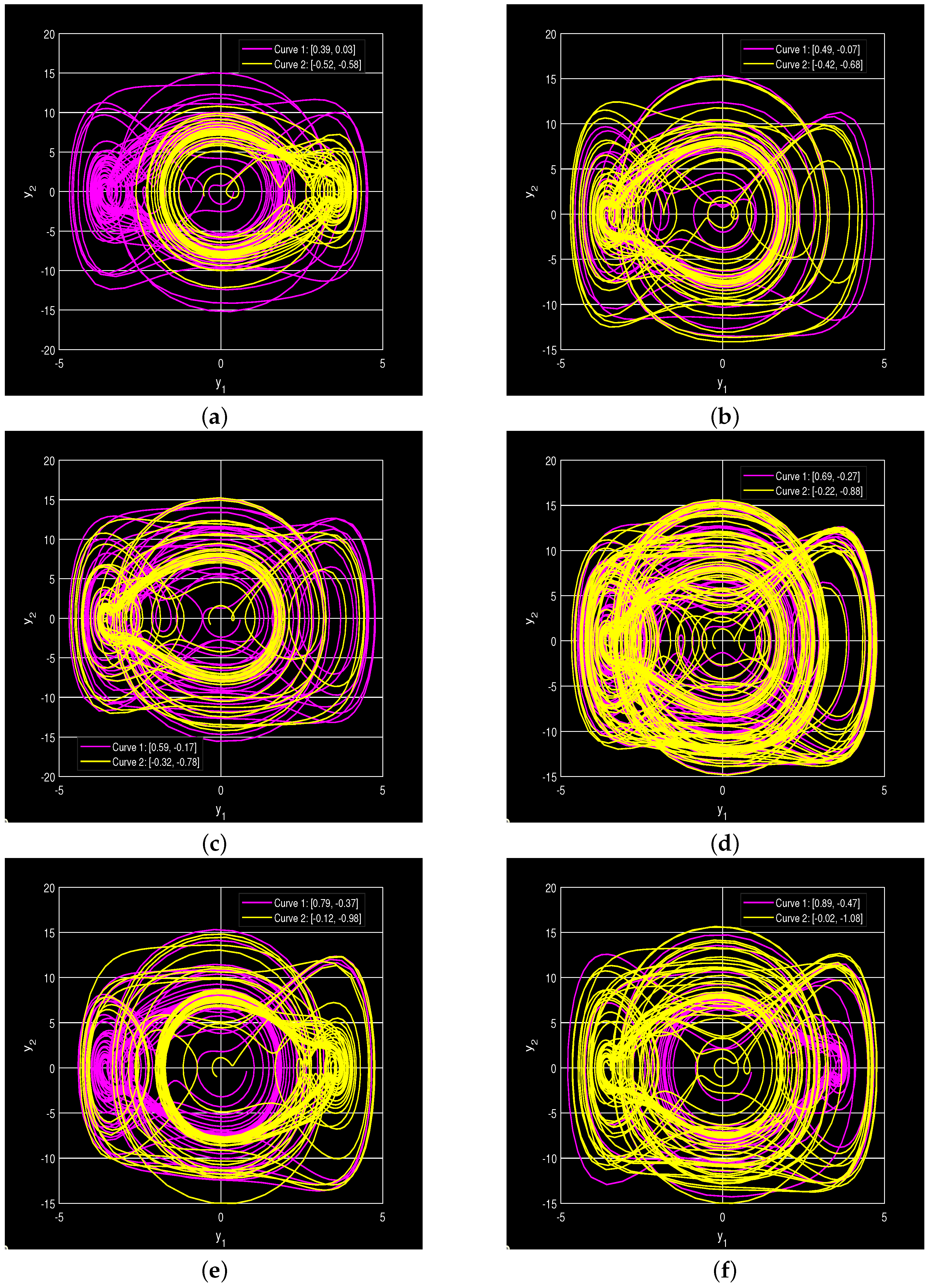
Figure 7. Multiple coexisting attractors under a new parameter regime. (a) With ω = 0.2 , a broad, erratic attractor (magenta) coexists with a localized, dense one (yellow). (b) Partly overlapping attractors showing asymmetric spatial distribution (magenta left, yellow right). (c) Coexisting attractors confirm the system’s state (ordered or chaotic) is highly dependent on initial conditions. (d) Denser attractors with more cross-overs suggest a transition between quasi-periodic and weakly chaotic regimes. (e) Disorganized orbits show clear spatial separation, with magenta loops on the left and yellow on the right. (f) A more predictable trajectory (magenta) coexists with a less predictable, disorganized one (yellow).
Algorithms 18 00681 g007
The nonlinearity of the system is emphasized by this resilience, and the system has a strong response to initial conditions. It is highlighted that the starting situation is prone to small changes, which in turn will lead the complex or chaotic system to behave in very different ways.
Algorithm 1: Multi-stability Analysis
Algorithms 18 00681 i001

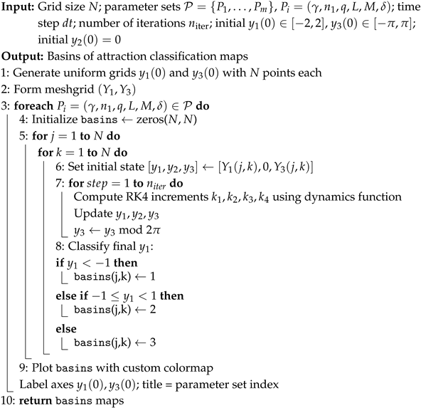
3.5. Basin Analysis

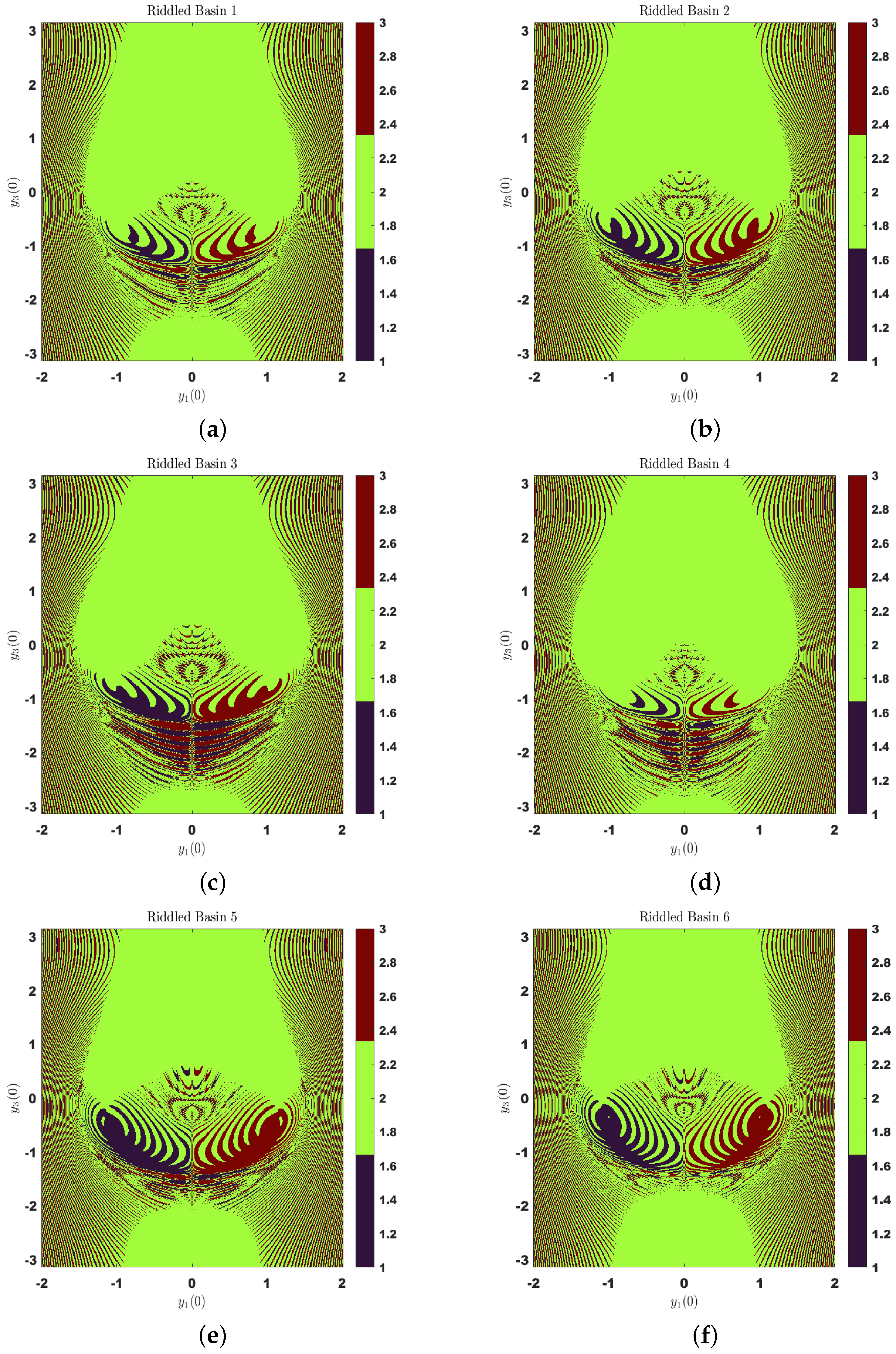
  • Analysis of Figure 8a: As shown in Figure 8a, a basin with riddled topology means that the attractor regions are closely intertwined. Slight variations in the initial values y 1 ( 0 ) and y 3 ( 0 ) can cause the trajectory to look very different, even with everything else fixed. Six alternating colored regions illustrate a riddled basin structure, where results are strongly influenced by starting conditions and can be quite unpredictable. Looking around the central and lower parts of the plot, the lines between the basins have a detailed and fractal pattern, indicating that the system includes chaotic behavior. Such actions align with systems that are influenced by both strong nonlinearity and periodic changes in the environment.
  • Analysis of Figure 8b: A slight variation in the initial conditions (keeping y 2 ( 0 ) unchanged) results in a riddled basin that looks markedly different. Although the global structure still has a stable core, the domain boundaries can move and realign, demonstrating how sensitive the landscape is to tiny fluctuations. This restarts, showing that the limits of the basins are not perfect and revealing that the system stays unpredictable, even when practically the same conditions are used at the start. Chaotic behavior like this appears near important bifurcation points in systems.
  • Analysis of Figure 8c: In Figure 8c, the basins appear more broken and less continuous than in the other two figures. A slight change in the initial value of y 2 produces attractor figures that are spread out and less uniform. Since the phase space is less cohesive and the colors are arranged randomly, it appears that the system could be close to a chaotic region. The change from a riddled to a scattered basin shows that complexity is higher in the system and that accurate starting conditions are required to avoid uncertainty as time goes on.
  • Analysis of Figure 8d: Figure 8d displays a deeply disordered and defective riddled basin landscape. The system has no chance to adjust its fixed parameters or the value of y 2 ( 0 ) , yet changing y 1 ( 0 ) and y 3 ( 0 ) by small amounts results in very different perspectives in the long run. When different colors are seen together within the pattern, it indicates that there are numerous beautiful attractors close together, but the lack of long, continuous colors shows how sensitive to chaos the system can be.
  • Analysis of Figure 8e: Figure 8e shows what a basin structure looks like, featuring regions that are only partially coherent. There are slightly more continuous colored regions in the attractor domains than in Figure 8d, hinting at a small change toward areas with local stability. When q increases to 11.0 and d decreases to 0.05, the fractal lines of the basins shift and make some regions more prominent than others. However, the system multi-stability and sensitivity to starting conditions are still present due to its complex filaments and collapsed neighborhoods.
  • Analysis of Figure 8f: The pattern in Figure 8f is still riddled, but with much simpler attractor regions than before. The system nonlinearity and slow rate of modulation make it possible for some basins to spread and become dominant in some regions of the initial condition space. But little traces of chaotic filigree and bands of color can still be seen in the phase plot during this phase. There is evidence of a regulating regime that is not yet fully stable, since some of its elements remain truly chaotic.
    Together, Figure 8a–c make it clear that a modest difference in y 2 ( 0 ) results in major changes in the way attractor patterns form. It makes clear that the system is very sensitive to its conditions and tends to have unpredictable long-term behavior. Figure 8d–f add further details on how parameters such as nonlinearity depth, external force strength, and frequency range make a difference. The computational method used to generate these basins is detailed in Algorithm 2, and the specific parameters are summarized in Table 4. The set of frames explains how nonlinear systems that see a repeating external force often display dynamic behavior and are very responsive. Such basin areas, full of intricately jumbled areas of similar attractors, show that the system is multi-stable and chaotic. They show that some basins have turned from being enclosed by chaos to being separated by structures, showing signs of stability that replace instability. The presence of chaotic multi-stability and major sensitivity can still be noted, as these figures retain the essential features of riddled or fragmented basins, despite the transitions.
Algorithm 2: Scattered Basin Classification via RK4 Integration
Algorithms 18 00681 i002

4. Attractor Geometry and Phase Space

4.1. Phase Portraits

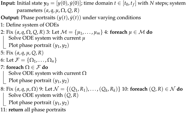
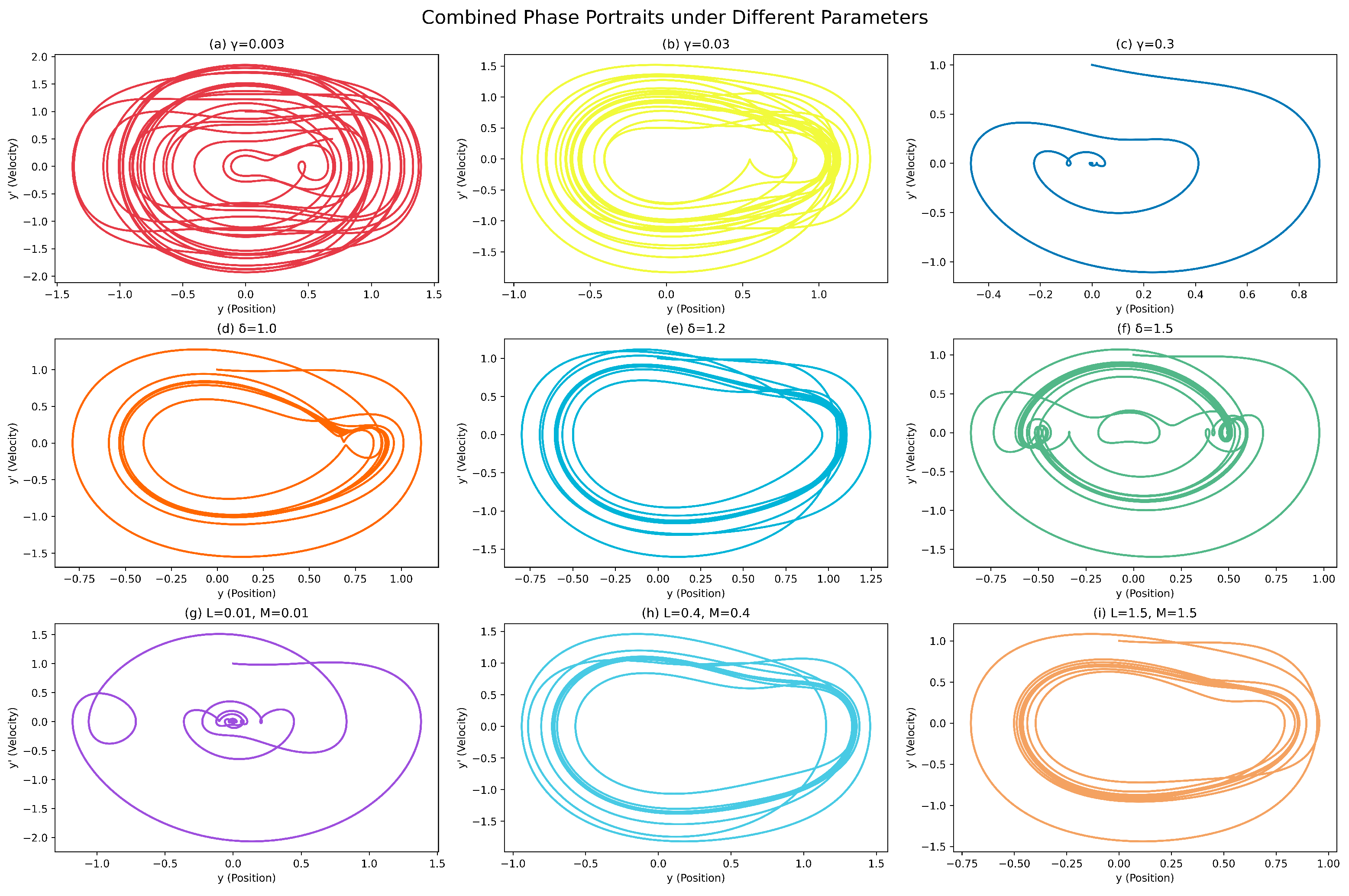
The analysis of each phase plot is performed using nonlinear dynamics theory. The various cases in Figure 9 show the motion of a particle at varying rates of damping and magnitudes of the nonlinear terms. The computational method used to generate these portraits is detailed in Algorithm 3, and the full set of parameters for each case is summarized in Table 5.

4.1.1. Effect of Varying Damping Coefficient ( γ )

The change in the damping coefficient affects the way the movement traces are shown in Figure 9a–c.
  • Low damping ( γ = 0.003 ): When there is a little energy added, small oscillations continue for a relatively long period. The orbits are very broad and curved, which reveals a sluggish reduction in their energy. For this regime, the phase portrait has the potential to demonstrate periodic or chaotic behavior, mainly due to strong nonlinear and forcing effects.
  • Moderate damping ( γ = 0.03 ): As γ becomes 0.03, the system works more efficiently to damp complicated modes. The spirals surround each other more closely as the changes converge on a stable-state point. Such a design is nearly at critical damping, helping to avoid overshoot while still permitting damped oscillations.
  • High damping ( γ = 0.3 ): If γ equals 0.3 or greater, the system becomes damaged and is dominated by linear dissipative forces rather than by restoration and nonlinear forces. All paths fast approach the origin with very few oscillations. There is no need for complex motions and complex attractors cannot develop. This shows that damping is an option to reduce nonlinear or chaotic motions.

4.1.2. Effect of Varying Natural Frequency ( δ )

In the next three cases, Figure 9d–f, the natural frequency is used to govern the oscillatory response of the system.
  • Resonant frequency ( δ = 1.0 ): If δ is close to one and especially close to the excitation frequency, the system becomes susceptible to resonance from the parametric drive. Under this condition, the closed-loop motion seen in the phase space is only possible for Mathieu-type systems at δ = 1.0 . In this regime, the motion often repeats itself periodically or almost periodically.
  • Increased frequency ( δ = 1.2 ): With δ at 1.2, the structure of the phase space becomes more complicated. The presence of loops and unusual swings in paths means that the system is performing nonlinear resonance. The phenomenon of internal resonances or frequency locking is responsible for joining different modes of vibration together. It is also possible that, under the right conditions, this step marks the start of chaotic behavior through quasiperiodicity.
  • High frequency ( δ = 1.5 ): When δ = 1.5 , the phase portrait exhibits a densely populated structure, with trajectories no longer forming closed orbits, but instead densely filling extended regions of the phase space. This behavior is indicative of the onset of chaos in the system. Such a transition is characteristic of parametric resonance, wherein the frequency modulation couples with the system natural frequency in a manner that destabilizes its dynamics.

4.1.3. Effect of Varying Nonlinear Coefficients (L and M)

The amplitude-dependent restoring forces result from the nonlinear terms L y 1 3 and M y 1 5 that cause the system to show a harmonic movement, but not at an even pace, as illustrated in Figure 9g–i.
  • Weak nonlinearity ( L = M = 0.01 ): For very small values, there is only a small nonlinear effect, so the system converges to its equilibrium point smoothly. The phase portrait consists of symmetric spirals that look much like those of a damped harmonic oscillator.
  • Moderate nonlinearity ( L = M = 0.4 ): The impact of the coefficients can be seen more clearly at 0.4. The plots reveal that the motions follow looping paths with different thickness and shape, demonstrating the influence of nonlinear stiffening or softening. Sinusoidal motion is interrupted, and the frequency depends on the system amplitude, which is a sign of Duffing-like systems. Nonlinearity in the system starts to change the energy landscape, offering chances for multiple stable states.
  • Strong nonlinearity ( L = M = 1.5 ): With high state values, the nonlinear behaviors become the main factor in the dynamics. The density increases, and the way the phase space is folded supports the idea of chaotic attractors. Here, more than one attractor may exist, so the long-term actions of the system are closely linked to where it starts from. This type of regime shows the effects of riddled basins of attraction, bifurcations, and global instability.
When nonlinear stiffness, damping, and parametric forcing interact, the system forms a powerful structure that cannot be explained by simple linear mathematics. Systems develop their phase-space structure mainly because of each chosen parameter. The conservation of energy, the interaction of vibration with its frequency, and the complexity in the solution space depend on damping, natural frequency, and nonlinearities. Whether limit cycles, chaos, bifurcations, or fixed points are formed depends on the settings of the values.
Table 5. Combined effects of damping ( γ ), frequency ( δ ), and nonlinearity ( L , M ) on observed system dynamics.
Parameter (Symbol)ValueObserved DynamicsInterpretation
Damping ( γ )0.003Large spiral orbits, transient loopsWeak damping allows complex trajectories and longer energy retention
0.03Moderate convergence, reduced loopsIntermediate damping suppresses large excursions
0.3Rapid convergence to originStrong damping dominates; motion decays quickly
Frequency ( δ )1.0Regular loops, symmetric trajectoriesResonance with excitation; periodic or quasi-periodic motion
1.2Deformed loops, twisting phase pathsNonlinear resonance; possible mode-mixing
1.5Dense and irregular patternsParametric resonance; onset of chaos likely
Nonlinearity ( L , M )0.01Smooth convergence, near-linearSystem behaves almost linearly
0.4Deformed loops, amplitude-modulated pathsNonlinearities influence amplitude-frequency relations
1.5Dense, chaotic-looking phase spaceStrong nonlinear effects dominate, complex or chaotic motion
Algorithm 3: Phase Portraits of Nonlinear ODE System
Algorithms 18 00681 i003

4.2. Chaotic Attractor

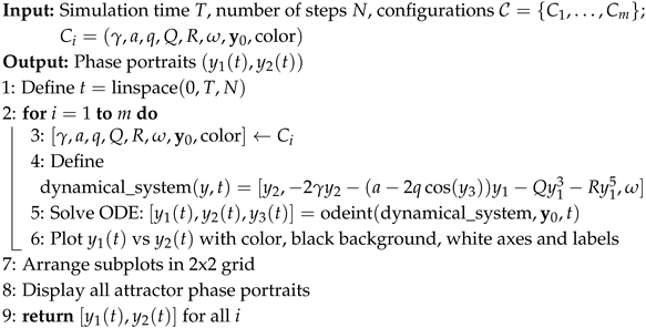
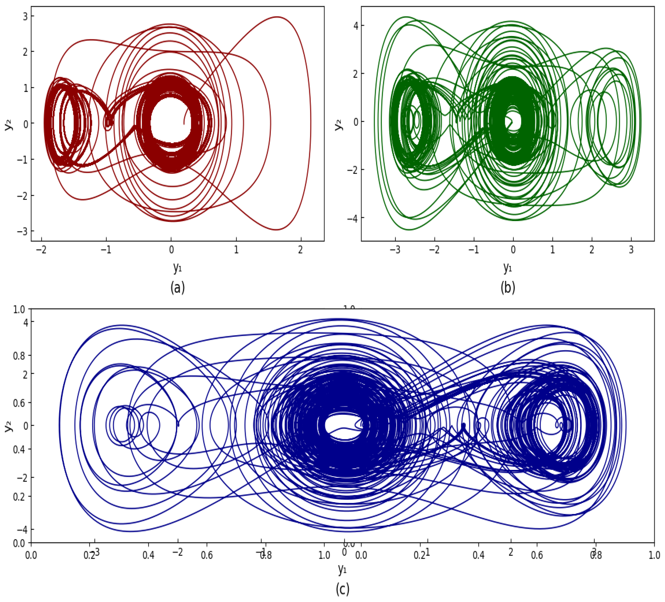
The presence of distinct attractors in chaotic systems is due to their high sensitivity to small changes in parameters and initial conditions. In this study, a system with quintic nonlinearity, damping, and external inputs is examined. The effects of altering parameters and starting conditions on the attractors are investigated in three different cases. The computational procedure used for this investigation is presented in Algorithm 4.
In the first two cases, shown in Figure 10a,b, the same initial conditions are applied with different system settings to understand how nonlinear and external factors affect the dynamics. In the third case, shown in Figure 10c, the initial conditions are updated while using the same parameters as in the second case, showing the multi-stability of the system.

4.2.1. Analysis of Figure 10a

Observed dynamics: We studied the system where quintic nonlinearity is the major determinant of stabilizing chaos motions, and it was set up with the following parameters: γ = 0.038 , n 1 = 2.05 , q = 4.01 , L = 0.08 , M = 0.65 , and δ = 0.2 . Considering the initial conditions, y 0 = [ 0.2 , 0.03 , 0.25 ] , at these settings one obtains a small and slightly chaotic area of the phase space. The high quintic nonlinearity ( M = 0.65 ) massively suppresses the large fluctuations and demonstrates the fact that the phase-space paths are not very divergent. The attractor can also be found well contained even with external forcing, which shows that the contribution of the nonlinear effects is appropriate in balancing the effects of the forced variables. As a result of the rather low damping coefficient ( γ = 0.038 ), the system will still oscillate, although the oscillations will not be too sporadic. The chaotic attractor that emerges is smooth and thick, which brings out the significance of the quintic stiffness in providing a consistent variety of variations.

4.2.2. Analysis of Figure 10b

Observed dynamics: The system phase-space structure experiences a strong change with new nonlinear parameter values fixed to the following: γ = 0.048 , n 1 = 2.75 , q = 4.1 , M = 0.065 , and δ = 0.22 . A stronger cubic nonlinearity of the system, parameter ( L = 0.28 ), is used to reconfigure the dynamics of the initially chosen attractor state y 0 = [ 0.2 , 0.03 , 0.25 ] ; the dynamics are reshaped by a dominant cubic nonlinearity ( L = 0.28 ), giving rise to a larger and more disordered chaotic geometry. This is in contrast with a much less pronounced quintic nonlinearity ( M = 0.065 ), which does less to stabilize and lets chaos do more to disperse. Even with high damping (i.e., high value of the damping coefficient, given as γ = 0.048 ), the cubic term is very large and contributes considerably to high dynamical complexity. Additionally, augmented external forcing amplitude ( q = 4.1 ) and frequency ( δ = 0.22 ) bring about faster oscillations in time, increasing the chaotic response. The attractor that results is more dominated by broader loops and longer trajectories, demonstrating the amplification of the chaotic nature of the system by further cubic nonlinearity.

4.2.3. Analysis of Figure 10c

Observed dynamics: The major characteristic of the system is the multi-stability which presents a particular chaotic attractor, appearing only after the change in the initial conditions and the system parameters remaining the same as in the preceding scenario. With the initial condition of the system being y 0 = [ 0.02 , 0.06 , 0.05 ] , the system is drawn to an entirely new chaos. This behavior shows that there are various basins of attraction which contain the long-term trajectory of the systems by different attractors based on the initial point of the system. Even though the resulting dynamics are chaotic, this new attractor has different properties than the one noticed before, and this proves the fact that the state of the system with time is extremely dependent on its initial conditions.
This result demonstrates that parameters and alterations in initial conditions are very influential to the way the system evolves. It implies that the same system parameters can in some cases give rise to different long-term models, which demonstrates that minor alterations in initial conditions of chaotic systems can have a strong influence on the end attractor. The fact that there are various attractors which can be used means that when employing such systems, control becomes precise, because a minor change can lead to a significant change in the performance of the system.
Algorithm 4: Attractor Visualization via High-Resolution ODE Integration
Algorithms 18 00681 i004

4.3. Return Map

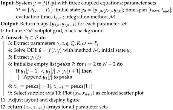
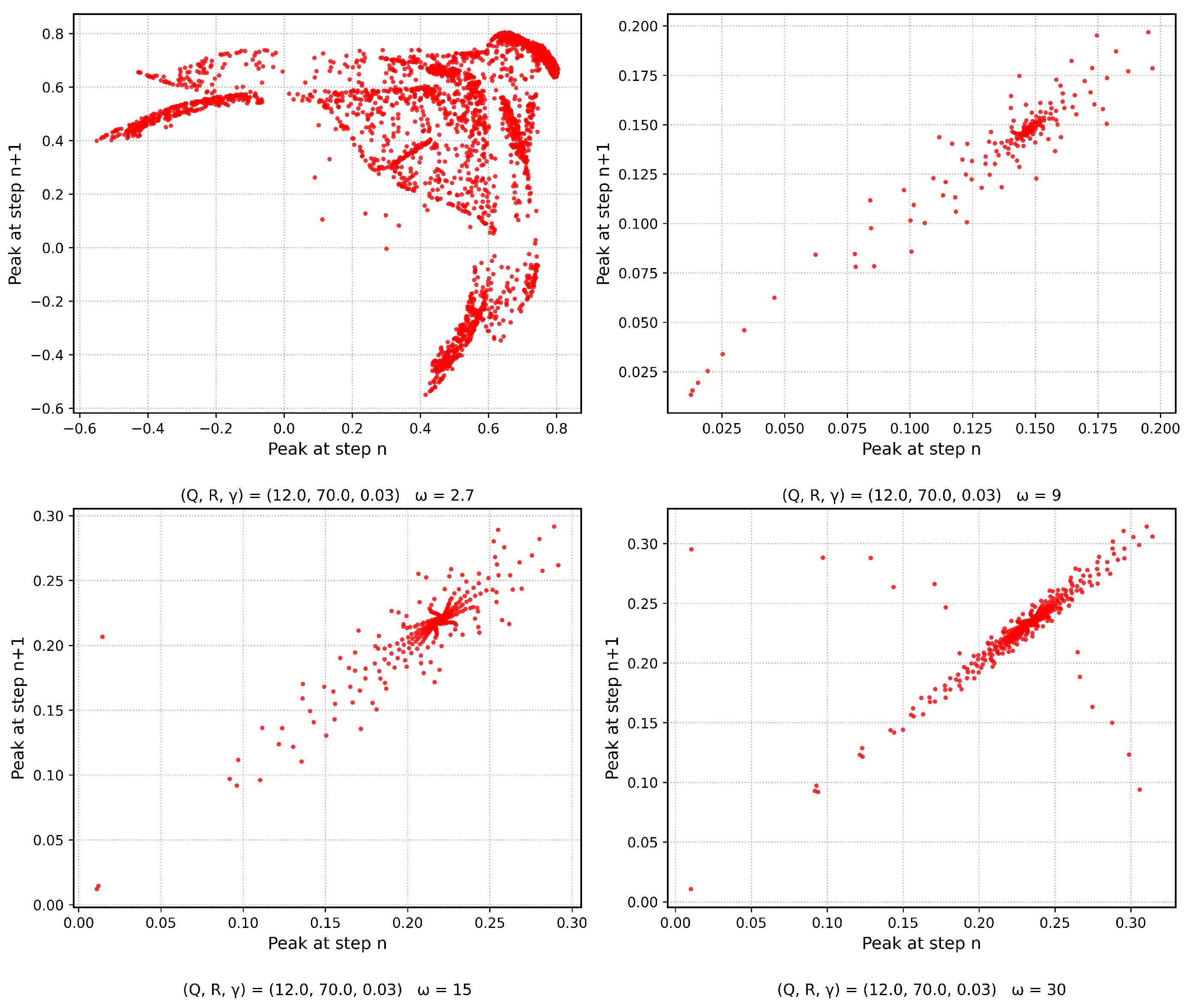
For the dynamical system in Figure 11, a return map analysis reveals how the system motion changes as the parameter δ is varied. The sequences of peaks in y 1 serve as the core pattern for each map to present the movements of the system. The computational procedure is detailed in Algorithm 5.

Analysis of System Motion by Varying Frequency ( δ )

Chaotic motion ( δ = 2.7 ): For δ = 2.7 , the return map shows segments that are scattered in many directions, implying that the system is chaotic. The order of points is difficult to forecast, since the slight variation in initial values leads to a major variation with time, an indicator of deterministic chaos. This action encompasses bizarre lures that make the system shift to unforeseen locations among diverse conditions instead of stabilizing itself in routine patterns.
Transition to structured motion ( δ = 9 ): With a further increase in the parameter ( δ ) to 9, the return map itself is more familiar, as small pieces tumble out of the chaos to a more organized structure. The reduction in the number of scatter points means that the system is transitioning to different forms of motion to near-periodic or low-dimensional chaotic flow.
Intermittent behavior ( δ = 15 ) : At the point of the return map that is at the value of at least 15, we can see the circles crowded with sparse points. This shows that there is a periodic behavior in which the system switches between the chaos and order which is typical of the intermittent behavior. The system lies between stability and chaos, whereby there are order and disorder components, which emerge as a result of interacting forces.
Emergence of stability ( δ = 30 ): When the value of the parameter, which is the delta, becomes equal to 30, the formations which the return map offers demonstrate that the system is about to enter common oscillations. These trends indicate that the system has attained stability as a result of external forces guiding the movements and not the creation of stochastic outcomes.
When you add more and more to the value of delta, the system is brought to a more faithful rotation and is therefore made to be responsive to external forces. According to the results of the simulation, an increase in the value of the parameter of uncertainty, denoted by the value of delta, will result in reduced chaos and cause the system to act in a specific manner. When it is subjected to external frequencies based on standard nonlinear principles on the vibrating systems, the latter sets out in a systematic motion. The applications of these findings are useful in a number of applications such as automated systems, biological signaling, and electronic systems.
Algorithm 5: Return Maps for a Dynamical System
Algorithms 18 00681 i005

5. Spectral and Temporal Properties

5.1. Power Spectrum

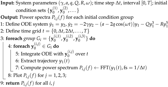
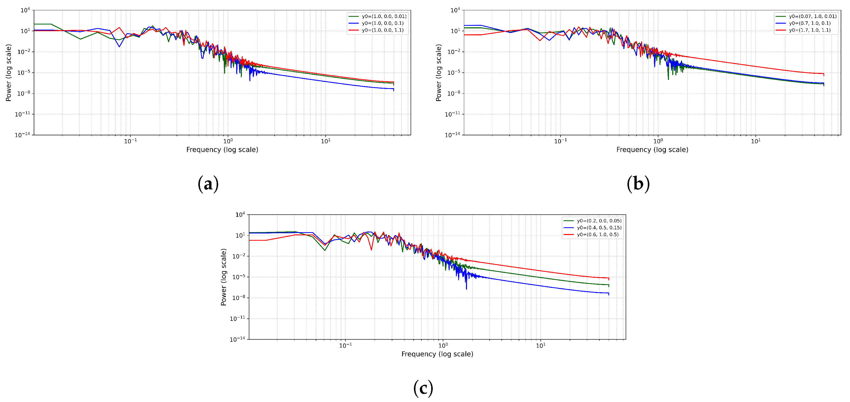
The frequency-based analysis of the power distribution is shown to the system under analysis in different starting conditions. This analysis is performed using the computational method presented in Algorithm 6. The power spectrum plot is plotted on a logarithmic scale, where the frequency is plotted on the horizontal axis, and the magnitude of the power is plotted on the vertical axis. The analysis shows the most significant frequency components, their behavior under the influence of system variations, and the way they may be influenced by various types of movement. For chaotic dynamics, the power spectrum typically spans a wide range of frequencies, producing a broad and continuous profile that reflects the system’s irregular, aperiodic behavior. In contrast, periodic motion manifests as sharp, well-defined peaks at specific frequencies, corresponding to the regular repetition of the underlying oscillations.
  • Spectral analysis of Figure 12a: Spectral analysis was applied to three different initial conditions: ( y 1 , y 2 , y 3 ) = ( 1.0 , 0.0 , 0.01 ) , ( 1.0 , 0.0 , 0.1 ) , and ( 1.0 , 0.0 , 1.1 ) . At low frequencies ( f < 10 1 ), the three spectra have large power amplitudes which tend to decrease with frequency. The power levels at the intermediate range ( 10 1 f 10 0 ), show much more distinct values, with the yellow spectrum containing a more powerful magnitude of power than the magenta and cyan spectra, meaning more mid range frequencies contribute to the spectrum. Beyond ( f > 10 1 ) frequencies, all spectra show a decreasing pattern with slight amplitude fluctuations, which are high frequency modes dampened. This general spectral activity highlights the sensitivity of the system’s frequency response to its initial conditions, especially at mid and high frequency regimes.
  • Spectral analysis of Figure 12b: The analysis has again been performed under a distinct choice of initial conditions: ( y 1 , y 2 , y 3 ) = ( 0.07 , 1.0 , 0.01 ) , ( 0.7 , 1.0 , 0.1 ) , and ( 1.7 , 1.0 , 1.1 ) . As previously noted, the size of the power also decreases with increasing frequency. Nevertheless, in the mid frequency range, the yellow curve exhibits more pronounced oscillatory features, indicating that variations in initial conditions can influence the distribution of energy across different frequency bands. At a high frequency, all curves have a decay pattern which is the same but with slight variations, representing some differences in the system’s high frequency dynamics. These mid range oscillations indicate the existence of some underlying quasi-periodic structures in the primary chaotic attractor.
  • Spectral analysis of Figure 12c: This analysis indicates the power distribution of initial conditions ( y 1 , y 2 , y 3 ) = ( 0.2 , 0.0 , 0.05 ) , ( 0.4 , 0.5 , 0.15 ) , and ( 0.6 , 1.0 , 0.5 ) . The resultant spectra act in a similar way as the earlier cases, except that the power amplitudes are higher at lower frequencies and tend to diminish at higher frequencies. There is, however, a very clear distinction in the mid range of frequencies, wherein the cyan curve is much lower than the magenta and yellow curve. The other two curves have long-term oscillations, but the yellow curve always has a minor advantage in power. This confirms that not only the direction in the phase space but also the energy distribution over frequencies is extremely sensitive to the starting point of a system, which is a prominent multi-stability property.
It seems that initial conditions are significant determinants of the distribution of power between the frequency bands. The less energy the system initially has, the more it will concentrate on lower frequencies, but as the energy increases, the oscillations will be more pronounced at the middle to high frequencies of the spectrum. These differences in spectral measurements also suggest the notion that the behavior of the system depends on the initial condition of the system, which highlights the great influence of nonlinearity.
Algorithm 6: Power Spectrum Analysis of Nonlinear ODE System
Algorithms 18 00681 i006

5.2. Recurrence Plots

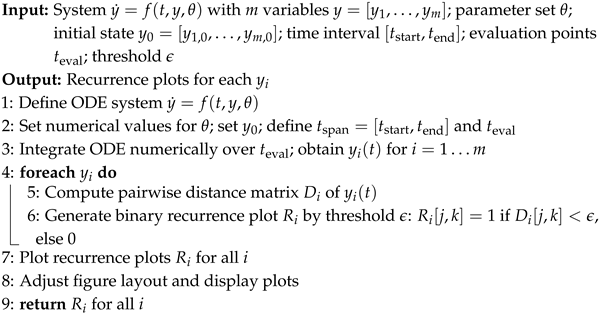
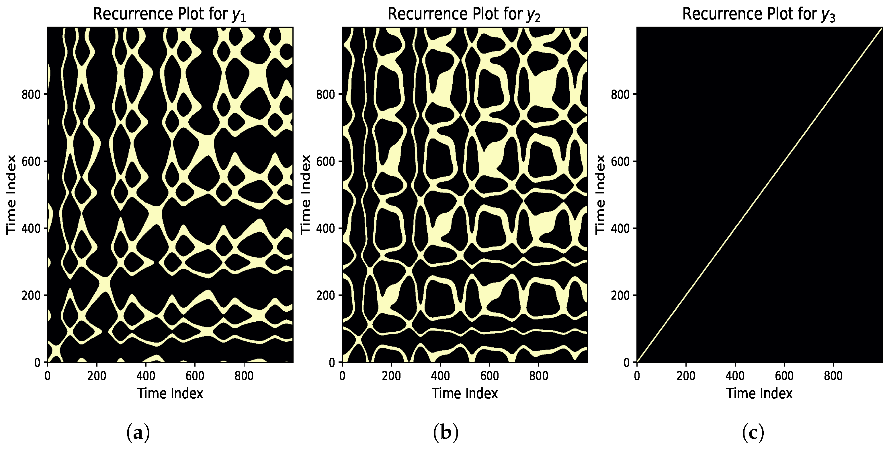
Recurrence plots (RP) are an easy way of visualizing the frequency of occurrence of states within a dynamic system; thus, they are a handy time-series analysis tool. The algorithm used to generate the RPs for this study is detailed in Algorithm 7. An RP reveals the where and how of returning to the same behaviors of a system, hence displaying new periodic structures and irregularities. The manner in which an RP is presented provides the details about the nature of the information; the presence of extensive and prevalent diagonal lines is an indicator of periodicity, and the presence of sporadic short lines depicts that the data are not regular. White or sparse regions represent the times when states change, whether they are noisy, or whether there is an irregular change. The horizontal and vertical lines are also the states of laminar flow that are common in turbulence and phase transitions. Essentially, the plot guides a complicated time series into a graphical texture, which discloses the dynamical regime of that time series.
  • Analysis of Figure 13a: The pattern observed in the recurrence plot of y 1 is not regular and contains interrupted diagonal lines and numerous intricate designs. This implies a complexly behaving system that is very sensitive to the initial conditions. The pattern is not repeated in each and every period due to the lack of long diagonal structures. The texture of the plots resembles a mature chaotic regime. Rather, the changes seem to be influenced by peculiar interactions, and the evolution seems less predictable.
  • Analysis of Figure 13b: Unlike the plot of y 1 , the plot of y 2 has more noticeable patterns and has both diagonal lines and areas enclosed by vertical lines. Thus, there is certain basic periodicity, but the system is influenced by irregular and diffuse outliers. The fact that the recurrences are in a grid formation shows that the system may display quasi-periodicity. This indicates a motion that is more ordered than pure chaos but not perfectly periodic. Frequently, such behavior happens when a system displays weak chaos or if there are interactions.
  • Analysis of Figure 13c: The recurrence plot in Figure 13c shows y 3 behaving in a way that is different from the others, forming just one long diagonal line. As a result, the motion is fully periodic, with the system repeating the same path over and over. Because scattered recurrence points are missing, the system appears to be stable and without noticeable changes or chaos. This represents the simple, periodic drive of the system.
All of the results highlight a major shift in the behavior of the system along its key variables. The third sub-system, y 3 , follows a repeating periodic pattern; the second subsystem, y 2 , contains quasiperiodic features; and the first system, y 1 , displays chaotic movement. The preceding view explains how the system goes from simple to complex and becomes more sensitive to details from the start. Because there is chaos in one coordinate and quasi-periodicity in the other, nonlinear effects are influencing the system, which could result in transitions or bifurcations. Knowing about these recurrence structures makes it simpler to recognize the factors that play a role in the system’s activities.
Algorithm 7: Recurrence Plots for a 3D Dynamical System
Algorithms 18 00681 i007

6. Conclusions

In this paper, we thoroughly examined the multi-faceted dynamics of the DM-CQDO and came up with a number of important scientific findings. The first, the detailed stability diagram of the system, mapping the large-scale structure of the chaotic and periodic regimes of the system, is our main observation. Moreover, we found the period-doubling cascade as the primary approach to chaos and quantitatively studied how damping of a system regulates the stability thresholds. We also defined pervasive multi-stability of the system via Lyapunov analysis and by image representation of the fractal character of attractor basins of the system. This was only possible through an integrated workflow, combining data-driven model discovery with SINDy with various classical dynamical systems analyses, which showcases an effective method of exploring complex systems in which the equations of motion are not necessarily known. Such a combination of methods fills in an important literature gap by offering a feasible methodology where numerous studies use a small pool of tools. One of the strengths of the given framework is that it has very wide applications, because the analysis uses solely the trajectory data as the input; thus, the same pipeline can be used for a large variety of nonlinear systems in various applications in mechanics, electronics, optics, and biology. The work is therefore a paradigm in the coming data-driven studies of complicated dynamics.
As much as the proposed framework has shown good performance, the limitations of the proposed framework must be noted as well as the potential areas into which the research can be advanced in the future. The accuracy of the SINDy-based discovery depends on the quality of time-series data and may be affected by measurement noise or sparsely sampled trajectories. Moreover, it can be optimized further in cases when it should be extended to high-dimensional systems. Nonetheless, the modularity of the pipeline is an encouraging base of studies to come, especially the use of the pipeline on experimental data and stochastic perturbation to investigate its stability when subjected to real world uncertainties. These challenges mark the next stage of advancement for data-driven approaches in the study of nonlinear dynamical systems.
Based on this structure, future studies can take a number of promising computational directions:
  • Future efforts could focus on developing computationally efficient, high-resolution algorithms capable of resolving the intricate fractal structure of basin boundaries in nonlinear dynamical systems.
  • Future efforts could ystematically monitor the development of attractors to automatically identify complex global bifurcations by using parameter continuation algorithms.
  • Designing and testing parametric control or delayed feedback algorithms can help manage or suppress the chaotic behavior identified by our framework.
  • Enhancing the analysis pipeline with machine learning algorithms can be used to automatically classify different dynamic regimes in real time.
In summary, this paper provides more than a detailed characterization of a specific oscillator; it offers a valuable algorithmic methodology for the sophisticated analysis of chaotic phenomena across a diverse range of parametrically driven nonlinear systems in science and engineering.

Author Contributions

Conceptualization, A.J.; methodology, A.J.; software, B.I.; validation, A.J. and M.M.; formal analysis, B.I.; investigation, B.I. and M.M.; writing—original draft preparation, B.I.; writing—review and editing, M.M. and A.J.; visualization, A.J. and M.M.; supervision, A.J. and M.M.; project administration, A.J.; financial acquisition, A.J. All authors have read and agreed to the published version of the manuscript.

Funding

This article has been produced with the financial support of the European Union under the REFRESH—Research Excellence For Region Sustainability and High-tech Industries, project number CZ.10.03.01/00/22_003/0000048 via the Operational Programme Just Transition.

Data Availability Statement

The article contains all of the data that were analyzed for the current project.

Conflicts of Interest

The authors declare that they have no conflicts of interest to report regarding the present study.

Abbreviations

The following abbreviations are used in this manuscript:
SINDySparse Identification of Nonlinear Dynamics
DM-CQDODamped Mathieu Cubic–Quintic Duffing Oscillator
MEMSMicro-Electro-Mechanical System
NEMSNano-Electro-Mechanical System
PINNsPhysics-Informed Neural Networks
STLSQSequentially Thresholded Least-Squares
RK4Fourth-Order Runge–Kutta
RPRecurrence Plot

References

  1. Scanlan, R.H.; Tomko, J.J. Airfoil and bridge deck flutter derivatives. J. Eng. Mech. Div. 1971, 97, 1717–1737. [Google Scholar] [CrossRef]
  2. Franco, H. Wavelet analysis of a nonlinear oscillator transient during synchronization. Int. J. Bifurcat. Chaos 1996, 6, 2557–2570. [Google Scholar] [CrossRef]
  3. Matsumoto, T. A chaotic attractor from Chua’s circuit. IEEE Trans. Circuits Syst. 2003, 31, 1055–1058. [Google Scholar] [CrossRef]
  4. Kovacic, I. On the motion of a generalized van der Pol oscillator. Commun. Nonlinear Sci. Numer. Simul. 2011, 16, 1640–1649. [Google Scholar] [CrossRef]
  5. Glass, L.; Mackey, M.C. From Clocks to Chaos: The Rhythms of Life; Princeton University Press: Princeton, NJ, USA, 1988. [Google Scholar]
  6. Slotine, J.J.E.; Li, W. Applied Nonlinear Control; Prentice Hall: Englewood Cliffs, NJ, USA, 1991. [Google Scholar]
  7. Nayfeh, A.H.; Balachandran, B. Applied Nonlinear Dynamics; Wiley: New York, NY, USA, 1995. [Google Scholar]
  8. Nayfeh, A.H.; Mook, D.T. Nonlinear Oscillations; John Wiley & Sons: New York, NY, USA, 2024. [Google Scholar]
  9. Lai, S.K.; Lim, C.W.; Wu, B.S.; Wang, C.; Zeng, Q.C.; He, X.F. Newton-harmonic balancing approach for accurate solutions to nonlinear cubic-quintic Duffing oscillators. Appl. Math. Model. 2008, 33, 852–866. [Google Scholar] [CrossRef]
  10. Kovacic, I.; Brennan, M.J. The Duffing Equation: Nonlinear Oscillators and Their Behaviour; John Wiley & Sons: New York, NY, USA, 2011. [Google Scholar]
  11. Rand, R.H. Lecture Notes on Nonlinear Vibrations; Internet-First University Press (Cornell eCommons): Ithaca, NY, USA, 2012. [Google Scholar]
  12. Cveticanin, L. Homotopy–perturbation method for pure nonlinear differential equation. Chaos Solitons Fractals 2006, 30, 1221–1230. [Google Scholar] [CrossRef]
  13. Boyd, R.W.; Gaeta, A.L.; Giese, E. Nonlinear optics. In Springer Handbook of Atomic, Molecular, and Optical Physics; Springer: Cham, Switzerland, 2008; pp. 1097–1110. [Google Scholar]
  14. Akhmediev, N.N.; Ankiewicz, A. Nonlinear Pulses and Beams; Springer: Berlin/Heidelberg, Germany, 1997; pp. 23–43. [Google Scholar]
  15. Krylov, S.; Maimon, R. Pull-in dynamics of an elastic beam actuated by continuously distributed electrostatic force. J. Vib. Acoust. 2004, 126, 332–342. [Google Scholar] [CrossRef]
  16. Awrejcewicz, J.; Lamarque, C.H. Bifurcation and Chaos in Nonsmooth Mechanical Systems; World Scientific: Singapore, 2003. [Google Scholar]
  17. Chakraborty, G.; Jani, N. Nonlinear dynamics of resonant microelectromechanical system (MEMS): A review. Mech. Sci. Way Forw. 2020, 57–81. [Google Scholar]
  18. Triki, H.; Bouguerra, A.; Gao, X.; Biswas, A.; Yıldırım, Y.; Alshomrani, A.S. Propagation dynamics of nonautonomous solitons in a temporally modulated cubic–quintic–septimal nonlinear medium. Eur. Phys. J. Plus 2024, 139, 1–12. [Google Scholar] [CrossRef]
  19. Klapa Antonion, X.W.; Raissi, M.; Joshie, L. Machine learning through physics–informed neural networks: Progress and challenges. Acad. J. Sci. Technol. 2024, 9, 2024. [Google Scholar] [CrossRef]
  20. Ren, Z.; Chen, J.; Wang, T.; Zhang, Z.; Zhao, P.; Liu, X.; Xie, J. Main sub-harmonic joint resonance of fractional quintic van der Pol-Duffing oscillator. Nonlinear Dyn. 2024, 112, 17863–17880. [Google Scholar] [CrossRef]
  21. Infal, B.; Jhangeer, A.; Muddassar, M. Dynamical patterns in stochastic ρ4 equation: An analysis of quasi-periodic, bifurcation, chaotic behavior. Int. J. Geom. Methods Mod. Phys. 2025, 22, 2450320. [Google Scholar] [CrossRef]
  22. Nisar, K.S.; Inc, M.; Jhangeer, A.; Muddassar, M.; Infal, B. New soliton solutions of Heisenberg ferromagnetic spin chain model. Pramana 2022, 96, 1–8. [Google Scholar] [CrossRef]
  23. Lacarbonara, W. Nonlinear Structural Mechanics: Theory, Dynamical Phenomena and Modeling; Springer: Berlin/Heidelberg, Germany, 2013. [Google Scholar]
  24. He, J.H. The homotopy perturbation method for nonlinear oscillators with discontinuities. Appl. Math. Comput. 2004, 151, 287–292. [Google Scholar] [CrossRef]
  25. Herişanu, N.; Marinca, V. Explicit analytical approximation to large-amplitude non-linear oscillations of a uniform cantilever beam carrying an intermediate lumped mass and rotary inertia. Meccanica 2010, 45, 847–855. [Google Scholar] [CrossRef]
  26. He, J.H.; Moatimid, G.M.; Zekry, M.H. Forced nonlinear oscillator in a fractal space. Facta Univ. Ser. Mech. Eng. 2022, 20, 001–020. [Google Scholar] [CrossRef]
  27. Kuznetsov, Y.A. Elements of Applied Bifurcation Theory; Springer: New York, NY, USA, 1998. [Google Scholar]
  28. Ganji, S.S.; Barari, A.; Karimpour, S.; Domairry, G. Motion of a rigid rod rocking back and forth and cubic-quintic Duffing oscillators. J. Theor. Appl. Mech. 2012, 50, 215–229. [Google Scholar]
  29. Ghayesh, M.H.; Amabili, M. Nonlinear vibrations and stability of an axially moving Timoshenko beam with an intermediate spring support. Mech. Mach. Theory 2013, 67, 1–16. [Google Scholar] [CrossRef]
  30. Gatti, G. A nonlinear quasi-zero stiffness vibration isolator with quintic restoring force characteristic: A fundamental analytical insight. J. Vib. Control 2024, 30, 4185–4198. [Google Scholar] [CrossRef]
  31. Brunton, S.L.; Proctor, J.L.; Kutz, J.N. Discovering governing equations from data by sparse identification of nonlinear dynamical systems. Proc. Natl. Acad. Sci. USA 2016, 113, 3932–3937. [Google Scholar] [CrossRef]
  32. Kaheman, K.; Kutz, J.N.; Brunton, S.L. SINDy-PI: A robust algorithm for parallel implicit sparse identification of nonlinear dynamics. Proc. R. Soc. A 2020, 476, 20200279. [Google Scholar] [CrossRef]
  33. Dawson, S.T.; Brunton, S.L. Improved approximations to Wagner function using sparse identification of nonlinear dynamics. AIAA J. 2022, 60, 1691–1707. [Google Scholar] [CrossRef]
  34. Raissi, M.; Perdikaris, P.; Karniadakis, G.E. Physics-informed neural networks: A deep learning framework for solving forward and inverse problems involving nonlinear partial differential equations. J. Comput. Phys. 2019, 378, 686–707. [Google Scholar] [CrossRef]
  35. Lusch, B.; Kutz, J.N.; Brunton, S.L. Deep learning for universal linear embeddings of nonlinear dynamics. Nat. Commun. 2018, 9, 4950. [Google Scholar] [CrossRef]
  36. Karimov, A.; Kopets, E.; Karimov, T.; Almjasheva, O.; Arlyapov, V.; Butusov, D. Empirically developed model of the stirring-controlled Belousov–Zhabotinsky reaction. Chaos Solitons Fractals 2023, 176, 114149. [Google Scholar] [CrossRef]
  37. Wolf, A.; Swift, J.B.; Swinney, H.L.; Vastano, J.A. Determining Lyapunov exponents from a time series. Phys. D 1985, 16, 285–317. [Google Scholar] [CrossRef]
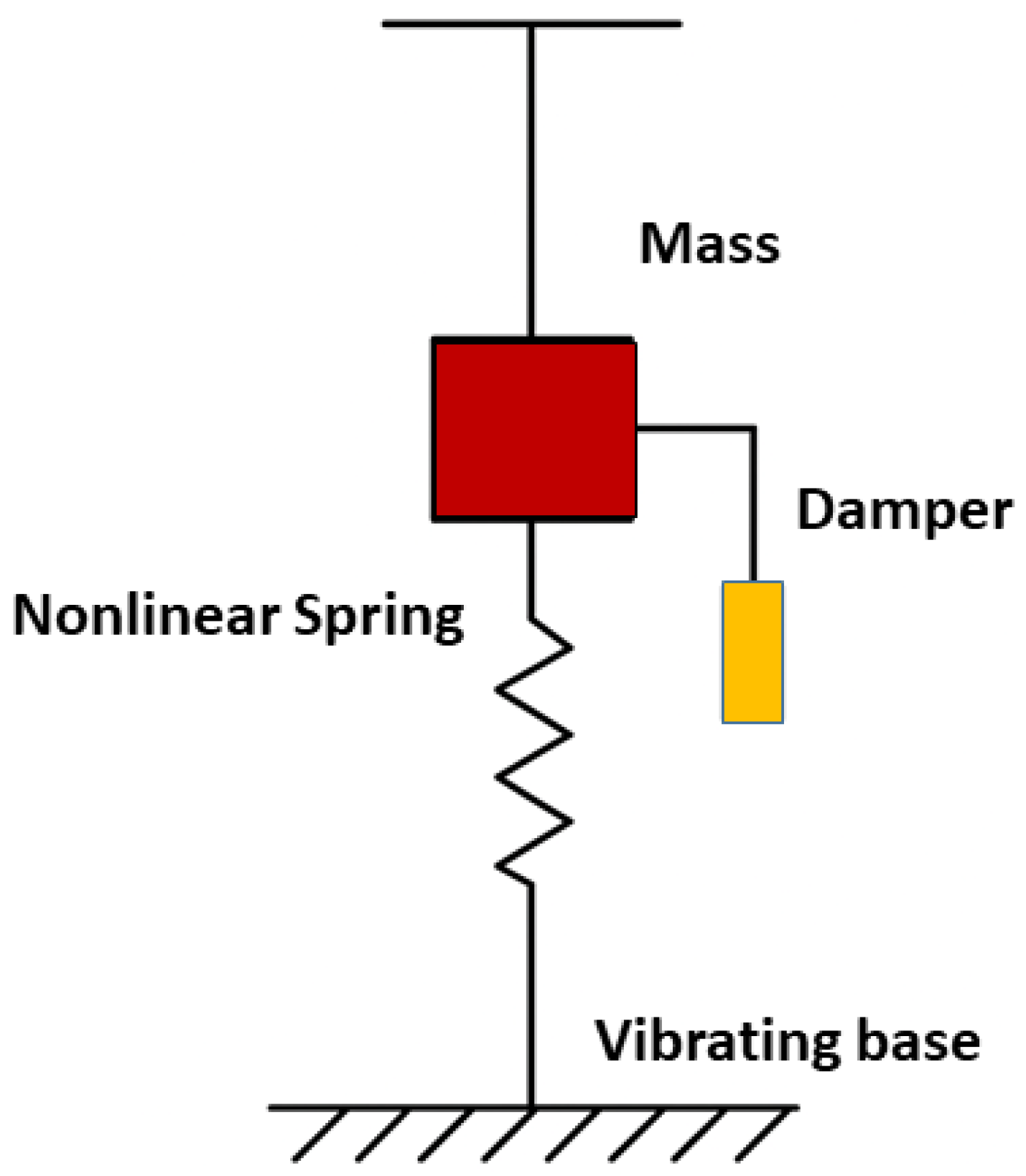
Figure 1. Schematic of the physical system modeled by the DM-CQDO equation. The damper provides linear damping ( Γ ), the nonlinear spring generates the linear, cubic, and quintic restoring forces ( η , Ξ , ϕ ), and the vibrating base introduces a parametric excitation by modulating the system’s stiffness at a frequency Ω .
Algorithms 18 00681 g001
Figure 2. Sparse identification. (a) Comparison of phase-space trajectories for the true system (blue, solid) and the SINDy identified model (red, dashed). (b) Time-series comparison for each state variable: y 1 ( t ) , y 2 ( t ) , and y 3 ( t ) . The near perfect overlap between the true (blue, solid) and identified (red, dashed) models confirms the predictive accuracy of the discovered equations.
Algorithms 18 00681 g002
Figure 3. Bifurcation diagrams for the DM-CQDO as a function of excitation frequency ( δ ) for six different damping coefficients ( γ ). Each panel depicts the local maxima of the displacement ( y 1 ) versus δ . The diagrams reveal a clear trend: increasing ( γ ) shifts the onset of chaos to higher frequencies and narrows the range of ( δ ) over which chaotic dynamics occur. At intermediate damping values ( γ = 0.25 ), a pronounced period-doubling cascade is evident, representing the primary route to chaos.
Algorithms 18 00681 g003
Figure 4. Stability diagrams for the DM-CQDO in the excitation frequency ( δ ) and amplitude (q) parameter space for three different damping coefficients: (a) low damping ( γ = 0.1 ), (b) intermediate damping ( γ = 0.25 ), and (c) high damping ( γ = 0.35 ). The color indicates the value of the LLE, with warmer colors (red/yellow) signifying chaos and darker colors (blue) signifying periodic or stable motion. The annotations highlight key dynamical features, such as the chaotic sea, periodic tongues, and bifurcation boundaries.
Algorithms 18 00681 g004
Figure 5. Lyapunov spectra for three different initial conditions: (a) y 1 = 0.01 , y 2 = 0.01 , y 3 = 0.01 , (b) y 1 = 0.3 , y 2 = 0.3 , y 3 = 0.3 , (c) y 1 = 0.5 , y 2 = 0.5 , y 3 = 0.5 . The plots illustrate variations in the largest Lyapunov exponent ( λ 1 ) across time, highlighting the system’s sensitivity to initial states. (a,b) show positive λ 1 , indicating chaotic behavior, while (c) shows a negative λ 1 , indicating stable, non-chaotic dynamics. This figure emphasizes the coexistence of multiple attractors and the influence of initial conditions on system stability.
Algorithms 18 00681 g005
Figure 8. Riddled basins of attraction with fractal boundaries. Each point on the grid represents an initial condition was iterated for 500 periods, colored according to the final attractor it converges to. The fine, interwoven structure of the basin boundaries is a hallmark of chaotic systems, visually confirming the system’s extreme sensitivity to initial conditions. Note how small changes in parameters across panels (af) significantly alter the basin geometry.
Algorithms 18 00681 g008
Figure 9. Phase-space trajectories of DM-CQDO under varying system parameters. (ac) Evolution of attractors with increasing damping coefficients γ = 0.003 , 0.03 , and 0.3 , respectively, illustrating the suppression of oscillatory behavior. (df) Influence of the parametric excitation frequency δ = 1.0 , 1.2 , and 1.5 , highlighting its role in destabilizing or sustaining periodic orbits. (gi) Effect of increasing nonlinear stiffness parameters ( L , M ) = ( 0.01 , 0.01 ) , ( 0.4 , 0.4 ) , and ( 1.5 , 1.5 ) , showing transitions from near linear to strongly nonlinear regimes. The trajectories are plotted in the phase plane ( y , y ) for fixed initial conditions, emphasizing the emergence of multi-stable behavior.
Algorithms 18 00681 g009
Figure 10. Chaotic attractors generated by varying parameters and initial conditions. (a) Chaotic attractor for parameters γ = 0.038 , n 1 = 2.05 , q = 4.01 , L = 0.08 , M = 0.65 , and δ = 0.2 with initial conditions [ 0.2 , 0.03 , 0.25 ] . (b) Chaotic attractor with the same initial conditions but modified parameters: γ = 0.048 , n 1 = 2.75 , q = 4.1 , L = 0.28 , M = 0.065 , and δ = 0.22 . The attractor expands significantly due to increased cubic nonlinearity. (c) Chaotic attractor with the same parameters but different initial conditions: [ 0.02 , 0.06 , 0.05 ] .
Algorithms 18 00681 g010
Figure 11. Return maps of the dynamical system are presented for fixed parameters L = 12.0 , M = 70.0 , and γ = 0.03 , while varying the frequency parameter δ across values δ = 2.7 , δ = 9 , δ = 15 , and δ = 30 .
Algorithms 18 00681 g011
Figure 12. Power spectra for three different initial conditions: (a) y 1 = 1.0 , y 2 = 0.0 , y 3 = 0.01 / 0.1 / 1.1 , (b) y 1 = 0.7 , y 2 = 1.0 , y 3 = 0.01 / 0.1 / 1.1 , and (c) y 1 = 0.2 / 0.4 / 0.6 , y 2 = 0.0 / 0.5 / 1.0 , y 3 = 0.05 / 0.15 / 0.5 , illustrating variations in power distribution across frequencies and highlighting the influence of initial states on spectral characteristics.
Algorithms 18 00681 g012
Figure 13. Recurrence plots reveal the system’s intricate dynamics, showcasing transitions between periodic and chaotic behavior. The diagonal lines and scattered points highlight sensitivity to initial conditions and the complexity of the attractors.
Algorithms 18 00681 g013
Table 1. System parameters, associated dynamics, and physical interpretations in a nonlinear parametrically excited system.
Parameter (Symbol)Observed DynamicsInterpretation
Displacement (Z)Varies with system responseSystem state variable representing position
Damping ( Γ )Limits oscillation amplitude, affects stabilityEnergy dissipation; influences limit cycles and routes to chaos
Linear stiffness ( η )Defines natural frequencyBase linear restoring force
Excitation amplitude ( ζ )Can induce parametric resonanceStrength of time-periodic stiffness modulation
Excitation frequency ( Ω )Controls timing of parametric excitationRate of stiffness modulation
Cubic nonlinearity ( Ξ )Causes hardening/softening, jump phenomenaDuffing-type effect: frequency hysteresis, multi-stability
Quintic nonlinearity ( ϕ )Adds further complexity, more equilibrium pointsHigher-order restoring force, enhanced multi-stability
Table 2. Comparison of true vs. identified coefficients for the y ˙ 2 dynamic.
TermTrue CoefficientIdentified CoefficientPercent Error
y 1 −1.0−0.98011.99%
y 2 −0.2−0.169615.2%
y 1 3 −0.1−0.10929.2%
y 1 5 −0.01−0.001288.0%
y 1 cos ( y 3 ) 1.00.94805.2%
cos ( y 3 ) 0.0−0.0142
Note: The higher percentage errors in the smaller coefficients (like for y 1 5 ) are common and often have a negligible impact on the overall system dynamics, as demonstrated in the plots.
Table 3. Approximate critical values of the excitation frequency ( δ c ) at which chaotic behavior begins, for different damping coefficients ( γ ). Values are estimated from visual inspection of Figure 3.
Damping Coefficient ( γ )Approximate Onset of Chaos ( δ c )
0.10≈1.8
0.15≈1.8
0.20≈3.0
0.25≈3.2
0.30≈3.4
0.35≈3.6
Table 4. Parameters and initial conditions used in Figure 8.
FigureParametersFixed Initial ConditionInitial Grid Range
(a) γ = 0.0003, n 1 = 4.0, q = 8.0, L = 5.5, M = 4.5, δ = 0.07 y 2 ( 0 ) = 0 y 1 ( 0 ) [ 2 , 2 ] y 3 ( 0 ) [ π , π ]
(b) γ = 0.00025, n 1 = 4.2, q = 9.0, L = 5.8, M = 5.0, δ = 0.06 y 2 ( 0 ) = 0 y 1 ( 0 ) [ 2 , 2 ] y 3 ( 0 ) [ π , π ]
(c) γ = 0.00035, n 1 = 3.8, q = 10.0, L = 6.0, M = 4.0, δ = 0.08 y 2 ( 0 ) = 0 y 1 ( 0 ) [ 2 , 2 ] y 3 ( 0 ) [ π , π ]
(d) γ = 0.0004, n 1 = 4.1, q = 9.5, L = 6.2, R = 4.8, δ = 0.09 y 2 ( 0 ) = 0 y 1 ( 0 ) [ 2 , 2 ] y 3 ( 0 ) [ π , π ]
(e) γ = 0.0002, n 1 = 4.3, q = 11.0, L = 6.5, M = 5.2, δ = 0.05 y 2 ( 0 ) = 0 y 1 ( 0 ) [ 2 , 2 ] y 3 ( 0 ) [ π , π ]
(f) γ = 0.0003, n 1 = 4.4, q = 10.5, L = 6.8, M = 5.5, δ = 0.04 y 2 ( 0 ) = 0 y 1 ( 0 ) [ 2 , 2 ] y 3 ( 0 ) [ π , π ]
Disclaimer/Publisher’s Note: The statements, opinions and data contained in all publications are solely those of the individual author(s) and contributor(s) and not of MDPI and/or the editor(s). MDPI and/or the editor(s) disclaim responsibility for any injury to people or property resulting from any ideas, methods, instructions or products referred to in the content.