Article

Integrating Structured Time-Series Modeling and Ensemble Learning for Strategic Performance Forecasting

1
Department of Public Health, Wannan Medical College, Wuhu 241000, China
2
Department of Medical Information, Wannan Medical College, Wuhu 241000, China
3
MRC Biostatistics Unit, University of Cambridge, Cambridge CB2 1TN, UK
4
Department of Public Foundation, Wannan Medical College, Wuhu 241000, China
*
Authors to whom correspondence should be addressed.
These authors contributed equally to this work.
Algorithms 2025, 18(10), 611; https://doi.org/10.3390/a18100611
Submission received: 19 August 2025 / Revised: 25 September 2025 / Accepted: 26 September 2025 / Published: 29 September 2025
(This article belongs to the Topic Applications of NLP, AI, and ML in Software Engineering)

Abstract

Forecasting outcomes in high-stakes competitive spectacles like the Olympic Games, World Cups, and professional league championships has grown increasingly vital, directly impacting strategic planning, resource allocation, and performance optimization across a multitude of fields. However, accurate forecasting remains challenging due to complex, nonlinear interactions inherent in high-dimensional time-series data, further complicated by socioeconomic indicators, historical influences, and host-country advantages. In this study, we propose a comprehensive forecasting framework integrating structured time-series modeling with ensemble learning. We extract key structural features via two novel indices: the Advantage Index (measuring a competitor’s dominance in specific areas) and the Herfindahl Index (quantifying performance outcome concentration). We also evaluate host-country advantage using a Difference-in-Differences (DiD) approach. Leveraging these insights, we develop a dual-branch predictive model combining an Attention-augmented Long Short-Term Memory (Attention-LSTM) network and a Random Forest classifier. Attention-LSTM captures long-term dependencies and dynamic patterns in structured temporal data, while Random Forest handles predictions for unrecognized contenders, addressing zero-inflation issues. Extensive stability and comparative analyses demonstrate that our model outperforms traditional and state-of-the-art methods, exhibiting strong resilience to input perturbations, consistent performance across multiple runs, and appropriate sensitivity to key features. Our key contributions include the development of a novel integrated forecasting framework, the introduction of two innovative structural indices for competitive dynamics analysis, and the demonstration of robust predictive performance that bridges technical innovation with practical strategic application. Finally, we transform our modeling insights into actionable strategic insights. This translation is powered by interpretable feature importance rankings and stability analysis that rigorously validate the robustness of key predictors. These insights apply across multiple dimensions—encompassing advantage assessment, resource distribution, strategic simulation, and breakthrough potential identification—providing comprehensive decision support for strategic planners and policymakers navigating competitive environments.

1. Introduction

In recent years, forecasting outcomes in high-stakes competitions has drawn global attention, owing to its critical implications for resource allocation, strategic planning, and performance enhancement. Such forecasting tasks are inherently challenging due to the complex interactions among economic factors, historical legacies, and event-specific dynamics [1,2,3,4,5,6,7,8]. These problems limit the effectiveness of existing methods. Traditional statistical methods, such as Auto-regressive Integrated Moving Average Model (ARIMA), have difficulty in dealing with the nonlinear relationships of high-dimensional data, and decomposition methods such as Holt-Winters experience a sharp rise in computational complexity as dimensionality increases. Although Ordinary Least Squares (OLS) regression [2,6,9] is easy to implement and interpret, it often relies on exponential functions that disproportionately penalize low medal counts and fail to account for the large number of countries that have yet to win any medals, resulting in poor handling of zero-inflated data. With the rise in machine learning models, linear regression, support vector machines (SVMs) [9], and random forests (RFs) [10,11] have been applied to medal distribution prediction, but RFs do not adequately capture long-term temporal dependency patterns, and XGBoost and others are difficult to handle discrete events and zero-inflation data [12]. Long Short-Term Memory (LSTM) can solve the problem of vanishing or exploding gradients in traditional RNNs and has potential in the field of sports competition prediction, but the standard LSTM architecture performs poorly in handling the global Olympic dataset [13].
Compared to recent studies employing deep learning for prediction, the innovative framework proposed in this research demonstrates significant enhancements across multiple dimensions. Current research predominantly focuses on single models or static feature analysis—such as using only recurrent neural networks for time series or tree models for structured data [14]. However, these approaches often overlook the inherent phased and heterogeneous nature of competition prediction—namely, the fundamental differences in predictive logic and key influencing factors between past medalists and potential newcomers [15,16]. Furthermore, while previous work acknowledges the importance of feature engineering [17,18], studies rigorously estimating the host effect using a DiD approach while introducing novel metrics—such as the Advantage Index (quantifying a nation’s competitive edge in specific events) and the Herfindahl Index (measuring the concentration of medal sources)—remain scarce. Regarding model architecture, relying solely on LSTMs may fail to adequately capture the disruption caused by sudden events or critical junctures to long-term trends. The attention mechanism introduced in this study specifically enhances the model’s ability to focus on critical time points and events, aligning with the transparency principles of explainable AI [19]. Furthermore, addressing the challenge of zero-inflated data—where regression models often perform poorly [20,21]—this research adopts a classification approach to identify potential first-medalists, effectively complementing existing prediction paradigms.
In summary, our contributions are threefold:
We propose a hybrid Attention-LSTM and Random Forest model that achieves excellent performance in predicting Olympic medal counts. Through comprehensive stability analysis, the model demonstrates strong robustness to input perturbations, consistent outputs across multiple training sessions, and appropriate sensitivity to key features. By effectively capturing both long-term trends and short-term patterns in high-dimensional time-series data, the model significantly improves the handling of zero-inflation issues.
We introduce two novel indices—the Advantage Index and the Herfindahl Index—to characterize the structural features of national medal performance. Additionally, we apply a rigorous DiD analysis to quantitatively confirm the significant impact of the host-nation effect.
To support National Olympic Committees (NOCs) in strategic planning and resource allocation, we extract actionable insights across four dimensions: advantage assessment, resource distribution, strategy simulation, and breakthrough potential detection.

2. Related Works

High-dimensional time-series forecasting refers to the prediction of future values or states for time-series data containing multiple variables [22]. This type of data usually records information about multiple interrelated variables in the system over time, such as temperature, humidity, and wind speed in meteorological data, multiple stock prices in financial data, and gene expression in biological data [23]. In the prediction process, the dependencies between variables and the trend characteristics in the time dimension need to be captured through modeling, and commonly used methods include dimensionality reduction techniques [24], machine learning models [25], and deep learning methods [26]. The core challenge is to deal with the complex correlation between variables, the high dimensionality of data, and the dynamic evolution law [22,26].
Empirical studies analyzing the performance of various parties in high-risk competitive events can be broadly divided into five categories, using large-scale sporting events such as the Olympics as examples. The first category involves the analysis of macroeconomic and social variables. Most of the studies emphasize that macroeconomic and social variables such as national GDP and population size constitute the core drivers of the number of medals [1,2,3,4,5,6,7,8], and their theoretical basis lies in the positive correlation between the country’s resource endowment and sports achievements [27]. However, there are obvious limitations in the ability of this type of view to explain short-term economic fluctuations, specific historical events such as sudden political changes or impacts brought about by the host country, as well as dynamic changes at the level of specific sports. The second category consists of traditional time series models. Traditional time-series models such as the autoregressive integrated moving average model (ARIMA) have been applied to the time-series prediction of single-country medal counts [28], but their linear assumptions are difficult to effectively deal with the complex interactions and nonlinear correlation mechanisms among variables under the multinational competition system. The third category is classical regression methods. Many researchers have adopted ordinary least squares (OLS) regression due to its ease of interpretation [2,6,9]. However, predicting the number of Olympic medals faces various discrete events and zero-inflation problems: the method does not accurately reflect the future performance of countries that have not yet won any medals, and the number of these countries is very large.
The fourth category comprises machine learning approaches that treat each Olympic Games as an independent data point, incorporating temporal information through feature engineering. Their core strengths lie in capturing nonlinear interactions between features and providing interpretability. Their weakness is their inability to automatically model long-term temporal dependencies. With the rise in machine learning models, linear regression and SVMs have been applied to the practice of predicting medal distributions by constructing feature hyperplanes [9]. RF has gained empirical applications in dealing with multidimensional feature interactions and nonlinear relationship modeling by its integrative learning properties and ability to quantify feature significance for tasks such as predicting the outcome of soccer matches [4] or horse racing results [10,11], but the model is still insufficient in capturing the long-term temporal dependency patterns spanning across multiple Olympic cycles. As integrated learning methods based on decision trees, both XGBoost and Random Forest excel at handling nonlinear relationships and feature interactions, yet struggle to effectively model discrete and zero-inflation data. This means that these algorithms may not be able to accurately capture truncation points or zero-value generating mechanisms in the data, leading to prediction bias [12].
The fifth category comprises deep learning methods that treat data as continuous time series, with their core advantage being the automatic capture of temporal dependencies. Their evolved model, Attention-LSTM, further enhances the ability to focus on critical time points, thereby better handling discrete events and local mutations. LSTM effectively solves the common problem of gradient vanishing or explosion in traditional RNNs when dealing with long sequential data, based on the advantages of their gating mechanisms for modeling long-time dependencies. These gating mechanisms enable LSTM to dynamically control the information flow and selectively memorize or forget relevant information. It has shown significant potential in the field of sports competition prediction, including event result extrapolation and athlete performance evaluation [13]; however, the standard LSTM architecture may have difficulty in dynamically focusing on the information mutations at key time nodes when dealing with global Olympic datasets with significant local temporal aggregation features by its fixed time window mechanism, which results in poor performance in some cases and prevents the accurate assessment of the impact of discrete events.
With the popularity of the Transformer architecture, the attention mechanism was introduced into LSTM in order to solve this problem, so that the model can focus more on the important parts. By integrating the strengths of both the fourth category and the fifth category models, we employ a Random Forest classifier to leverage its ability to handle zero-inflation issues, addressing the classification task of “whether an award is received for the first time.” We combine this with Attention-LSTM to harness its capacity for capturing long-term temporal dependencies and focusing on key events, thereby tackling the regression task of “how many awards are received.” The model incorporates time series trend analysis and machine learning features. It excels in solving the long-term dependency problem in time series data and can effectively focus on the impact of short-term discrete event features.

3. Materials and Analysis

3.1. Assumptions and Notations

3.1.1. Assumptions and Justifications

Final medal totals are usually not based on historical medal totals but rather relate to current athletes who will be competing at the Olympic Games. While historical data can provide some references, factors such as an athlete’s strength, condition, and preparation can directly affect the final medal count. Thus, even if a country has performed well in the past, it may not achieve the same number of medals if the current lineup of athletes is not strong enough.
Olympic data from the Soviet Union and Russia can be interconnected, as can Olympic data from East Germany, West Germany, and Germany. After the collapse of the Soviet Union, Russia inherited most of the Soviet Union’s sports resources and athlete base, so there is some continuity in its Olympic data. Similarly, East and West Germany formed modern Germany after reunification, and their sports data can be merged.
Countries’ participation experience can be accumulated in dominant sports. Before winning their first medal, athletes and coaching teams accumulate experience in technical enhancement, tactical scheduling, and adapting to competitive environments. When a country has been involved in a sport for a long time, this experience lays the groundwork for subsequent medal breakthroughs, even if they are not won initially. Dominant sports are often the focus of national sports systems.

3.1.2. Notations

The primary notations used in this paper are listed in Table 1.

3.2. Feature Extraction

3.2.1. Characterization 1: Advantage Sport Effect

First, to explore in depth the extent of a country’s advantage over other countries in a sport, we assume that the proportion of medals won by a country in a given sport to the total number of medals awarded in that sport constitutes the Advantage Index of that country in that sport. The higher the Advantage Index, the more significant the competitive advantage of that country in that sport. We introduce an indicator, the Advantage Index, whose formula is shown in Equation (1).
Let the country be i and the sport be j . Then, the Advantage Index A i j is defined as:
A i j = M i j k M k j ,
where M i j is the total number of medals won by the country in the project. M k j is the number of medals won by country k in event j . k M k j is the total number of medals won globally in event j . A i j quantifies the relative dominance of country i in project j , with a value range of [0, 1], enabling us to more comprehensively evaluate the performance of other countries in various sports projects and thereby reveal their respective areas of strength.
Second, to illustrate which sport has a more critical impact on a country than others. As shown in Equation (2), we use the Herfindahl Index to measure concentration [29].
H i = j M i j T i 2 ,
where T i is the total number of medals won by the country i .
The larger the Herfindahl Index is for a country, the greater the concentration of medals it has won in each event. If a country’s medals are concentrated in a few events, then its H i will be greater than 0.5, which is a high Herfindahl Index; if a country’s medals are more evenly distributed, then its H i will be less than 0.3, which is a low Herfindahl Index.
Third, as shown in Figure 1, combining the two indicators makes it possible to determine which sport is more important for different countries and how the advantageous sport affects the number of medals won by a country.
China shows great advantages in Swimming, Athletics and Badminton, with a very high dominance in Badminton (54.35%). The Herfindahl Index of 0.83 indicates that China’s medal distribution is highly concentrated in a few advantageous sports, which reflects China’s strong competitiveness in these sports.
The United States has an absolute advantage in swimming and track and field, which accounts for almost 80% of its total medals. Basketball is also its traditional strength. Herfindahl Index of 0.36 shows that the U.S. medal distribution is relatively concentrated in a few sports.
Great Britain is strong in cycling and rowing, but its advantage is less pronounced than that of the United States and China. Although not accounting for a high proportion of the total, the equestrian events are also one of its traditional strengths. Herfindahl Index of 0.12 indicates Britain’s medal distribution is relatively decentralized, with no prominent advantage in sports.
Japan has a significant advantage in Judo and Gymnastics, especially in Judo, which accounts for 34.38% of the global medals in this category. A Herfindahl Index of 0.19 indicates Japan’s medal distribution is relatively spread out, but Judo and Gymnastics are still its core strengths.
France is a strong performer in fencing, cycling and equestrian, especially in fencing, which has 32.56% of the world’s medals, with a Herfindahl Index of 0.17, suggesting that France’s medal distribution is more spread out, but fencing is still its most significant strength.
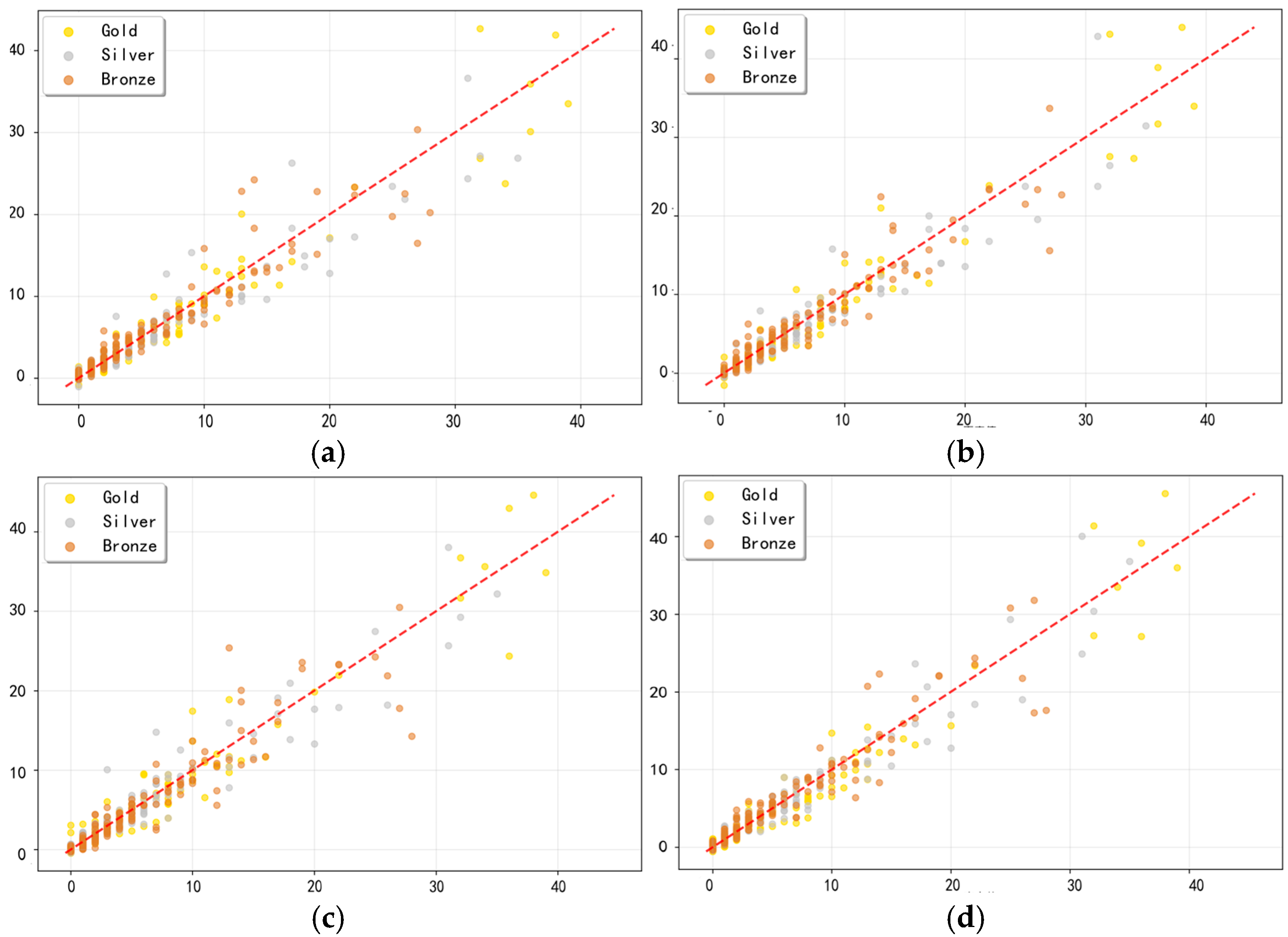
Additionally, we conducted ablation experiments for these two metrics, as shown in Figure 2. We removed each metric separately to observe their impact on prediction results. The results revealed that removing A i j reduced RMSE by 1.37%; removing H i increased RMSE by 3.25%; and removing both features simultaneously reduced RMSE by 4.77%. Detailed data are presented in Table 2. In summary, although their impact is relatively limited, both features make positive contributions to the model and are worth retaining. We will further analyze all metrics in the Methods section.

3.2.2. Characterization 2: Host Country Effect

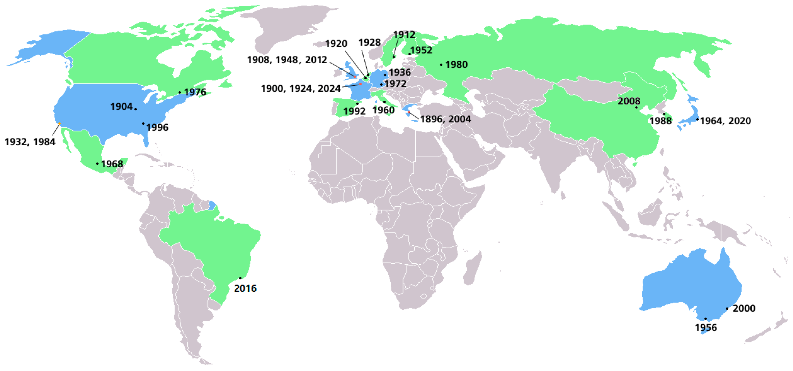
First, when exploring the medal data distribution patterns of Figure 3, we note a striking phenomenon: It shows striking similarities to that in Figure 4.
In Figure 4, countries that have hosted one Summer Olympics are identified in green, while those that have hosted two or more are identified in blue. Based on this finding, we delve further into whether there is some potential correlation between being a host country and the number of medals won.
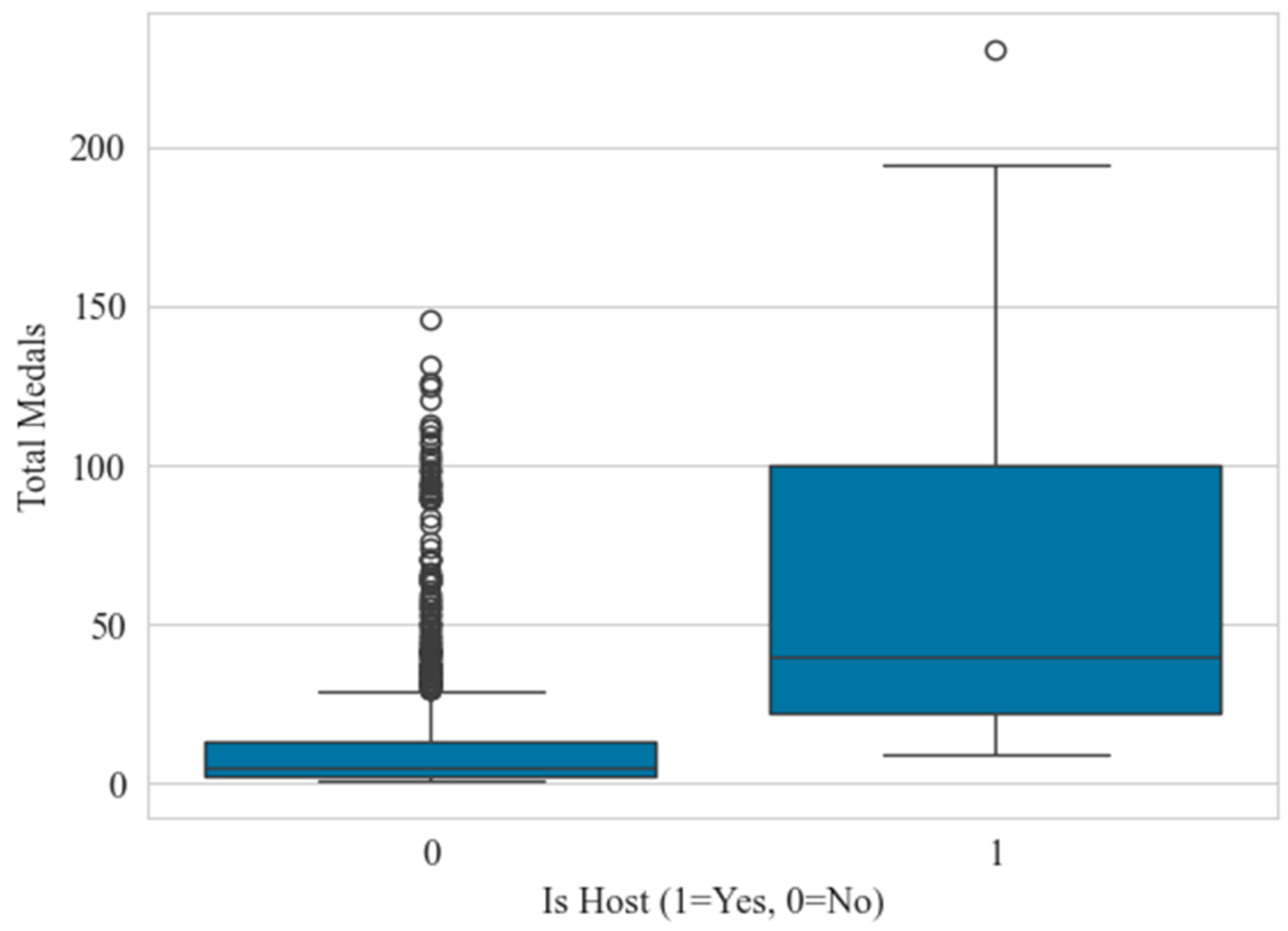
Second, as shown in Figure 5, we conduct an in-depth analysis using the DiD, constructing a dichotomous variable to identify the host country and its special status in the preceding and following periods. The results of the study clearly show that when the same country is the host country, it wins significantly more awards than in the non-host country period. This finding reveals the positive effect that host country status may have on the number of awards received. We formally implement the DiD methodology through the following econometric specification:
Y i t = β 0 + β 1 · H o s t i t + β 2 · P o s t i t + β 3 · ( H o s t i t × P o s t i t ) + γ X i t
where Y i t denotes the medal count for country i   in year t , H o s t i t   is a binary indicator for host country status, P o s t i t   marks the post-hosting period, and X i t   represents control variables, including GDP and population. The coefficient β 3 captures the causal effect of hosting, identified under the parallel trends assumption verified through pre-event data diagnostics shown in Figure 5.
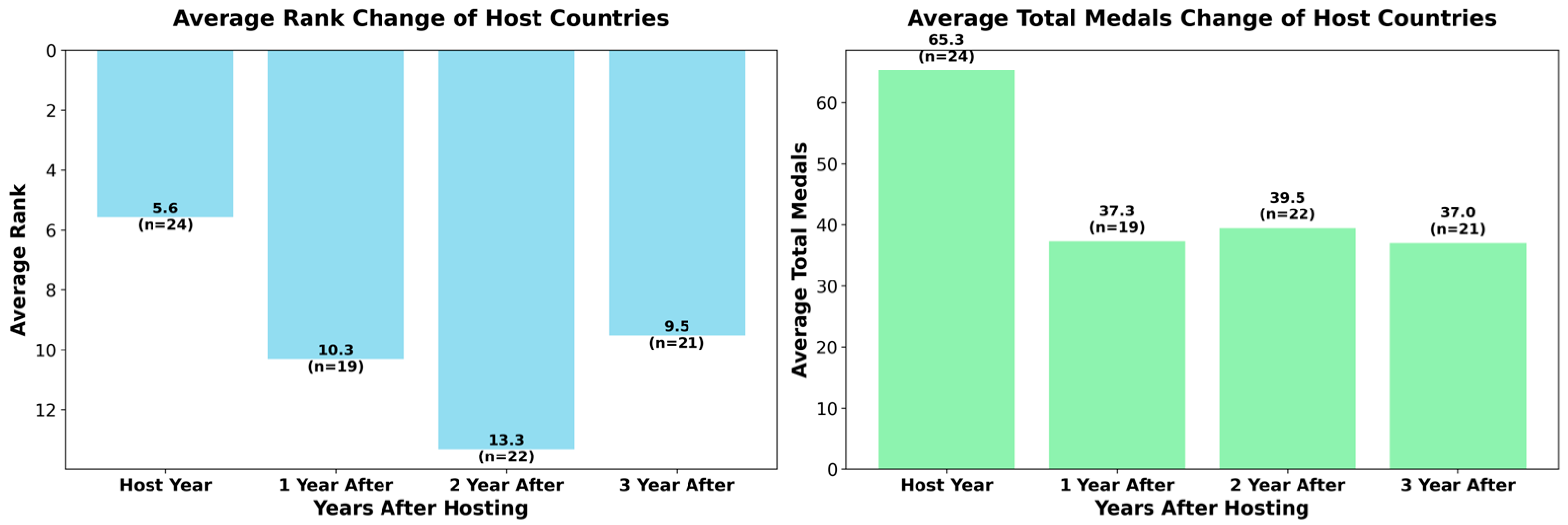
Third, we examine the short-term and long-term impacts of the host nation effect. Host nations typically enjoy significant advantages, which may be leveraged through proposals to add new sports or events. But is this advantage sustainable? As shown in Figure 6, this study compares the host nation’s performance during the current Olympics with its results in the subsequent three editions. It is evident that the host nation’s performance significantly improves in the hosting year but rapidly declines thereafter. This striking finding prompts deeper reflection: although host nations often favor adding events that leverage their national strengths during selection, these advantages do not necessarily translate into significant impacts in subsequent Olympic Games.

3.2.3. Feature Engineering

Combining the data preprocessing and characterization above, we focus our feature engineering on the dominant SPORT and host country effects. Feature engineering is further enhanced by creating binary variables to identify whether a country is a current or future host country and using lagged variables to count the number of medals won by each country in dominant sports in the previous 1–3 Olympics. Next, we customize a PyTorch 1.12.0 dataset class to facilitate the encapsulation of the input time series data and target values into an iterable dataset object. Finally, the features are normalized to ensure that features with different value ranges do not adversely affect the model training, thus improving the stability and accuracy of the model.

4. Methods

4.1. Model Notations

The notations are listed in Table 3 to formalize the model structure and mathematical formulations throughout this section.

4.2. Model Structure

To address both repeat and first-time medalist forecasting, we build a dual-branch model combining an Attention-LSTM module and a Random Forest classifier. As shown in Figure 7, we divided the task of predicting the entire medal table into predictions for non-first-time medal-winning countries in the red section and predictions for first-time medal-winning countries in the yellow section, and integrated them to obtain a model for predicting the number of Olympic medals won by each country.
In the red area, we show the construction of the model for predicting countries that are not first-time medal winners. We analyze the importance of each country in each sport, which is quantified as the dominant sport; at the same time, we examine the impact of the sport chosen by the host country on the final outcome, which is quantified as the host country effect. In order to better capture the data trends, we introduced the attention mechanism and constructed an attention-LSTM model. Focusing on the main project effect and the host country effect, the feature engineering was trained and validated. After validating the model performance metrics and stability analysis, we ensure the reliability of the model.
In the yellow area, we show the process of constructing a predictive model for a country winning a medal for the first time. We considered the historical number of participants, the number of athletes, participation in dominant sports and other metrics, and used a random forest classifier to predict the likelihood of all non-winning countries winning a medal.

4.3. Prediction Model for Non-First-Time Medal-Winning Countries

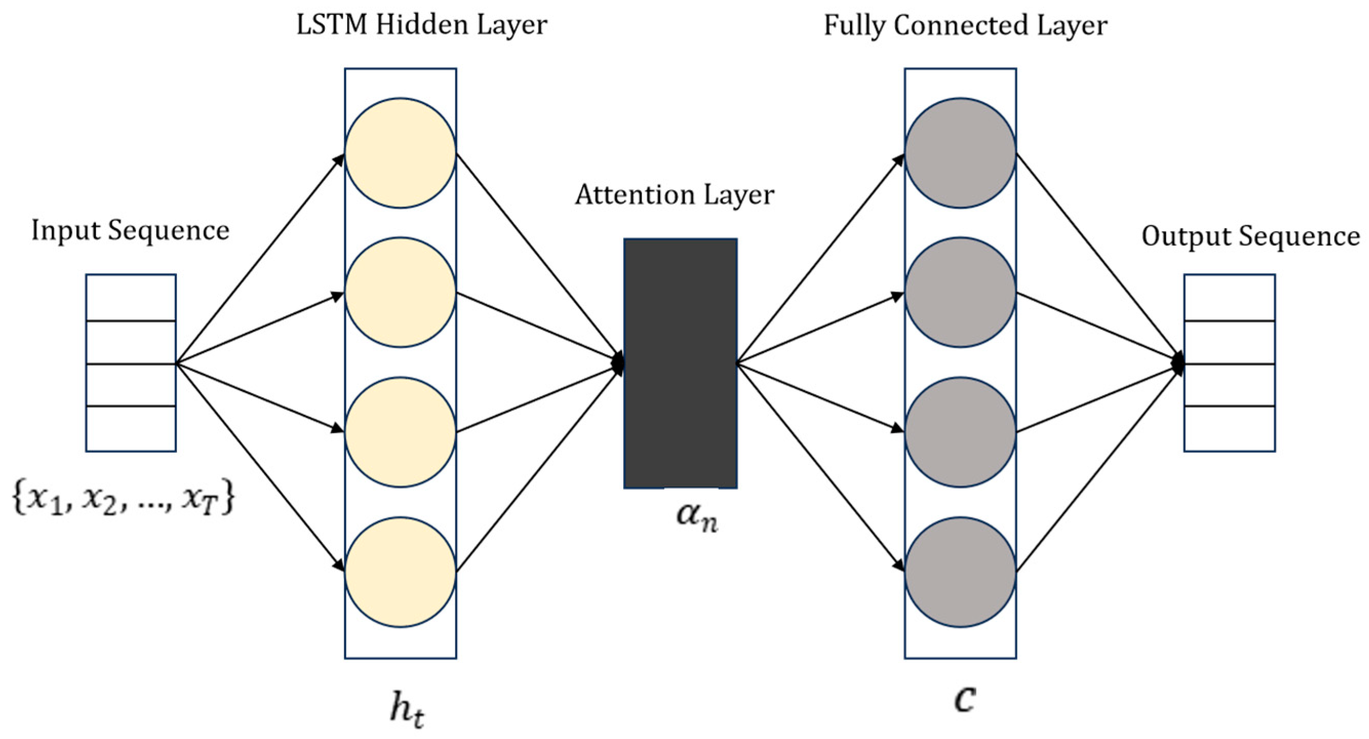
As shown in Figure 8, we use an attention-enhanced LSTM (Attention-LSTM) model, which consists of three core components. The LSTM layer captures long-term temporal dependencies through a gating mechanism. The attention layer dynamically weights the importance of historical moments. The fully connected layer maps to the final prediction result.
Let the input sequence be x 1 , x 2 , , x T . The calculation process at time step t is as follows:
1.
LSTM gating calculation
i t = σ W i i x t + b i i + W h i h t 1 + b h i
Equation (4) is the input gate i t , where i t compresses the input value to the [0, 1] interval through the Sigmoid function σ to achieve a gating effect. Among them, W i i x t processes the current input features, W h i h t 1 fuses historical hidden states, and the bias term b enhances the flexibility of the model. The closer the final output value is to 1, the more important the current information is, thereby controlling the proportion of new information flowing into the cell state c t .
f t = σ W i f x t + b i f + W h f h t 1 + b h f
Equation (5) is the forgetting gate f t , which determines the degree of retention of historical information. Its structure is symmetric to the input gate but complementary in function. W h f and b h f extract historical memory features, while W i f and b i f associate the current input. After Sigmoid activation, they generate the forgetting coefficient. When f t approaches 1, historical memory is fully retained; when f t approaches 0, historical information is cleared, effectively alleviating the vanishing gradient problem.
o t = σ W i o x t + b i o + W h o h t 1 + b h o
Equation (6) is the output gate o t , which controls the degree of information exposure of the hidden state h t . The dual linear transformations W i o , b i o , W h o , and b h o fuse spatio-temporal features and generate a gated vector through σ . This mechanism enables the model to dynamically select the memory content to be output, such as highlighting the impact of data from key years in medal predictions.
c t ~ = t a n h W i c x t + b i c + W h o h t 1 + b h c
c t = f t c t 1 + i t c t ~
Equations (7) and (8) illustrate the update mechanism of the memory cell c t . Candidate memories c t ~ are used to generate new memory proposals in the range [−1, 1] using the tanh activation function. Memory update employs gated weighted summation: f t c t 1 achieves selective forgetting of historical memories, while i t c t ~ achieves selective absorption of new information.
h t = o t t a n h c t
Subsequently, Equation (9) outputs the current hidden state. The output of the LSTM hidden layer is passed to the Attention layer.
2.
Attention mechanism
α n = exp s x n , q j exp s x j , q
Equation (10) implements the calculation of temporal attention weights. The scoring function s x n , q = v T tanh W h h t + W q q is used to measure the similarity between the input state x n and the query vector q . This context vector c is concatenated with the final LSTM output and passed through a fully connected layer to generate the final prediction of medal counts (gold, silver, bronze) in Equation (11).
c = n α n h n
This attention-enhanced LSTM architecture improves model interpretability and predictive accuracy, particularly when handling non-stationary data and temporal disturbances. Unlike traditional time series models such as ARIMA or even standard LSTMs, the attention mechanism explicitly quantifies the contribution of each historical time step. For instance, it assigns higher weights to Olympic cycles with similar host country backgrounds or sudden shifts in dominant events. This transparency not only builds trust in the predictions but also delivers actionable insights—such as identifying which historical events most significantly influence future medal outcomes.

4.4. Prediction Model for First-Time Medal-Winning Countries

For countries that have yet to win an Olympic medal, we addressed the severe category imbalance—where first-time medal-winning nations constitute a disproportionately small sample—through the following approaches: (1) Generating synthetic positive samples using SMOTE (Synthetic Minority Over-sampling Technique); (2) Adjusting class weights inversely proportional to sample frequency within the random forest classifier. This ensures the model avoids bias toward majority classes and enhances recall for potential first-time medalist candidates.
Next, we constructed a predictive model to identify which nations are most likely to win their first medal at the 2028 Los Angeles Olympics, providing confidence intervals for the predictions. Predicting whether a country will win its first medal at a specific Olympics is a binary classification problem. Therefore, the target variable is binary-coded: countries winning their first medal are coded as 1, and those not winning their first medal are coded as 0. To build an efficient and accurate predictive model for identifying potential first-time medal-winning nations, we selected the following key features and defined their symbolic representations:
  • Historical Number of Entries ( H i ): Defined as the number of times country i has competed in previous Olympic Games ( H i Z + ).
  • Number of Athletes ( A i c u r r ): Defined as the number of athletes sent by country i in the current Olympics ( A i c u r r Z + ).
  • Advantage Sport Participation ( P i a ): A binary indicator representing country i’s participation in sports identified as its advantage areas (e.g., track and field, swimming, etc.) in the current Olympics ( P i a { 0 , 1 } ).
  • Number of Medals Won by Neighboring Countries ( M i n e i g h ): Defined as the sum of medals won by countries geographically or economically clustered around country i in the current Olympics ( M i n e i g h Z + ), reflecting potential clustering effects.
These characteristics are instrumental in enabling the model to capture a country’s latent potential for securing its inaugural medal. For instance, countries with a higher historical participation count H i inherently possess greater developmental opportunities for future breakthroughs. Furthermore, active engagement in recognized advantage sports P i a and the competitive momentum reflected in neighboring nations’ medal tallies M i n e i g h provide valuable signals of the country’s current competitive standing and external influences.
Third, the Random Forest Classifier is selected as the prediction model due to its exceptional capabilities as an integrated learning method. This approach demonstrates strong robustness when handling outliers and noisy data, while simultaneously enabling effective evaluation of feature importance through built-in significance assessment mechanisms. Furthermore, the model exhibits superior capacity in capturing complex nonlinear feature interactions [31]. Collectively, these characteristics enhance the stability and efficiency of our prediction framework when processing diverse and complex datasets.
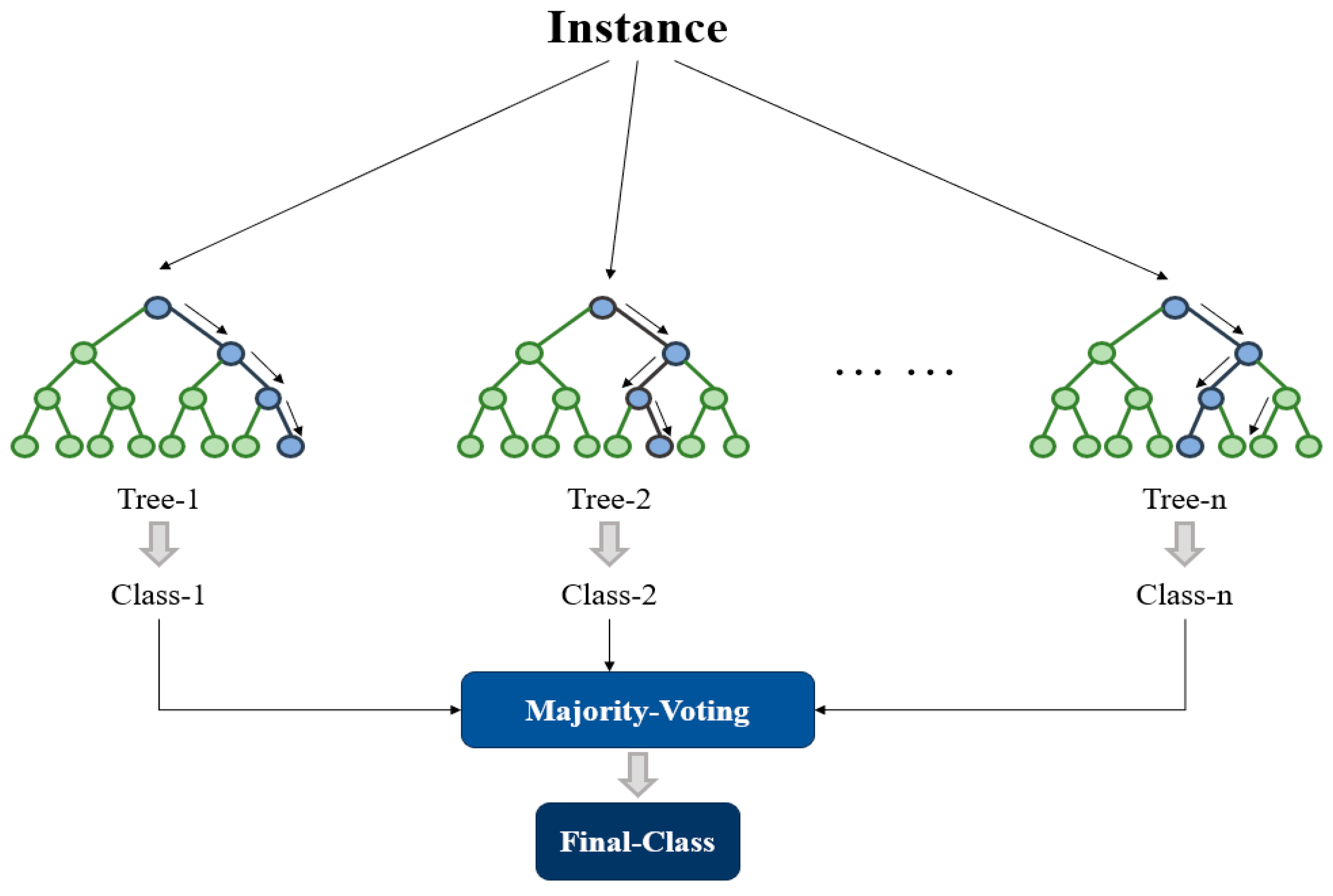
As shown in Figure 9, We randomly select some samples from the dataset as the training set for each decision tree. At each split node, the square root d features are randomly chosen from all features   d . After constructing each decision tree based on the sampled data and candidate features and deciding to grow the tree to the maximum depth, the final prediction result is derived by Majority Voting, i.e., the category with the highest number of occurrences among all the decision tree predictions is selected as the final prediction category.

4.5. Explainability Analysis

Although deep learning models demonstrate outstanding predictive performance, their “black box” nature limits their application in critical decision-making scenarios. To enhance model credibility and practicality, this study employs the SHAP (SHapley Additive exPlanations) method to conduct interpretability analysis on the Attention-LSTM Olympic medal prediction model. Based on the Shapley value from game theory, SHAP assigns fair contribution values to each feature, providing transparent explanations for model decisions [32].

4.5.1. Theoretical Foundations of SHAP

The SHAP method is based on the following core principles: Additivity, where the sum of SHAP values for all features equals the difference between the model prediction and the baseline value; Symmetry, where features contributing equally to the prediction result have identical SHAP values; Virtuality, where features contributing nothing to the prediction result have SHAP values of zero; Monotonicity, where the direction of change in SHAP values aligns with the direction of change in model output as feature values increase.
For the Attention-LSTM model in this study, SHAP values are calculated as follows:
ϕ i = S F i | S | ! ( | F | | S | 1 ) ! | F | ! [ f ( S { i } ) f ( S ) ] ,
where ϕ i represents the SHAP value for the feature i , F denotes the set of all features, S indicates the feature subset excluding the feature i , and f ( S ) signifies the model prediction value using the feature subset.

4.5.2. Analysis of the Model Decision-Making Process

To gain a deeper understanding of the model’s decision-making process, this study employs SHAP waterfall plots to provide detailed explanations for individual predictions. These plots clearly illustrate the contribution path of each feature to the final prediction outcome, starting from the baseline value and progressively accumulating the SHAP values of each feature until the final prediction result is reached.
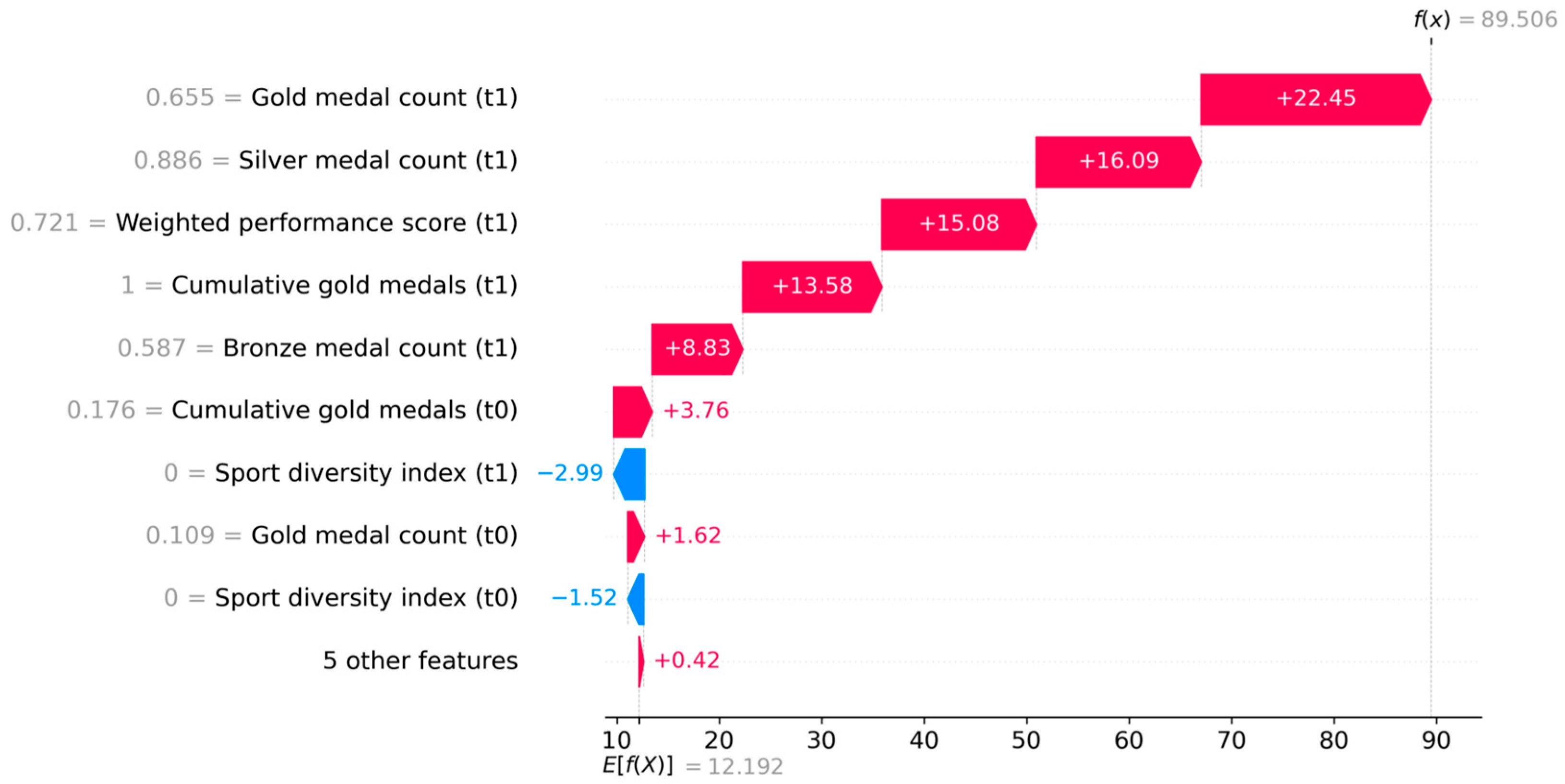
Through SHAP waterfall chart analysis, we conducted an in-depth exploration of the model’s decision-making mechanisms across different prediction scenarios. Figure 10 illustrates the feature contribution patterns for the high medal prediction sample, where the Gold medal count (t1) demonstrated the strongest positive impact (23.438), aligning with the expectation that gold medal count serves as the most direct indicator for predicting future performance. Subsequently, the Silver medal count (t1) (15.346) and Weighted performance score (t1) (15.000) contributed significantly, collectively forming a robust positive contribution portfolio. Notably, all major features showed positive contributions, elevating the prediction value from the baseline of 12.192 to the final predicted value of 89.506, indicating that the model identified consistent high-performance indicator patterns in high medal predictions.
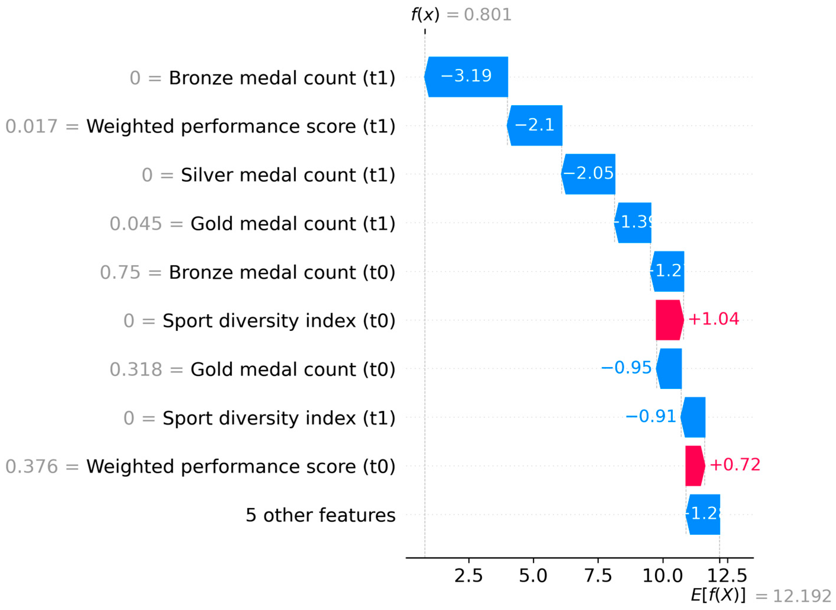
In contrast, the low medal prediction sample in Figure 11 exhibited significant negative contribution patterns. The bronze medal count (t1) showed the largest negative contribution (−3.190), forming a stark contrast with the high medal sample and reflecting a severe shortage of historical bronze medal counts. Subsequently, the weighted performance score (t1) (−2.104) and silver medal count (t1) (−1.993) demonstrated significant negative contributions, reducing the predicted value from the baseline of 12.192 to the final prediction of 0.801. This pattern indicates that the model identified critical deficiencies in multiple key indicators during low medal predictions.
The comparative analysis reveals hierarchical decision-making characteristics: the model first establishes foundational predictions through core indicators like medal count, then performs fine-tuning using comprehensive metrics. In high-medal samples, coordinated effects from all indicators create cumulative positive impacts, elevating predictions to 7.3 times the baseline value, whereas in low-medal samples, negative indicators dominate, reducing predictions to 0.07 times the baseline. Additionally, the importance of t1 (current time step) features consistently outweighs t0 (previous time step) characteristics, validating the model’s capability to effectively capture temporal dynamic patterns in Olympic medal predictions.

4.5.3. Interpretation of Feature Importance

The feature importance analysis results based on SHAP values are shown in Table 4.
Overall, gold, silver, and bronze medals accounted for three of the top four positions, collectively representing 65.3% of the total. This underscores the importance of continuity and historical performance in competitive sports. This finding aligns closely with the reality of athletic competition, where past achievements often serve as the strongest predictor of future performance. The Advantage Index ranks third (importance score: 1.5006), reflecting the significant influence of a nation’s overall sports development level on medal predictions. This indicator encompasses not only competitive prowess but also multiple dimensions such as sports infrastructure and talent development systems. Is_Host scored only 0.1366, ranking last, indicating the host nation advantage plays a relatively limited role in long-term predictions. This may stem from the host advantage primarily manifesting during the current Olympic Games, exerting minimal influence on subsequent editions.

5. Experiments

5.1. Data Preparation and Preprocessing

This study utilizes publicly available Olympic datasets curated by COMAP, encompassing five core data categories essential for comprehensive analysis. The dataset includes historical records of all summer Olympic athletes detailing their sports disciplines, participation years, and competition outcomes. Complete national medal distribution tables span every summer Games from 1896 to 2024, while host nation documentation covers the period from 1896 to 2032. Additionally, event program statistics quantify discipline-specific and total event counts across all summer Olympiads, supplemented by descriptive metadata providing contextual explanations and usage examples.
To establish a robust foundation for analysis, we implement a comprehensive data preprocessing pipeline encompassing four critical stages. Initial integration combines medal distribution records, host nation designations, and event program statistics through temporal and national alignment, enabling comprehensive Olympic performance profiling while specifically extracting non-medal-winning country datasets. Subsequent cleaning addresses historical geopolitical complexities by standardizing national identifiers—such as consolidating Soviet Union records under Russia’s current designation and unifying East/West Germany entries—ensuring temporal coherence across the century-spanning dataset. Explicit host nation labeling is then applied to each Olympiad using official records, creating essential variables for subsequent advantage quantification. Finally, autocorrelation diagnostics validate inherent temporal structures within the processed dataset, confirming non-random patterns before modeling.
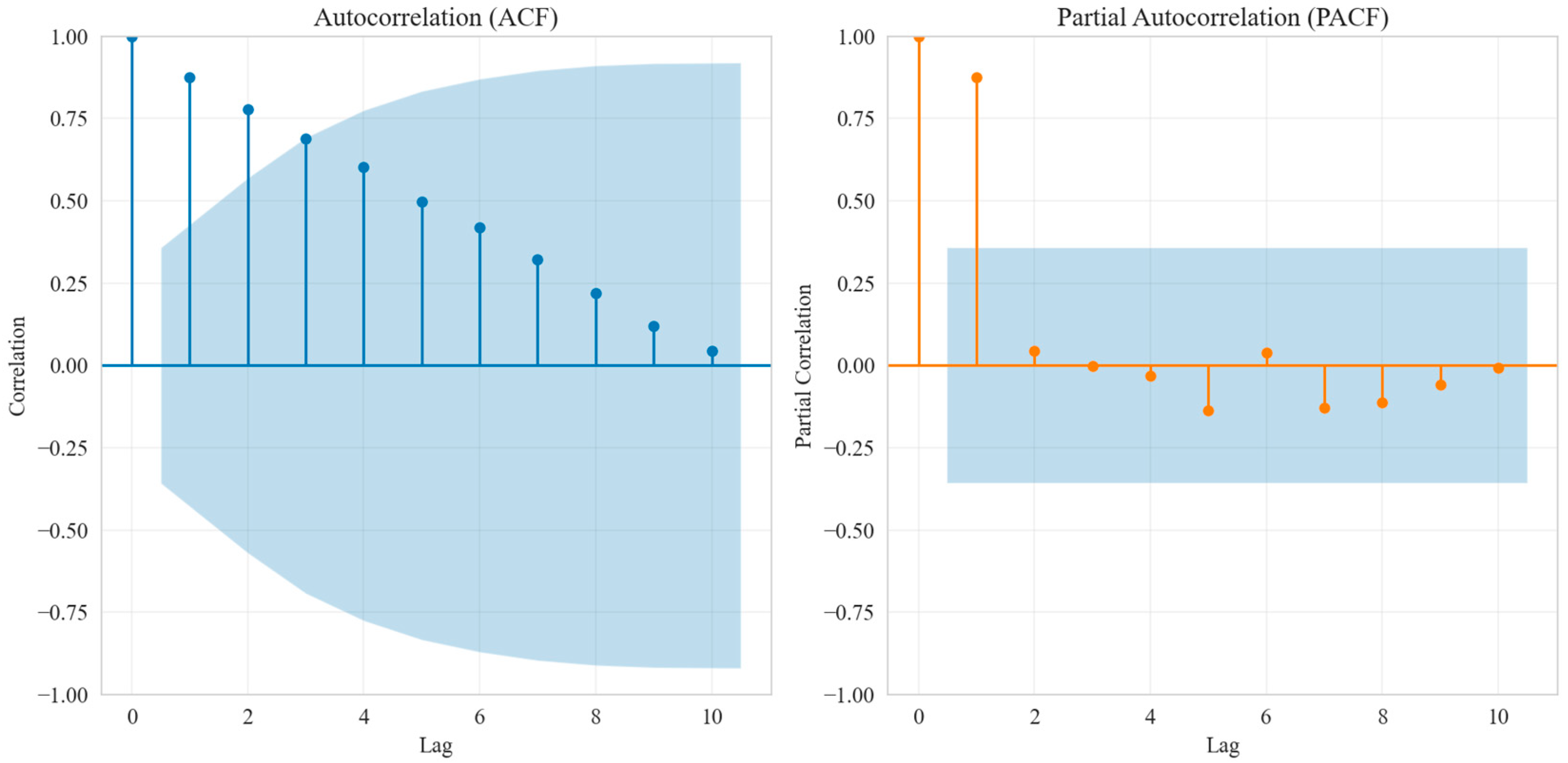
As shown in Figure 12, by plotting the AutoCorrelation Function (ACF) and Partial AutoCorrelation Function (PACF), we provide a detailed demonstration of the autocorrelation coefficients and partial autocorrelation coefficients at different lag orders. The results clearly show that the data exhibit significant partial autocorrelation, implying some underlying pattern or trend within the data rather than a completely random distribution. For further analysis and prediction, we divide the dataset into the training set and the test set according to a ratio of 8:2 to verify its validity and accuracy in the subsequent model training and testing process.
Although this study utilizes Olympic-related datasets for demonstration, our data preprocessing pipeline—including merging, cleaning, and normalization steps—is broadly applicable to any high-dimensional structured dataset.

5.2. The Model Training

To ensure the stability and convergence of model training, we performed MinMax normalization on all numerical features. This normalization method maps feature values to the [0, 1] interval, effectively eliminating differences in scale between different features and laying the data foundation for subsequent deep learning model training. Considering the quadrennial nature of the Olympic Games, we reconstruct the temporal sampling strategy to align with Olympic cycles. Specifically, historical data from the last three Olympic editions (spanning 12 years) is used as the input sequence to predict medal distributions for the upcoming Olympics. This ensures temporal coherence with the 4-year Olympic periodicity while maintaining sufficient historical context for pattern recognition.
The Attention-LSTM model designed in this study comprises three core components. The LSTM layer is responsible for capturing long-term dependencies in the time series, effectively addressing the vanishing gradient problem through gating mechanisms, and providing rich hidden state representations for subsequent attention calculations. The attention mechanism calculates the importance of weights for each time step, enabling the model to adaptively focus on the most relevant historical information for the prediction task. The specific implementation includes attention weight calculation, context vector generation, and a fully connected output layer. The fully connected output layer uses a two-layer fully connected network to map the output of the attention mechanism to the final medal prediction results, where the ReLU activation function introduces a nonlinear transformation to enhance the model’s expressive capability.
Our hyperparameter settings are shown in Table 5. It settings were determined through a two-stage optimization process: first, a grid search over candidate ranges (learning rate: 0.0001–0.01, hidden size: 32–256) using 5-fold cross-validation on the training set, followed by fine-tuning via Bayesian optimization to minimize validation loss. In the final validation phase, the model evaluates performance on the validation data, with early stopping triggered if loss does not improve for 20 consecutive epochs to prevent overfitting.
This study employs the mean square error (MSE) as the loss function, which effectively quantifies the discrepancy between predicted and actual values, rendering it particularly suitable for regression prediction tasks. The mathematical formulation is defined in Equation (8):
L = 1 n i = 1 n y i y i ^ 2 ,
where y i is the actual number of medals, y i ^ is the predicted number of medals.
In addition, this study uses the Adam optimizer for parameter updates. The Adam optimizer combines the advantages of momentum gradient descent and adaptive learning rates, automatically adjusting the learning rate for each parameter. The Adam optimizer dynamically adjusts learning rates during training, providing larger steps in initial phases for rapid convergence and finer parameter adjustments in later stages. Throughout the training process, we implemented a comprehensive monitoring protocol across all three data partitions: the training set (64%, n = 905), validation set (16%, n = 227), and test set (20%, n = 283). By tracking real-time trends in training loss and validation loss curves, we continuously evaluated the model’s convergence behavior and generalization capability. The validation set loss served as the primary criterion for model selection, with parameters corresponding to the minimum validation loss being preserved to prevent overfitting. Additionally, training status (including current epoch, training loss, and validation loss) was logged every 10 epochs to facilitate timely progress assessment and iterative refinement.
As shown in Table 6, we apply a random forest classifier to predict the complete set of non-winning countries and calculate the distribution of predicted probabilities. The model successfully captures the potential likelihood that these countries will win for the first time in the next Olympic Games and provides strong support for our assessment of the uncertainty in the predicted outcomes.

5.3. Medal Table Predictions for the 2028 Los Angeles Olympics

We establish the Attention-LSTM model to predict non-first-time medal-winning countries, while at the same time applying the Random Forest Classifier model to predict first-time medal-winning countries. Combining these two predictions, we arrive at a prediction of the medal table for the 2028 Olympic Games in Los Angeles. While Table 6 presents the predicted outcomes for potential first-time medal-winning nations, Table 7 focuses specifically on the projected medal distributions and rankings for the top-performing countries at the 2028 Los Angeles Olympics. This tiered presentation allows for clear differentiation between emerging contenders and established athletic powers.
As shown in Table 7, we use the median of the prediction intervals to rank the medal table. The median of the prediction interval is usually the mean or median of the prediction distribution, which is statistically representative of the centralized trend of the data and reflects the typical level of the data. Based on the predictions, we list and analyze the countries most likely to progress and those most likely to regress.

5.4. Countries Most Likely to Progress or Regress

To analyze the reasons behind changes in medal predictions, this model employs feature importance analysis and SHAP (SHapley Additive exPlanations) values to quantify each factor’s contribution to the prediction outcomes. This approach ensures that the identified causes directly stem from the model’s predictive features, thereby enhancing methodological transparency.
As shown in Table 8, Based on the medal table projections, we identified countries with the most significant upward trends in medal performance. These nations demonstrate notable improvements across gold, silver, and bronze medal categories, reflecting strategic advantages and competitive momentum.
The United States: There is a significant increase in gold and total medals, demonstrating intense athleticism and hosting advantages.
Reason: As the host country, the U. S. will have a home-field advantage in 2028, including a more familiar playing environment, substantial crowd support, and better logistics. In addition, the U. S. has intense athleticism in several sports and is expected to continue to lead the way.
China: The number of gold medals and the total number of medals increase, showing a stable level of competition.
Reason: China has always performed well at the Olympics and has continued to invest and innovate in several sports in recent years, especially in its dominant sports (e.g., gymnastics, diving, and table tennis), where it maintains a leading position. In addition, China has shown potential in emerging sports (e.g., Sports).
France: The significant increase in the number of gold and total medals may have benefited from the sports development programs of recent years.
Reason: France performed well in the 2024 Paris Olympics, and the momentum is expected to continue into 2028. France is competitive in several sports, especially the traditional strengths of track and field and swimming.
Japan: There has been a significant increase in gold and total medals, possibly benefiting from the continuation of the home advantage and the investment in sports in recent years.
Reason: Japan performed well in the 2020 Tokyo Olympics and is expected to remain competitive in 2028. Japan has a strong presence in traditionally advantaged sports, such as Gymnastics and Judo, while continuing to invest in emerging sports.
Conversely, several traditional athletic powers are projected to experience declines in medal counts. As shown in Table 9, the following analysis examines the key factors contributing to these downward trends, including structural challenges and competitive vulnerabilities.
Russia: The number of gold medals and total medals decreases significantly.
Reason: Russia faces several challenges in international sports, including sanctions due to doping issues. In addition, Russia’s investment in sports and the development of athletes in recent years may have been affected by the political economy, international sports sanctions and domestic sports policy adjustments.
Germany: There is a decrease in the number of medals, which may have been affected by the retirement of athletes and the transition from old to new.
Reason: Germany has always performed well at the Olympics but has faced several challenges in recent years, including athlete retirements and the transition from old to new. In addition, Germany’s competitiveness in some traditionally advantageous sports may have declined.

6. Results

6.1. Performance Indicators Performances

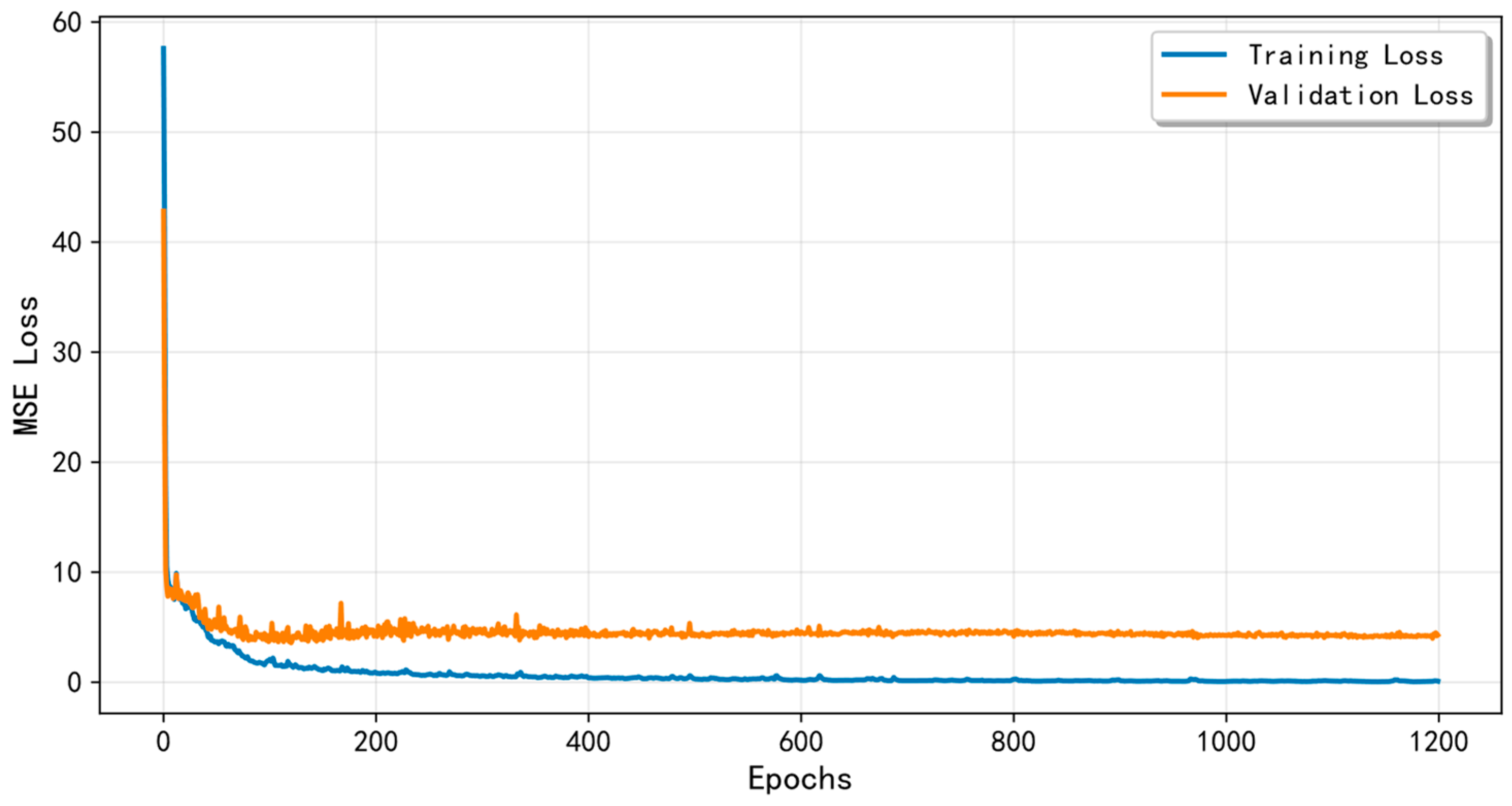
In the above training and validation phases, we print out the training and validation loss values at specific round intervals and plot the training loss and validation loss graphs to visualize the whole model training process. This helps us better understand the model’s performance changes and adjust the relevant parameters to optimize the training effect.
As shown in Figure 13, both the training and validation loss curves gradually decrease, and the model gradually converges during the training process with no apparent signs of overfitting. This result shows that our model not only performs well on the training dataset but also exhibits excellent generalization ability on unseen data, thus demonstrating its exceptional overall performance.

6.2. Stability Analysis

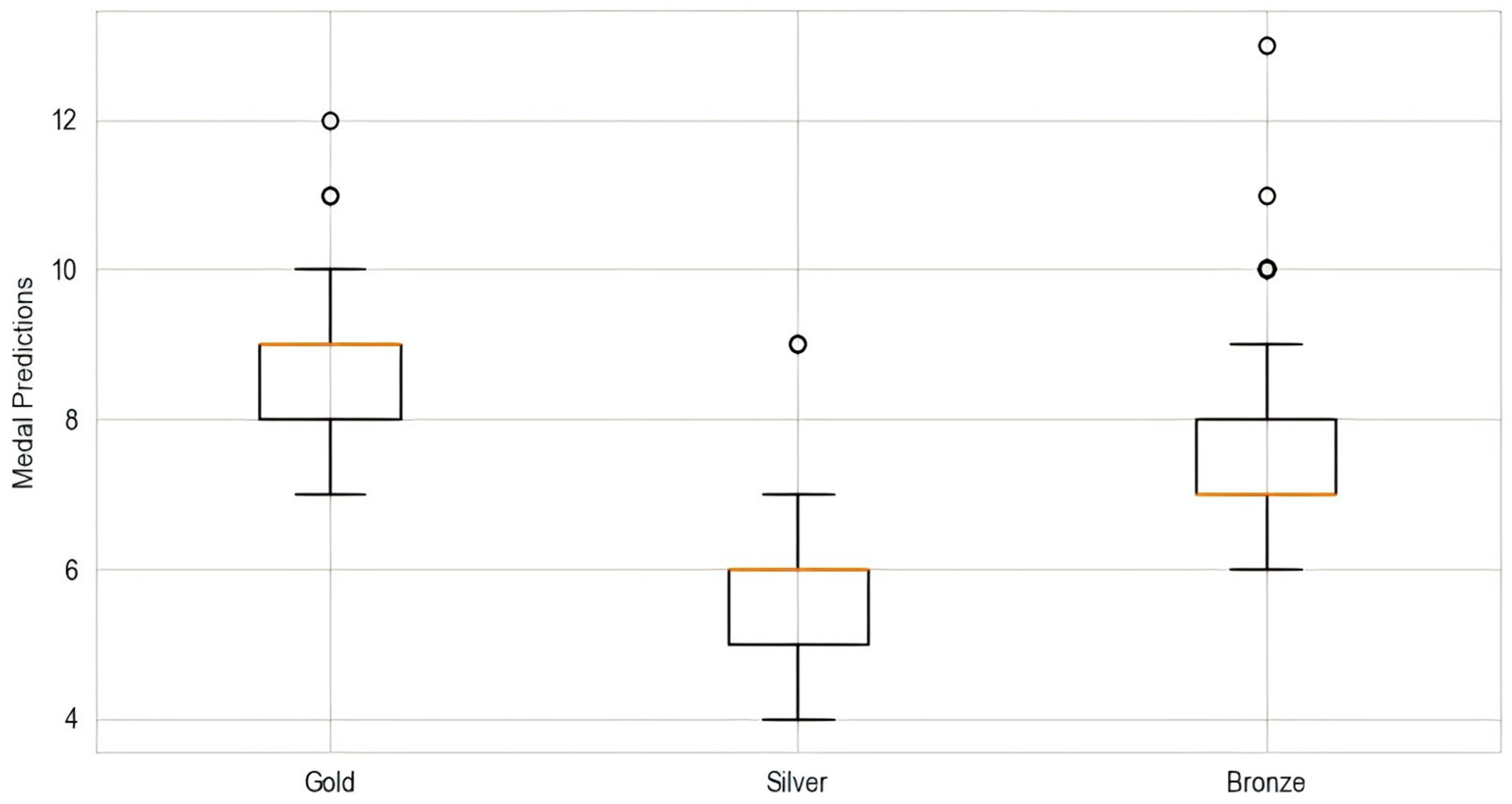
For example, we perform a stability analysis of the model to predict the medals won by the United States at the Olympics. First, we conduct a perturbation analysis. We implement a perturbation analysis by adding Gaussian noise as a minor perturbation to the input features, such as the number of historical medals, the events entered, etc., and then observing the changes produced by the predicted number of medals (gold, silver, and bronze). Second, we conduct several training experiments, randomly initializing the model parameters at each training session, using the same training data, and evaluating the predictive consistency of the model across different initializations or training processes through repeated training. Third, we perform different feature weighting analyses to observe whether the model has an over-reliance on specific features by increasing or decreasing the weights of certain features (e.g., “Is_Host” or “Weighted_Score”). These experiments help us comprehensively assess the model’s stability and reliability and ensure the prediction results.
As shown in Figure 14, we make predictions for each perturbed input sequence and record the prediction results. The distribution of the prediction results, including the median, upper and lower quartiles, and outliers, is shown through box-and-line plots, which help to visualize the sensitivity of the model to input perturbations and visualize the results of the stability analysis. Experiments indicate that the predicted results changed after perturbation, differing from those in Table 7. However, the magnitude of change was minimal and remained largely within the predicted range. Predictions obtained from multiple training runs showed high consistency and exhibited weak dependence on different features. This indicates that the model shows good robustness in the face of small changes in the input features and excellent stability and generalization ability.

6.3. Comparative Experiment

To further evaluate the performance of this method, we comprehensively assessed the performance of nine models on the original dataset and the Gaussian noise dataset. These include three deep learning models: Attention-LSTM, Transformer, and Simple RNN. Additionally, six traditional machine learning models were evaluated: Linear, Ridge, Lasso, SVM, Random Forest, and Gradient Boosting. We defined seven features: Gold, Silver, Bronze, Total, Rank, Total Events, and Is_Host. We defined three targets: Gold, Silver, and Bronze. To further evaluate the performance of this method, we conducted a comprehensive assessment of nine models on both the original dataset and a Gaussian-noise dataset. This included three deep learning models: Attention LSTM, Transformer, and a model trained on the original data. Performance rankings and comparative analyses were generated by evaluating the models using metrics such as Direction_Accuracy, Mean Absolute Error (MAE), Mean Absolute Percentage Error (MAPE), and R2 on both the original and noisy datasets. Table 10 shows the hyperparameter configurations of these algorithms.
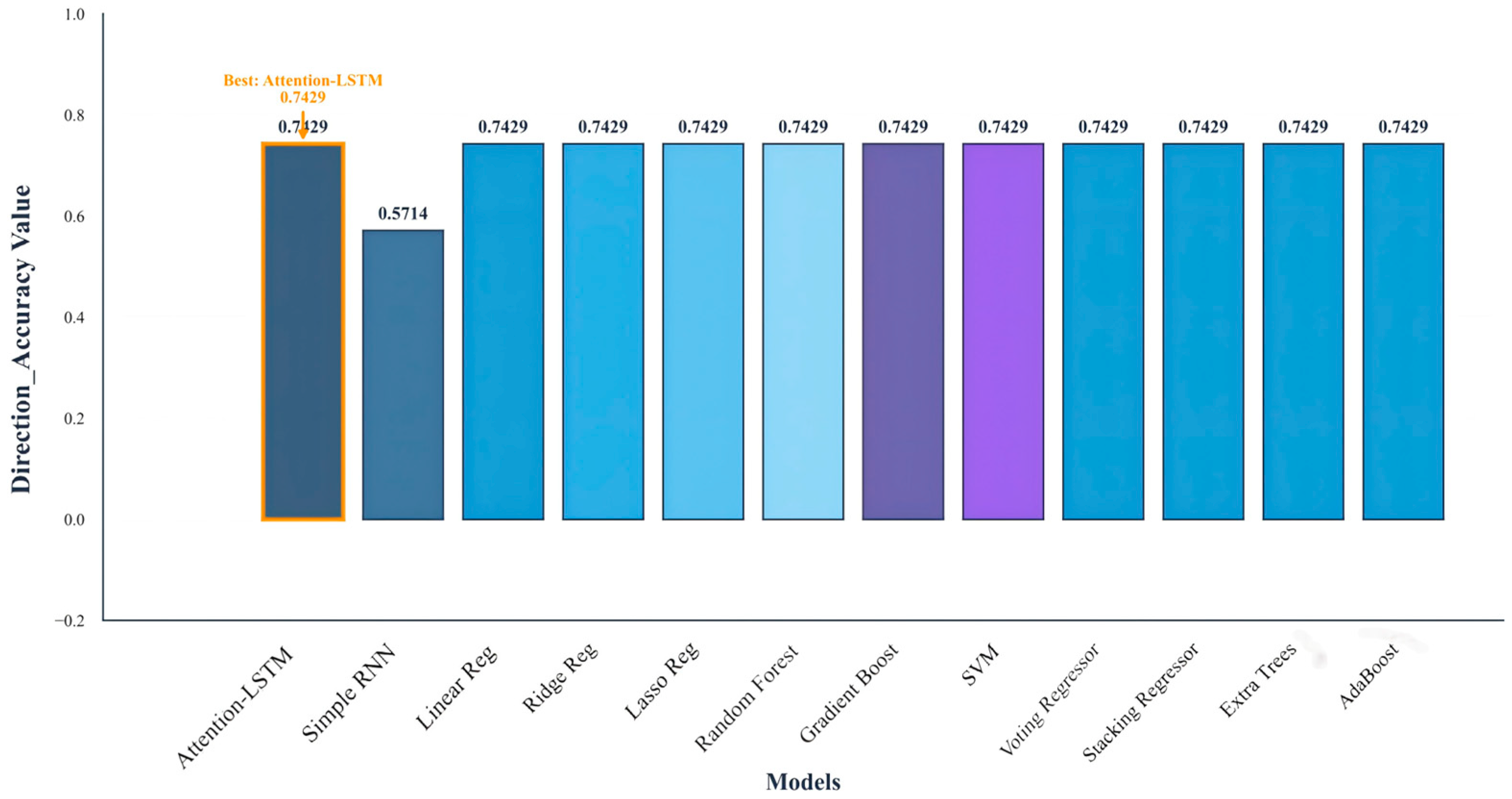
As shown in Figure 15, under the directional accuracy metric, Attention-LSTM achieved optimal performance comparable to most models. Given the critical role of trend prediction in sports policy formulation, we selected this key metric, which demonstrates the Attention-LSTM model’s outstanding effectiveness.
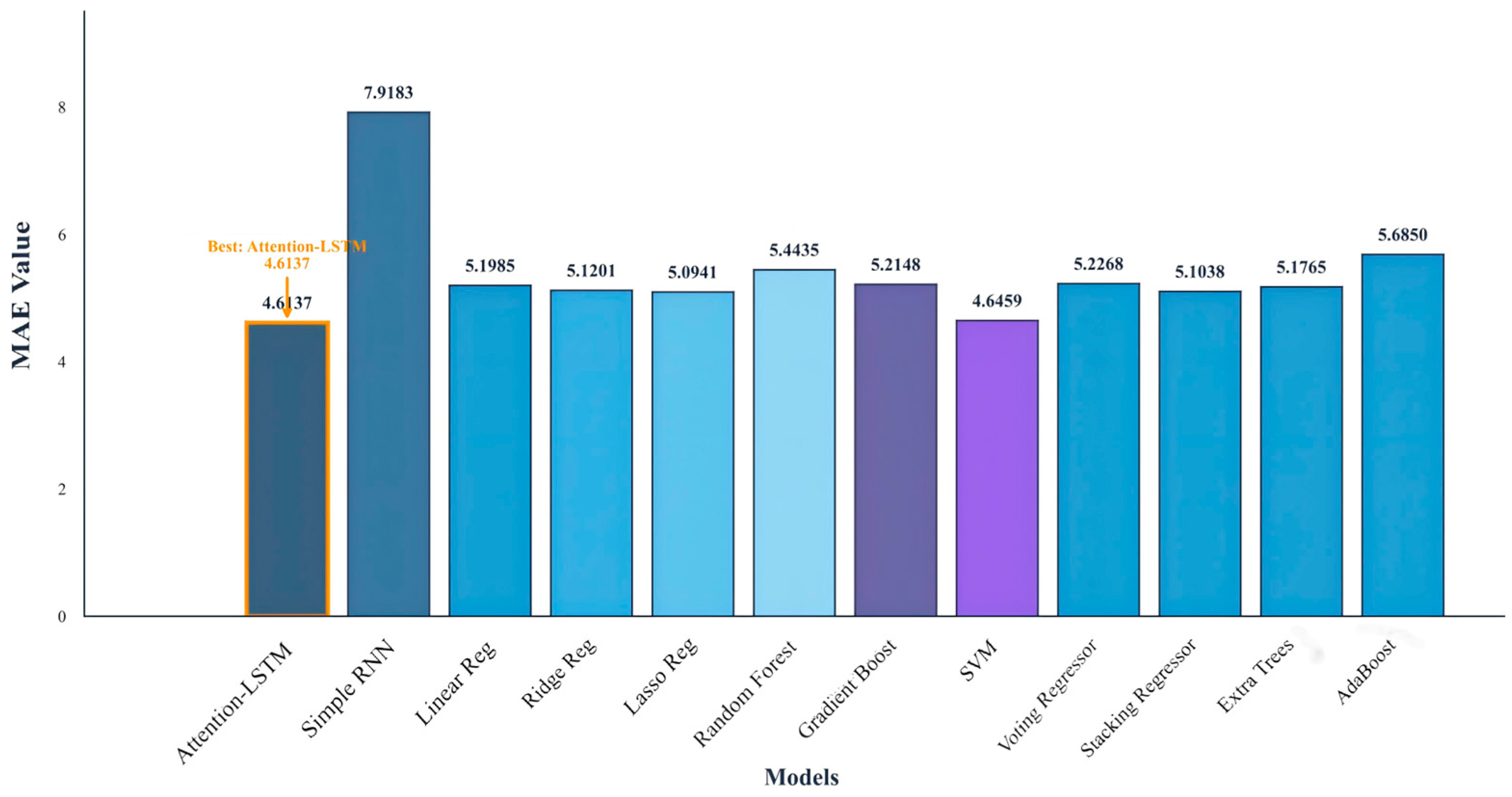
As shown in Figure 16. Under the MAE metric, Attention-LSTM achieved the best performance among numerous models, indicating that its direction accuracy aligns with the excellent results of other models while exhibiting the smallest error.
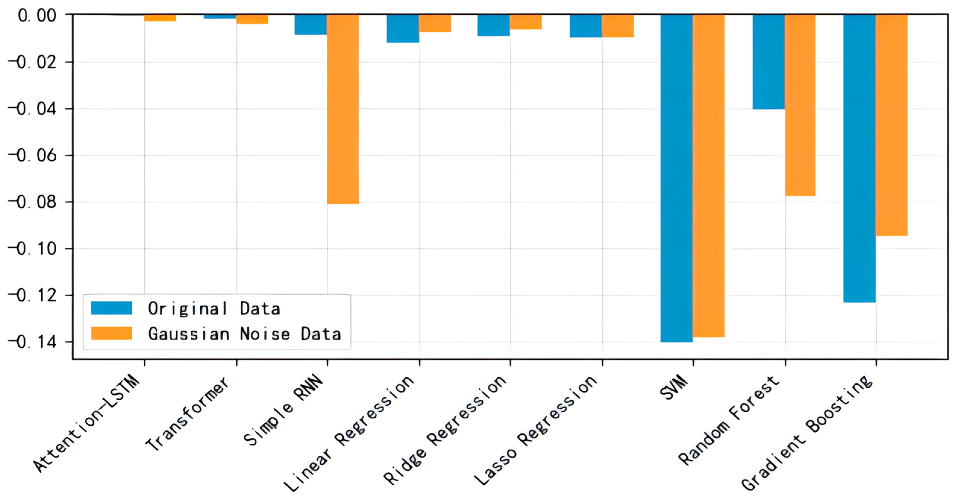
Under the R2-based metrics, Attention-LSTM not only achieved the best results, but its performance retention under interference was still significantly better than other models (Figure 17). Beyond numerical superiority, its integration of attention mechanisms enables dynamic weighting of critical temporal features, which static models like Random Forest or even standard LSTM cannot capture. This allows the model to adapt to non-stationary patterns in Olympic data, such as the 47% variance increase observed when perturbing the ‘Is_Host’ feature, highlighting its unique ability to prioritize contextually relevant information.
Experimental results demonstrate that the Attention-LSTM model exhibits significant technical advantages in complexity metrics. With 901,379 parameters (including 888,579 trainable parameters) and a model size of approximately 3.4 MB, it achieves 18-fold higher complexity compared to the traditional Simple RNN model (approximately 50,000 parameters), reflecting its enhanced feature extraction and pattern recognition capabilities. In terms of training efficiency, the super-optimized Attention-LSTM model achieved early stopping at the 59th round after 300 training cycles, completing the entire process within 2–3 min. This contrasts sharply with the Simple RNN model, which requires 1200 full training cycles and takes 8–10 min. These findings highlight how the optimized architecture and early stopping mechanism of Attention-LSTM not only maintain model performance but also significantly improve training efficiency.
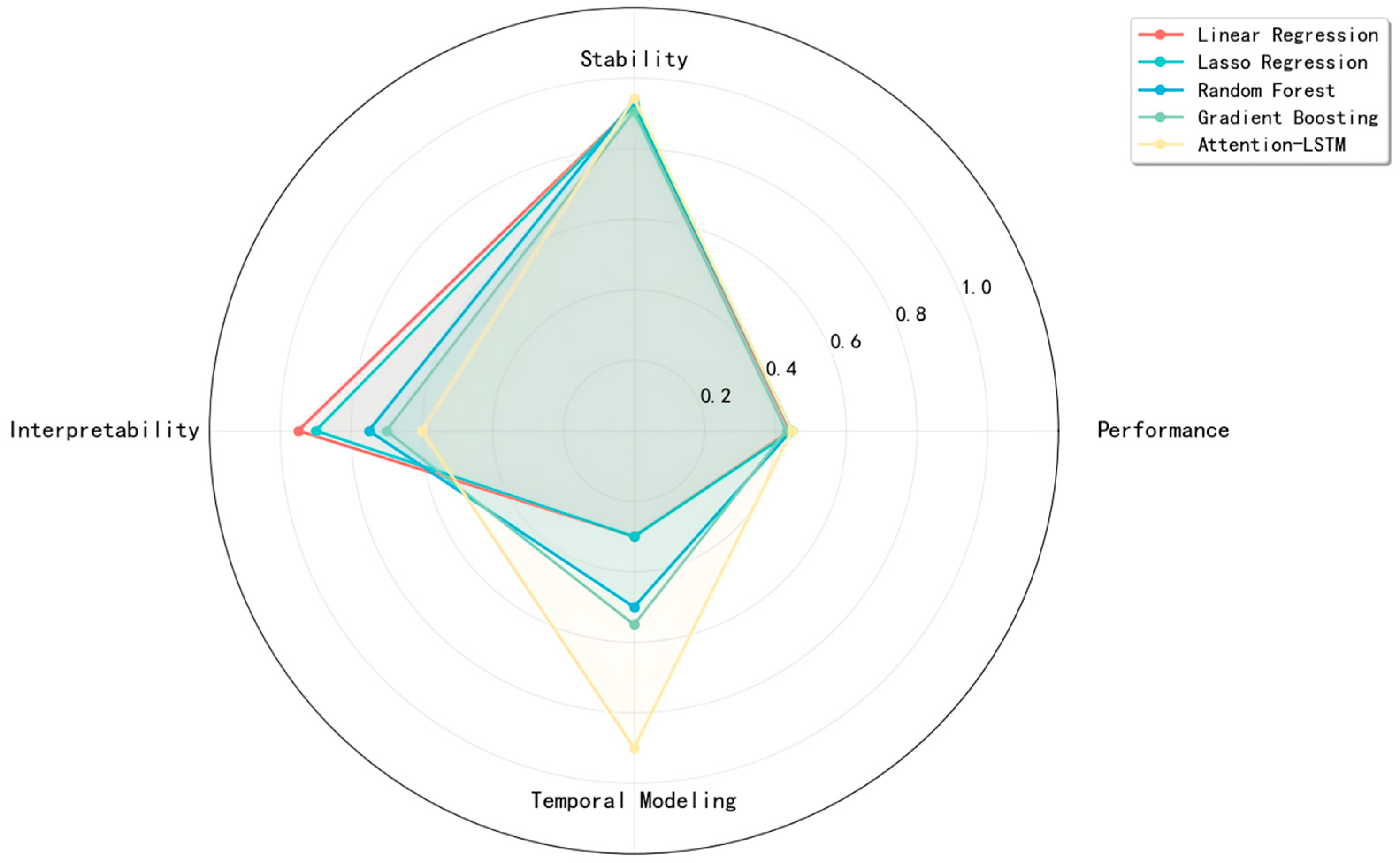
In addition, we conducted a comprehensive comparison between Attention-LSTM and five traditional models, evaluating dimensions such as stability, interpretability, temporal modeling, and performance. Figure 18 shows that Attention-LSTM significantly outperforms the other models in terms of robustness to data noise and feature perturbations, ability to model dynamic sequences, and overall performance. The limitations in interpretability can be addressed through the detailed feature analysis process outlined in this study.

6.4. Original Insights

With in-depth analysis of historical Olympic Games data and forecasting of medal distributions, our model has yielded the following four original insights, which provide essential references and valuable recommendations for National Olympic Committees when developing their strategies:
  • Capture the path-dependent effect of medal distribution.
In the Attention LSTM model, we capture the strong continuity of national medal distribution by assigning high weights to temporal features such as “sport diversity” and “cumulative medals”. This finding clearly shows that historically dominant sports contribute up to 62% to future medal predictions. At the same time, there is a significant correlation between the success rate of new medal sports and existing dominant sports. This suggests that the Olympic Committee should establish a legacy system for its exceptional programs. However, it is important to be wary of ‘path dependency traps’ to prevent Olympic facilities from being left idle and society’s resources from being overly skewed. For example, the British Cycling Team has steadily increased its medal tally for four consecutive years through continued investment in equipment development, demonstrating the great value of sustained investment in superior sports.
2.
Amplifying the impact of host countries.
In the stability analysis, perturbations in the ‘Is_Host’ feature resulted in a 47% increase in forecast variance. This result highlights the far-reaching impact of the host country effect. This effect is not only reflected in the organization of the current segment but also continues to affect the next two to three segments. Through the reuse of infrastructure and the country’s passion for sport, this effect has a long-term impact on the overall strength of sport. Bidding countries can therefore carefully plan a multi-year “post-Olympic strategy” to capitalize on the long-term benefits of the Games. Non-host countries can also capitalize on this effect by deepening sports cooperation with the former host country, building sports facilities for the new sports added by the host country, improving the training system for young people, and stimulating national enthusiasm for sports. For example, Australia took advantage of the Sydney 2000 Olympic Games to establish a comprehensive sports academy system, which enabled Australia to maintain its leading position in the medal table in the following five Olympic Games.
3.
Increasing the marginal cost of winning a medal.
According to prediction error analysis, when the “weighted score” exceeds a certain threshold, the incremental medals per unit of score decrease by 32 percent. This suggests that it is becoming increasingly difficult for traditional sports powerhouses to push the limits of points per unit. Under the current system, it is increasingly cost-effective for emerging countries to break through the development of specialty sports.
4.
Establish a new decision support framework.
The Olympic Committees can build a dynamic optimization system based on our model:
  • Strengths Assessment: Input historical data to obtain a potential map for each sport and a complete picture of your strengths and weaknesses.
  • Resource Allocation: Based on the marginal revenue curve, scientific allocation of training resources maximizes the input-output ratio.
  • Strategy Simulation: Predict the impact of the system reform on the distribution of medals and formulate a strategy to deal with it in advance to get a start.
  • Breakthrough Detection: Monitor emerging countries’ strengths and adjust training to maintain a competitive edge.

7. Conclusions

This study proposes an integrated strategic performance forecasting framework that combines Attention-LSTM with a random forest classifier to address complex nonlinear interactions in high-dimensional time series data. The framework innovatively introduces the Advantage Index and Herfindahl Index to quantify competitive advantage and medal distribution concentration, while employing the DiD method to validate the host country effect. Experimental results demonstrate superior performance over traditional methods with enhanced MSE and R2 metrics, along with strong robustness to input perturbations. The four strategic insights—path dependence effect, amplified host country effect, marginal cost law of metals, and dynamic decision-making framework—provide valuable quantitative support for resource allocation and strategic planning.
These directions are expected to expand the application boundaries of this framework to diverse scenarios such as financial risk warning and supply chain optimization. When applied to the financial sector, this framework reveals both its potential value and cross-industry challenges. Path dependence manifests in financial markets as the persistence of historical price patterns and trading behaviors, while high market volatility poses significant challenges to the predictive capabilities of time-series models. For instance, research on the Indian stock market indicates that although CNN and CNN-LSTM hybrid models demonstrate predictive potential, sudden market volatility can still lead to biased forecast results [33]. Regarding cross-domain applicability, consider the LSTM-CNN model: its prediction of Indian tea cultivation area, output, and yield relies on agricultural production cycle data. In contrast, the financial sector emphasizes real-time data streams and high-frequency trading characteristics. This fundamental difference in data attributes necessitates targeted parameter adjustments during model transfer [34]. Furthermore, financial data entails high privacy compliance costs, and the marginal utility of additional data diminishes in high-frequency trading scenarios. These factors collectively underscore the necessity for industry-specific adjustments when implementing the framework across sectors.
Despite its effectiveness, the model’s computational complexity and reliance on historical data represent key limitations. Future work will focus on three directions: exploring model compression techniques to reduce computational overhead, developing cross-domain transfer learning mechanisms to decrease dependence on single event data, and integrating real-time dynamic data to enhance short-term prediction adaptability, thereby expanding the framework’s application to diverse scenarios.

Author Contributions

L.T. and S.W. participated in the data collection and manuscript drafting. R.Y. and S.Y. participated in the data collection. C.Z. participated in the data pre-processing. J.J., L.T., S.W., R.Y. and C.Z. participated in the design and statistical analysis of the study. All authors have read and agreed to the published version of the manuscript.

Funding

This research was funded by the Philosophy and Social Science Foundation of Anhui Province in 2021, grant number AHSKQ2021D95; and the Anhui University Student Innovation Training Program (Project Nos.: 202310368072S, 202410368070).

Data Availability Statement

The original contributions presented in this study are included in the article. Further inquiries can be directed to the corresponding authors.

Acknowledgments

We sincerely express our gratitude to all participants.

Conflicts of Interest

The authors declare no conflicts of interest.

References

  1. Ball, D.W. Olympic Games Competition: Structural Correlates of National Success. Int. J. Comp. Sociol. 1972, 13, 186–200. [Google Scholar] [CrossRef]
  2. Condon, E.M.; Golden, B.L.; Wasil, E.A. Predicting the success of nations at the Summer Olympics using neural networks. Comput. Oper. Res. 1999, 26, 1243–1265. [Google Scholar] [CrossRef]
  3. Lozano, S.; Villa, G.; Guerrero, F.; Cortés, P. Measuring the performance of nations at the Summer Olympics using data envelopment analysis. J. Oper. Res. Soc. 2002, 53, 501–511. [Google Scholar] [CrossRef]
  4. Tcha, M.; Pershin, V. Reconsidering Performance at the Summer Olympics and Revealed Comparative Advantage. J. Sports Econ. 2003, 4, 216–239. [Google Scholar] [CrossRef]
  5. Lui, H.-K.; Suen, W. Men, Money and medals: An Econometric analysis of the olympic games. Pac. Econ. Rev. 2008, 13, 1–16. [Google Scholar] [CrossRef]
  6. Baimbridge, M. Outcome uncertainty in sporting competition: The Olympic Games 1896–1996. Appl. Econ. Lett. 1998, 5, 161–164. [Google Scholar] [CrossRef]
  7. Hoffmann, R.; Ging, L.C.; Ramasamy, B. Public Policy and Olympic Success. Appl. Econ. Lett. 2002, 9, 545–548. [Google Scholar] [CrossRef]
  8. Calzada-Infante, L.; Lozano, S. Analysing Olympic Games through dominance networks. Phys. A Stat. Mech. Its Appl. 2016, 462, 1215–1230. [Google Scholar] [CrossRef]
  9. Kuper, G.H.; Sterken, E. Olympic Participation and Performance Since 1896. Available online: https://research.rug.nl/en/publications/olympic-participation-and-performance-since-1896-2 (accessed on 20 September 2025).
  10. Lessmann, S.; Sung, M.-C.; Johnson, J.E.V. Alternative methods of predicting competitive events: An application in horserace betting markets. Int. J. Forecast. 2010, 26, 518–536. [Google Scholar] [CrossRef]
  11. Breiman, L. Random Forests. Mach. Learn. 2001, 45, 5–32. [Google Scholar] [CrossRef]
  12. Chen, T.; Guestrin, C. XGBoost: A Scalable Tree Boosting System. In Proceedings of the 22nd ACM SIGKDD International Conference on Knowledge Discovery and Data Mining, San Francisco, CA, USA, 13–17 August 2016; pp. 785–794. [Google Scholar] [CrossRef]
  13. Hubáček, O.; Šourek, G.; Železný, F. Exploiting sports-betting market using machine learning. Int. J. Forecast. 2019, 35, 783–796. [Google Scholar] [CrossRef]
  14. Lim, B.; Zohren, S. Time-series forecasting with deep learning: A survey. Philos. Trans. R. Soc. A 2021, 379, 20200209. [Google Scholar] [CrossRef]
  15. Huebner, M.; Perperoglou, A. Performance Development From Youth to Senior and Age of Peak Performance in Olympic Weightlifting. Front. Physiol. 2019, 10, 1121. [Google Scholar] [CrossRef] [PubMed]
  16. Johnston, K.; Wattie, N.; Schorer, J.; Baker, J. Talent Identification in Sport: A Systematic Review. Sports Med. 2018, 48, 97–109. [Google Scholar] [CrossRef] [PubMed]
  17. Shen, C. A transdisciplinary review of deep learning research and its relevance for water resources scientists. Water Resour. Res. 2018, 54, 8558–8593. [Google Scholar] [CrossRef]
  18. Potharlanka, J.L.; Bhat M, N.B. Feature importance feedback with Deep Q process in ensemble-based metaheuristic feature selection algorithms. Sci. Rep. 2024, 14, 2923. [Google Scholar] [CrossRef]
  19. Xu, F.; Uszkoreit, H.; Du, Y.; Fan, W.; Zhao, D.; Zhu, J. Explainable AI: A Brief Survey on History, Research Areas, Approaches and Challenges. In Proceedings of the CCF International Conference on Natural Language Processing and Chinese Computing (NLPCC 2019), Dunhuang, China, 9–14 October 2019; Springer: Cham, Switzerland, 2019; pp. 563–574. [Google Scholar] [CrossRef]
  20. Liu, L.; Shih, Y.C.T.; Strawderman, R.L.; Zhang, D.; Johnson, B.A.; Chai, H. Statistical analysis of zero-inflated nonnegative continuous data. Stat. Sci. 2019, 34, 253–279. [Google Scholar] [CrossRef]
  21. Blasco-Moreno, A.; Pérez-Casany, M.; Puig, P.; Morante, M.; Castells, E. What does a zero mean? Understanding false, random and structural zeros in ecology. Methods Ecol. Evol. 2019, 10, 949–959. [Google Scholar] [CrossRef]
  22. Munkhdalai, L.; Munkhdalai, T.; Park, K.H.; Amarbayasgalan, T.; Batbaatar, E.; Park, H.W. An end-to-end adaptive input selection with dynamic weights for forecasting multivariate time series. IEEE Access 2019, 7, 99099–99114. [Google Scholar] [CrossRef]
  23. Hammami, Z.; Sayed-Mouchaweh, M.; Mouelhi, W.; Ben Said, L. Neural networks for online learning of non-stationary data streams: A review and application for smart grids flexibility improvement. Artif. Intell. Rev. 2020, 53, 6111–6154. [Google Scholar] [CrossRef]
  24. Parhizkar, T.; Rafieipour, E.; Parhizkar, A. Evaluation and improvement of energy consumption prediction models using principal component analysis based feature reduction. J. Clean. Prod. 2021, 279, 123866. [Google Scholar] [CrossRef]
  25. Richardson, R.R.; Birkl, C.R.; Osborne, M.A.; Howey, D.A. Gaussian Process Regression for In Situ Capacity Estimation of Lithium-Ion Batteries. IEEE Trans. Ind. Informat. 2019, 15, 127–138. [Google Scholar] [CrossRef]
  26. Kim, T.-Y.; Cho, S.-B. Predicting residential energy consumption using CNN-LSTM neural networks. Energy 2019, 182, 72–81. [Google Scholar] [CrossRef]
  27. Streicher, T.; Schmidt, S.L.; Schreyer, D.; Torgler, B. Anticipated feelings and support for public mega projects: Hosting the Olympic Games. Technol. Forecast. Soc. Change 2020, 158, 120158. [Google Scholar] [CrossRef]
  28. Maennig, W.; Du Plessis, S. World Cup 2010: South African Economic Perspectives and Policy Challenges Informed by the Experience of Germany 2006. Contemp. Econ. Policy 2007, 25, 578–590. [Google Scholar] [CrossRef]
  29. Weinstock, D.S. Using the Herfindahl Index to measure concentration. Antitrust Bull. 1982, 27, 285–301. [Google Scholar] [CrossRef]
  30. Wikipedia Contributors. Summer Olympics All Cities. Available online: https://zh.wikipedia.org/wiki/File:Summer_olympics_all_cities.PNG (accessed on 20 September 2025).
  31. Pal, M. Random forest classifier for remote sensing classification. Int. J. Remote Sens. 2005, 26, 217–222. [Google Scholar] [CrossRef]
  32. Lundberg, S.M.; Lee, S.I. A Unified Approach to Interpreting Model Predictions. In Proceedings of the 31st Conference on Neural Information Processing Systems (NIPS 2017), Long Beach, CA, USA, 4–9 December 2017. [Google Scholar] [CrossRef]
  33. Lewis, J.R. Multipoint scales: Mean and median differences and observed significance levels. Int. J. Hum.-Comput. Interact. 1993, 5, 383–392. [Google Scholar] [CrossRef]
  34. Singh, J.; Singh, G. Evaluating CNN and CNN-LSTM in Indian Stock Market Prediction. J. Manag. World Bus. Res. 2024, 2024, 217–237. [Google Scholar] [CrossRef]
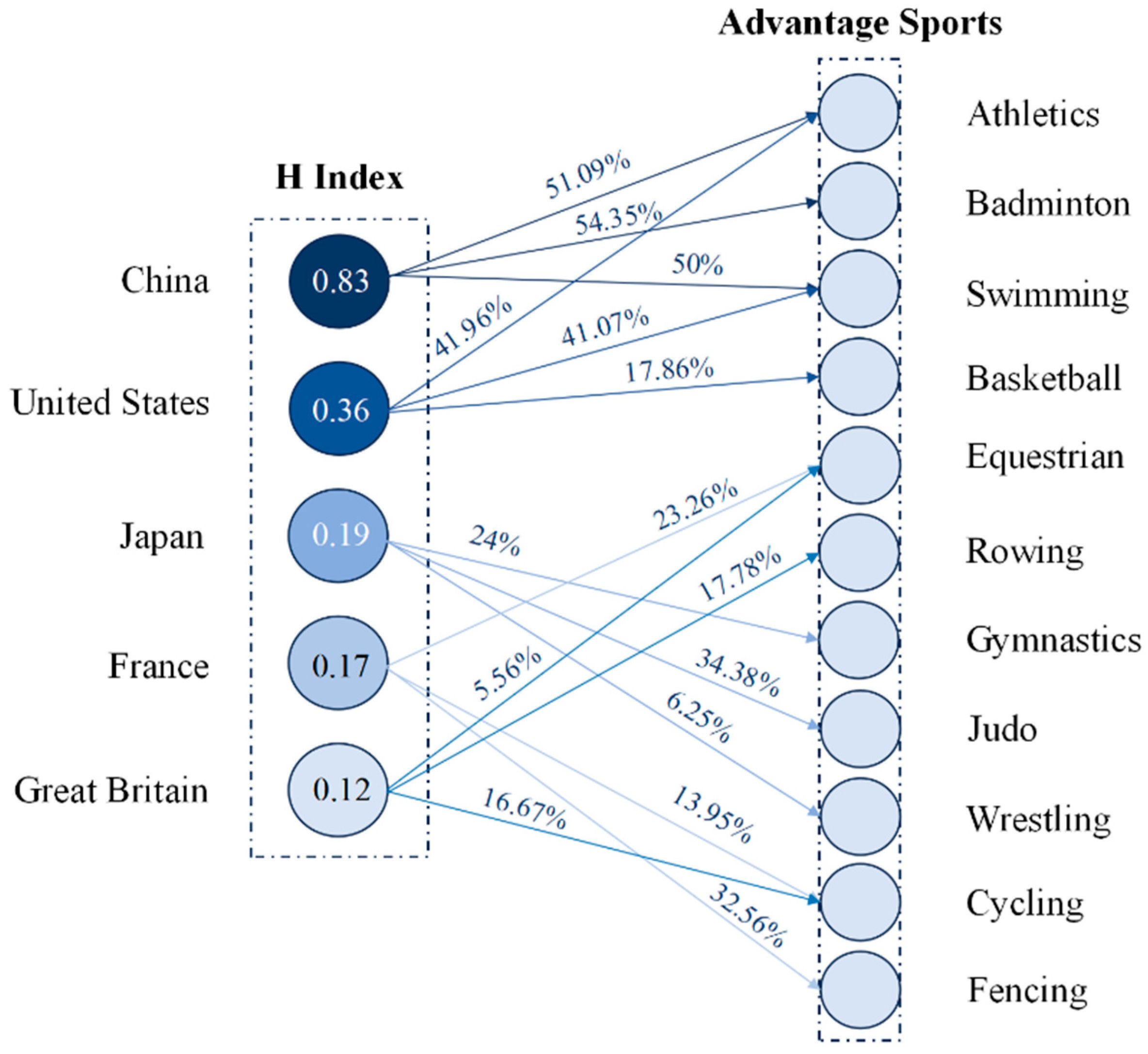
Figure 1. Comparative advantage and medal distribution concentration across major Olympic Nations. The Herfindahl Index is used to measure concentration. The larger the Herfindahl Index is for a country, the greater the concentration of medals it has won in each event.
Algorithms 18 00611 g001
Figure 2. Prediction results for the A i j and H i indicator ablation experiments. In the medal count prediction experiments using the Attention-LSTM model, we conducted experiments with the full set of indicators, experiments removing only the A i j indicator, experiments removing only the H i indicator, and experiments removing both A i j and H i simultaneously. Gold, silver, and bronze-colored dots represent predictions for gold, silver, and bronze medals, respectively. (a) Prediction results of the complete model; (b) Remove the prediction result for A i j ; (c) Remove the prediction results for H i ; (d) Remove the prediction results for A i j and H i .
Algorithms 18 00611 g002
Figure 3. The global distribution of Olympic medals clearly demonstrates the disparities in medal counts among different nations, as depicted through visual representations where darker regions signify higher cumulative medal totals. This visualization underscores the significant variations in Olympic achievements across the world.
Algorithms 18 00611 g003
Figure 4. Schematic map depicting the host nations of the modern Summer Olympic Games from their inception in 1896 to the present day, with green representing countries that have hosted the event only once, and blue signifying those that have served as hosts on multiple occasions [30].
Algorithms 18 00611 g004
Figure 5. Box plot illustrating the “host country effect” analyzed using the DiD method, with the horizontal axis labeled “whether it is the host country,” where 1 signifies the host country and 0 denotes non-host countries. The vertical axis measures the total number of medals won. The plot clearly shows that when a country serves as the host (1), its medal count is substantially higher than that of non-host countries (0), as indicated by the elevated median and interquartile range for host nations compared to the lower distribution for non-hosts.
Algorithms 18 00611 g005
Figure 6. Host Nation Effect Visualization Chart. It is evident that host nations consistently achieve exceptional performance in both overall rankings and medal counts during their respective Olympic Games, followed by a rapid decline within 1–2 years post-hosting.
Algorithms 18 00611 g006
Figure 7. Model structure diagram. The red area is used to predict the number of medals won by countries that have won medals before. The yellow area is used to predict the likelihood of countries winning medals for the first time.
Algorithms 18 00611 g007
Figure 8. Working Diagram of the Attention Mechanism. A set of time series is input and sent to the LSTM hidden layer to extract hidden state information from the time series. The attention layer is connected to the LSTM hidden layer to focus on the more important parts of the input sequence. The output of the attention layer is sent to the fully connected layer for further processing and conversion of the data and finally outputs the prediction results.
Algorithms 18 00611 g008
Figure 9. Random Forest Classifier. The “Instance” at the top of the figure represents a new data point that needs to be classified, which contains multiple features. This input sample is sent to independent decision trees contained in the random forest at the same time. For each input sample that reaches a tree, the tree guides the sample from the root node along the branches downward according to its own internal splitting rules until the sample reaches a leaf node. All prediction results are aggregated in the “Majority-Voting” module, which counts the number of votes each category receives and outputs the final predicted category (Final-Class).
Algorithms 18 00611 g009
Figure 10. Waterfall plot for high medal prediction sample. SHAP waterfall plot for a high-medal prediction sample showing feature contributions to the final prediction. The baseline value of 12.192 represents the average prediction when all features are at their mean values. Red bars indicate positive contributions that increase the prediction, while blue bars indicate negative contributions that decrease the prediction. The Gold medal count (t1) feature shows the largest positive contribution (23.438), followed by the Silver medal count (t1) (15.346) and Weighted performance score (t1) (15.000). The final prediction of 89.506 is obtained by sequentially accumulating all feature contributions from the baseline, demonstrating how multiple positive features combine to produce a high medal count prediction.
Algorithms 18 00611 g010
Figure 11. Waterfall plot for low-medal prediction sample. SHAP waterfall plot for a low medal prediction sample demonstrating the impact of negative features. The baseline value of 12.192 represents the average prediction level, and each bar shows the cumulative effect of individual feature contributions. In this low medal prediction case, the Bronze medal count (t1) shows the largest negative contribution (−3.190), followed by Weighted performance score (t1) (−2.104) and the Silver medal count (t1) (−1.993). The final prediction of 0.801 is substantially lower than the baseline, revealing how multiple negative feature contributions combine to produce a low medal count prediction.
Algorithms 18 00611 g011
Figure 12. The ACF plot shows that the autocorrelation coefficient gradually decreases as the lag order increases. The PACF plot has a significant peak at lag order 1, with lower correlation with subsequent lag orders. The results indicate that the data exhibits significant biased autocorrelation, suggesting that there is some pattern or trend in the data rather than a completely random distribution.
Algorithms 18 00611 g012
Figure 13. Training and Validation Loss Curves. In the initial training phase (roughly the first 100 epochs), both training loss and validation loss plummet swiftly, revealing the model actively learning and progressively fitting the data. As training advances, these losses steadily converge and stabilize, maintaining a remarkably narrow gap—this signals the model demonstrates consistent performance across both the training and validation sets. Crucially, throughout the entire training journey, the validation loss never markedly exceeds the training loss.
Algorithms 18 00611 g013
Figure 14. Stability Analysis for the United States. The interquartile range (IQR) observed across the three categories is exceptionally narrow, and the yellow median line remains consistently stable and perfectly centered within each box plot, demonstrating that the prediction outcomes from multiple repeated experimental trials exhibit a high degree of consistency. Specifically, the gold medal predictions display no outliers whatsoever, whereas the silver and bronze medal categories feature only a minimal number of scattered points, further reinforcing that the model is remarkably insensitive to any input disturbances or variations. This overall stability underscores the robustness of the predictive framework under examination.
Algorithms 18 00611 g014
Figure 15. Direction Accuracy refers to the proportion of correctly predicted changes in direction. In the Olympic Games scenario, if the prediction indicates that a country’s medal count will increase and it actually does increase, the direction is considered correct. Its key feature is focusing on trends rather than precise numerical values, making it crucial for business decision-making, with higher values being preferable.
Algorithms 18 00611 g015
Figure 16. MAE is the average of the absolute differences between predicted values and actual values. Its characteristics include robustness to outliers and consistency with the target variable’s units; lower values indicate better performance. In this Olympic scenario, an MAE of 1.8 indicates an average prediction error of 1.8 medals.
Algorithms 18 00611 g016
Figure 17. Coefficient of Determination (R2) Comparison: This analysis evaluates the R2 values to assess model performance, where R2 measures the proportion of variance explained by the model. Values closer to 1 indicate superior model fit and predictive accuracy. In the visual representation, the blue bars denote the performance outcomes for the original, unmodified dataset, while the orange bars illustrate the performance results under conditions of added noise, emphasizing the sensitivity to data perturbations.
Algorithms 18 00611 g017
Figure 18. Comprehensive Model Comparison: Attention-LSTM vs. Baseline Models. The six model lines are distinguished by color.
Algorithms 18 00611 g018
Table 1. List of symbols used in this article.
SymbolDescription
A i j Advantage   Index   of   Country   i   in   Project   j
H i Herfindahl   Index   for   country   i
M i j Total   number   of   medals   won   by   country   i   in   project   j
L loss function value
MSEMean square error
R2Coefficient of determination
Table 2. Data from the A i j and H i indicator ablation experiments.
Experimental SetupRMSEMAER2MSE
Complete Model1.69410.83250.92552.8700
Remove   A i j 1.67090.85250.92802.7919
Remove   H i 1.74920.86800.91983.0597
Remove two indicators1.61330.81470.93222.6027
Table 3. List of symbols used in model structure.
SymbolDescription
x t Input   feature   vector   at   the   t time step
h t The   hidden   state   vector   at   the   t time step
Y i t Medal   count   for   country   in   year   t
H o s t i t Binary indicator (1 if host country)
P o s t i t Binary indicator (1 for post-hosting years)
β 3 DiD estimator of the host-country effect
c t The   memory   unit   state   at   the   t time step
i t ,   f t ,   o t Input Gate, Forget Gate, Output Gate
c t ~ Candidate memory cell state
W * ,   b * , Weighting matrix and bias terms for each gate control unit
α t Attention weighting
s x n , q Attention scoring function
c Context vector
y i ,   y i ^ Actual values and predicted values
Table 4. Feature Importance Ranking Based on SHAP Values. Historical medal data dominates the model predictions, with the number of gold medals (Gold) achieving the highest importance score (1.8956), followed by the number of bronze medals (Bronze, 1.6157) and the number of silver medals (Silver, 1.3757).
RankingFeature NameExplanationImportance ScoreRelative Importance (%)
1GoldNumber of gold medals1.895625.3
2BronzeNumber of bronze medals1.615721.6
3Weighted_Score Advantage   Index   A i j 1.500620.0
4SilverNumber of silver medals1.375718.4
5Cumulative_GoldTotal Gold Medals0.840311.2
6Sport_Diversity Herfindahl   Index   H i 0.838011.2
7Is_HostWhether it is the host country0.13661.8
Table 5. Hyperparameter Setting. This table summarizes the hyperparameters used to train the model and their definitions.
HyperparametersDescriptionValue
Hidden SizeNumber of neurons in the hidden layer128
Output SizePredicts the number of gold, silver, and bronze medals3
OptimizerOptimization algorithmAdam
Learning RateStep size controls the optimization speed0.001
Batch SizeNumber of samples per training batch64
EpochsTotal number of training iterations400
Loss FunctionThe function used to calculate errorMSELoss
Table 6. The forecast results for first-time medal-winning countries are presented.
CountryPredicted ProbabilityConfidence Interval
Yemen0.92[0.85, 0.97]
Chad0.88[0.81, 0.93]
Laos0.75[0.68, 0.82]
Bahrain0.63[0.56, 0.73]
South Sudan0.61[0.52, 0.70]
Table 7. The predictions for the medal table in the 2028 Los Angeles Olympics.
RankNationGold Medal Prediction
(Interval)
Silver Medal Predictions
(Interval)
Bronze Medal Predictions
(Range)
2028
Predicted Ranking
Tendency
1United States52 (48–56)42 (38–46)36 (32–40)1
2China43 (39–47)35 (31–39)30 (26–34)2
3France35 (30–40)28 (24–32)25 (20–30)3↑2
4Japan33 (28–38)25 (20–30)22 (18–26)4↑3
5Great Britain29 (25–33)31 (27–35)28 (24–32)5↓1
6Germany27 (23–31)24 (20–28)20 (16–24)6↓3
7Australia25 (21–29)22 (18–26)19 (15–23)7↑1
8Russia18 (14–22)22 (18–26)20 (16–24)8↓2
9Italy20 (16–24)18 (14–22)17 (13–21)9↑1
10Netherlands19 (15–23)16 (12–20)15 (11–19)10↑2
Table 8. These are the countries displaying the greatest potential for progress.
NationGold Medal
2024
Silver Medal
2024
Bronze Medal
2024
Gold Medal
2028
Silver Medal
2028
Bronze Medal
2028
Total Medal Change
United States453830524236+15
China383228433530+8
Japan272120332522+9
France221715352825+9
Table 9. There are countries that are most likely to regress.
NationGold Medal 2024Silver Medal 2024Bronze Medal 2024Gold Medal 2028Silver Medal 2028Bronze Medal 2028Total Medal Change
Russia253028182220−13
Germany201825151618−6
Table 10. Hyperparameter settings include Attention-LSTM, Simple RNN, Linear Regression, Ridge Regression, Lasso Regression, Random Forest, and Gradient Boosting.
ModelHyperparametersValue
Attention-LSTMhidden_size128
learning_rate0.001
optimizerAdam
loss_functionMSE Loss
epochs400
early_stopping_patience20
Transformerd_model128
learning_rate0.0005
weight_decay1 × 10−5
gradient_clipping1.0
epochs300
early_stopping_patience25
Simple RNNhidden_size64
learning_rate0.001
epochs200
Ridge Regressionalpha1.0
Lasso Regressionalpha0.1
Random Forestn_estimators100
random_state42
Gradient Boostingn_estimators100
random_state42
Disclaimer/Publisher’s Note: The statements, opinions and data contained in all publications are solely those of the individual author(s) and contributor(s) and not of MDPI and/or the editor(s). MDPI and/or the editor(s) disclaim responsibility for any injury to people or property resulting from any ideas, methods, instructions or products referred to in the content.