Article

Backward Signal Propagation: A Symmetry-Based Training Method for Neural Networks

School of Electrical Engineering, Chongqing University, Chongqing 400044, China
*
Author to whom correspondence should be addressed.
Algorithms 2025, 18(10), 594; https://doi.org/10.3390/a18100594
Submission received: 4 August 2025 / Revised: 4 September 2025 / Accepted: 22 September 2025 / Published: 23 September 2025

Abstract

While backpropagation (BP) has long served as the cornerstone of training deep neural networks, it relies heavily on strict differentiation logic and global gradient information, lacking biological plausibility. In this paper, we systematically present a novel neural network training paradigm that depends solely on signal propagation, which we term Backward Signal Propagation (BSP). The core idea of this framework is to reinterpret network training as a symmetry-driven process of discovering inverse causal relationships. Starting from symmetry principles, we define symmetric differential equations and leverage their inherent properties to implement a learning mechanism analogous to differentiation. Furthermore, we introduce the concept of causal distance, a core invariant that bridges the forward propagation and inverse learning processes. It quantifies the influence strength between any two elements in the network, leading to a generalized form of the chain rule. With these innovations, we achieve precise, pointwise adjustment of model parameters. Unlike traditional BP, the BSP method enables parameter updates based solely on local signal features. This work offers a new direction toward efficient and biologically plausible learning algorithms.

1. Introduction

1.1. Backpropagation Algorithm

Training has always been a central issue in the development of neural networks. Throughout the various surges and declines in the history of artificial neural networks, the evolution of training methods has played a pivotal role in determining the success or stagnation of the field [1,2].
Since the 1980s, the emergence of the backpropagation (BP) algorithm has removed the primary obstacle in neural network training, granting artificial neural networks theoretically unlimited potential [3]. Remaining engineering challenges—such as vanishing and exploding gradients [4], insufficient training data [5], and computational inefficiencies [6]—have been addressed progressively through sustained research efforts.
Today, the backpropagation algorithm holds a dominant position in neural network training, primarily due to its ability to perform pointwise precise parameter updates. For any given parameter, BP provides an explicit relationship to the final error, enabling highly efficient optimization of neural networks [7].
Moreover, a family of optimization methods built upon backpropagation—such as stochastic gradient descent (SGD) and adaptive moment estimation (Adam) [8,9]—has greatly extended the applicability of BP, providing robust support for training neural networks of various architectures.

1.2. The Core Contradiction of the Backpropagation Algorithm

Despite its unparalleled success, the backpropagation algorithm has long been the subject of skepticism among researchers [10,11]. The core issue preventing the replacement of BP lies in the absence of an alternative mechanism that can efficiently track inverse causal relationships during training.
The fundamental strength of BP lies in two key techniques: differentiation and the chain rule of propagation [7]. Differentiation enables the analysis of causal relationships between any two variables in an equation, while the chain rule reflects the topological structure of the network [3]. The combination of these two allows BP to systematically infer how each parameter contributes to the final error across arbitrarily complex architectures. This capacity for tracing inverse causality makes it possible to perform precise error-driven adjustments for any parameter in the network.
However, the very foundations of BP also raise two major concerns regarding biological plausibility:
  • Differentiation in biological neurons: It remains unclear whether biological neurons are capable of performing differentiation. Modern artificial neural networks employ a wide variety of activation functions, each designed to be differentiable. Yet, such mathematical operations—and the diverse function types themselves—appear to have no biological counterpart [12].
  • Global error propagation: The chain rule in BP assumes that error signals can be propagated globally across the network, requiring each neuron to possess a form of global awareness to compute gradients based on upstream signals. This assumption, however, is biologically unrealistic, as real neurons operate primarily on local information and lack such global processing capability [13].
These two issues lie at the heart of the debate over the biological plausibility of BP. Despite ongoing criticism, the algorithm remains a cornerstone of modern neural network training.
In order to solve the core contradiction of the backpropagation algorithm, people have never given up research on biological nerve cells. On the one hand, biological nerve cells have natural biological rationality. On the other hand, biological neural networks also have higher energy utilization efficiency. For example, the human brain only needs very low power to achieve efficient logical reasoning and mathematical calculations.

1.3. Inspiration from Differential Geometry

We argue that the key to overcoming the current predicament lies in moving beyond the reliance on a “global perspective” and reconstructing the computation and learning processes of neural networks upon a local and continuous framework. This shift in conceptual paradigm does not emerge in a vacuum; rather, its most important inspiration stems from the historical emergence and evolution of differential geometry in the history of mathematics. The development of differential geometry itself constitutes a grand narrative—a transition from the study of rigid, global shapes to the analysis of flexible, local properties, ultimately integrating local information to comprehend complex global structures.
Before the advent of differential geometry, Euclidean geometry dominated the understanding of space. It dealt with global, rigid objects such as perfect straight lines, circles, and polyhedra. Its axiomatic approach was ill-suited to handle the ubiquitous curved, smooth, and deformable shapes found in the real world. This bears a striking resemblance to the situation of backpropagation: it operates flawlessly on an idealized, globally connected computational graph, yet struggles to adapt to more complex, dynamic, and resource-constrained physical realities.
The true transformation began with the invention of calculus in the 17th century, which provided researchers with a powerful tool to “infinitely zoom in” and examine local properties. Mathematicians began using derivatives and integrals to analyze the behavior of curves and surfaces within infinitesimal neighborhoods around each point, rigorously defining key concepts such as curvature and torsion. This marked the first leap in thinking: a shift from focusing on global shapes to concentrating on local characteristics. This offers us an insight: perhaps we, too, should temporarily set aside the global pursuit of the “optimal solution” for the entire network and instead investigate how neurons or neural assemblies can respond most efficiently and rationally based on the local signals they receive.

1.4. Solutions Based on Symmetric Differential Equations

To design a local system with desirable properties, we turned to group theory and, in combination with differential equations, constructed symmetric differential equations [14]. Owing to the inherent symmetry of group theory, these symmetric differential equations are reversible. By connecting multiple such symmetric differential equation systems, we formed a symmetric differential neural network. The reversibility of the system allows signals to propagate forward with input data and backward with error signals. Mathematically, these two types of signals are not fundamentally different; their distinction lies in their direction of propagation and their functional roles within the network.
Within this novel architecture, traditional training algorithms (such as Backpropagation) are no longer directly applicable. Consequently, we endeavored to construct a new algorithm capable of achieving efficient training analogous to that of BP. To this end, we addressed the two core functions of the BP algorithm through the following means: First, we replaced conventional derivative calculation with differential equations. Second, we established a theory of causal distance, ensuring topological invariance between the forward and backward systems, thereby laying the groundwork for replacing the chain rule.
In the field of biological neuroscience, differential equations are the natural language for describing neuronal dynamics [15]. Whether modeling membrane potential variations or oscillatory behaviors, researchers routinely employ differential equations to characterize these phenomena [16]. However, one crucial aspect is often overlooked: the differentiability inherent in differential equations itself is a powerful tool.
Drawing from differential geometry theory, we understand that the differentiability of a differential equation inherently defines local causal relationships among variables [17]. Unlike backpropagation, which depends on global function knowledge, training based on differential equations relies solely on local topological information, thus naturally fulfilling the requirement of biological plausibility. Compared with other learning algorithms, this differential-topological approach provides a more precise and efficient means of parameter adaptation in neural networks. Although previous studies have recognized the link between differential equations and causality, they failed to resolve the central issue: how can these local causal relationships be propagated across the network to achieve systemic parameter adjustment? In essence, this question mirrors the core difficulty addressed by the chain rule of backpropagation.
In our proposed architecture, the forward propagation system carries the input signal, while the backward propagation system transmits the error signal. Both systems share an identical topological structure. To formalize the correspondence between these two subsystems, we introduce the concept of causal distance, which precisely characterizes the topological relationships between various network elements and parameters. Each neuron adjusts its parameters locally, based on the discrepancy between the forward and backward signals. This mechanism enables both pointwise precision and biological plausibility in parameter adaptation.
Furthermore, based on the Backward Signal Propagation (BSP) principle, we implemented two distinct parameter update methods for different components of the system. Experimental results confirm that both approaches effectively train the neural network. From a theoretical standpoint, training symmetric differential equations using the BSP method endows the network with unlimited potential, and the remaining work lies in enhancing training efficiency and accuracy from an engineering perspective.
In summary, this study replaces explicit derivative computation with the intrinsic differentiability of differential equations, and substitutes the chain rule with reversible signal propagation in a symmetric framework. This successfully addresses the two core challenges of neural network training, and establishes a novel, efficient, and biologically plausible training paradigm.
The structure of the remainder of this paper is as follows: Section 2 briefly introduces the backpropagation algorithm and highlights its two foundational pillars—derivative operations and the chain rule. Section 3 presents a novel neural network architecture and defines the concept of causal distance, offering a concrete mechanism for realizing both derivative computation and chain-like propagation based on this framework, thereby laying the foundation for precise parameter tuning. Section 4 applies the theory to experimental settings, demonstrating that two BSP-based training strategies can effectively train the network. Finally, Section 5 concludes the paper, emphasizing the role of BSP in constructing multiple training schemes for symmetric neural networks.

2. Introduction to the Backpropagation Algorithm

2.1. Derivative Operation

Let us consider a function M = f ( N ) . In a causal system, we interpret this as the value of M depending on N , and this causal relationship can be described using the operation of differentiation:
d M d N = f ( N )
This formulation represents a basic expression of causality. The function f ( N ) can take various forms—exponential, polynomial, and many others. In most cases, research attention is focused on identifying the appropriate form of f ( N ) to achieve a desired system behavior. This reflects a function-driven design paradigm: empowered by the versatility of differentiation, we are rarely concerned that the introduction of a new function might destabilize the system, as differentiation readily reveals the causal relationship between two variables.
However, the flexibility of differentiation offers us great advantages, it may also obscure deeper structural considerations. Our reliance on the convenience of differentiation may hinder us from stepping back and evaluating which functional forms are most appropriate for the system in a broader sense.
In the training of neural networks, forward signal propagation and backward error propagation are both essential processes. It is important to note that differentiation is required only in the backward propagation phase. This necessity arises from the fact that the forward propagation lacks a mathematically well-structured framework. As a result, in the backward phase, we must rely on a general-purpose tool—differentiation—to compute reverse causal relationships. This explains the central role of differentiation in neural network training. Not only the backpropagation algorithm but also a wide range of training methods and optimization strategies are fundamentally based on derivative operations, such as Stochastic Gradient Descent (SGD) and Adaptive Moment Estimation (Adam) [8,9].

2.2. Chain Rule

In addition to differentiation, another foundational component of the backpropagation algorithm is the chain rule. The chain rule enables the systematic propagation of error signals from the output layer back to the input layer, layer by layer, thereby making it possible to compute each parameter’s contribution to the final loss.
In deep neural networks, this backward propagation path is often lengthy and involves multiple nonlinear transformations. Therefore, the stability and effectiveness of the chain rule are critical to the success of the training process.
Figure 1 illustrates the process of forward signal propagation and backward error propagation in conventional neural networks. Figure 1a,b depict the structure of a single-layer neuron, while Figure 1c,d show the multilayer neuron structure. In neural network training, we adjust the connection weights between neurons to modulate the output signal. However, this training process can be easily simplified in the case of single-layer neural networks.
In Figure 1a,b, f n denotes the system function used in forward signal propagation, while f n ~ represents the corresponding function in backward signal propagation, which generally corresponds to the derivation of the original system function. Here, x i is the input signal in the forward pass, and x j is the output signal. The backward-propagated signal y j represents the error signal obtained by comparing the actual output with T a t g e t , whereas y i is the gradient signal propagated backward.
Since the systems in Figure 1a,b comprise only a single-layer network, it is possible to adjust the connection weight ω i j ( 1 ) , assuming it is placed on the output side, without explicitly computing derivatives. The adjustment can be carried out quantitatively by simply comparing the difference between x j and y j , thus avoiding the need for gradient-based computations.
ω i j _ n e w ( 1 ) = ω i j _ o l d ( 1 ) + V x y
where
V x y = a t a n ( k t x j y j ) / k t
In Equation (3), kt is introduced as an adjustment parameter. However, this approach is not applicable to multilayer neural network structures such as those depicted in Figure 1c,d. In such cases, the hierarchical composition of multiple nonlinear functions necessitates the use of derivative-based computations in order to propagate error signals throughout the entire network.
Figure 1c,d illustrate a simple three-layer neural network, with each layer containing three neurons. Figure 1c shows the forward signal propagation, while Figure 1d depicts the backward propagation of the error signal.
In Figure 1c, X 1 , X 2 , X 3 represent the signals at each layer, f 1 and f 2 denote nonlinear activation functions, and A 1 and A 2 correspond to the connection coefficients between neuronal layers. It can be observed that X 1 is transformed into the signal X 2 of the subsequent layer through the operation of A 1 and the nonlinear function f 1 . Similarly, X 2 is further processed by A 2 and f 2 to yield X 3 .
Figure 1d illustrates the process of error signal backpropagation. Here, Y 1 , Y 2 , Y 3 denote the signals at each layer, f 1 ~ and f 2 ~ represent nonlinear functions, and A 1 ~ and A 2 ~ indicate the connection coefficients between layers. Unlike forward propagation, the causal relationships in backpropagation are derived through differentiation. A typical procedure is as follows:
First, the L o s s is computed based on the output signal X:
L oss = 1 2 | X t a r g e t | 2
The gradient with respect to X is then obtained:
D 1 ( X ) = X t a r g e t
Subsequent differentiation with respect to the parameters yields the corresponding parameter gradients:
L o s s A = D 1 ( X ) X A
If we interpret the differentiation operation as a form of nonlinear function while retaining the mathematical structure of the forward process, a analogous logical flow emerges. Thus, the backpropagated signal Y 3 is processed by A 2 ~ and the nonlinear function f 2 ~ to produce Y 2 , which is similarly transformed by A 1 ~ and f 1 ~ into Y 1 . The detailed mathematical relationships can be found in the equations accompanying Figure 1c,d.
This demonstrates that the mathematical logic of forward propagation and that of back-propagation form a perfectly symmetric relationship. In Figure 1c,d, we explicitly highlight the signal propagation process from x 13 to x 31 together with the corresponding reverse error propagation from y 31 to y 13 This exact symmetry reflects the principle of causal reversibility.
Building on this understanding of symmetry, the next key question is how to design a symmetric system to replace the conventional neural network framework.

3. Symmetric Differential Equations and Causal Distance

3.1. Neural Network Based on Symmetric Differential Equations

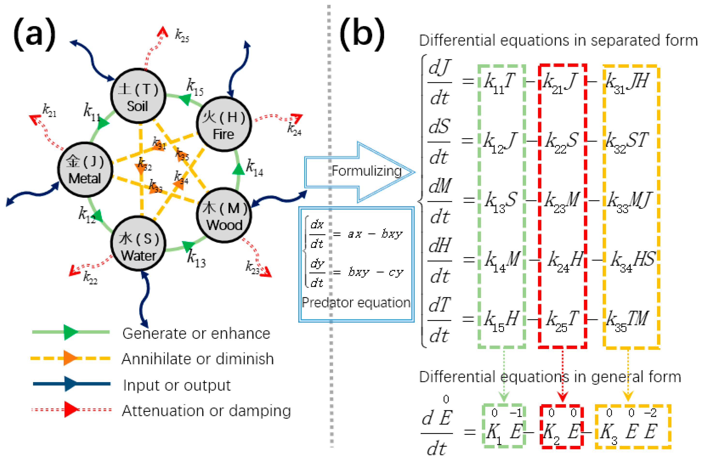
Motivated by this challenge, we propose a novel class of symmetric differential equations grounded in symmetry principles. Figure 2 illustrates the conceptual development of our symmetric differential equation system.
As shown in Figure 2a, we begin with the traditional Wuxing (Five Elements) framework from Chinese philosophy, which encodes a closed and symmetric logic of generation and inhibition among five elemental components: Metal (J), Water (S), Wood (M), Fire (H), and Soil (T). In this cyclical structure, each element either promotes (generates) or suppresses another, forming a self-contained symmetric system.
To translate this logic into a dynamic model, we reformulate the framework by incorporating self-decay and input-output nodes, while also drawing inspiration from predator equation (Equation (7)). The resulting system is a distributed set of differential equations, as depicted in Figure 2b and formalized in Equation (8). For instance, in the Wuxing logic, Soil gives rise to Metal (e.g., ore is extracted from soil), whereas Fire can melt and thereby subdue Metal. This interaction leads to the first equation in (8): d J / d t = k 11 T k 21 J k 31 J H . Here, the second term represents a self-decay component, introduced to stabilize the system in analogy with the damping mechanisms in ecological equations.
d x d t = a x b x y d y d t = b x y c y
d J d t = k 11 T k 21 J k 31 J H d S d t = k 12 J k 22 S k 32 S T d M d t = k 13 S k 23 M k 33 M J d H d t = k 14 M k 24 H k 34 H S d T d t = k 15 H k 25 T k 35 T M
Let E = {J, S, M, H, T} denote the set of elemental states, and define three parameter sets: K 1 = { k 11 , k 12 , k 13 , k 14 , k 15 } , K 2 = { k 21 , k 22 , k 23 , k 24 , k 25 } , K 3 = { k 31 , k 32 , k 33 , k 34 , k 35 } , Then, the system in Equation (8) can be rewritten in a compact form as Equation (9).
d E d t = K 1 E K 2 E K 3 E E
It is important to note that the ordering of elements within the vector E differs depending on the context and position in the equation, and thus cannot be trivially unified. However, if we consider a cyclic permutation of these elements across different positions, Equation (9) can be generalized into a rotationally symmetric form, denoted as Equation (10) (see Figure 2b).
d E 0 d t = K 1 0 E 1 K 2 0 E 0 K 3 0 E 0 E 2
This general formulation permits arbitrary extension in the number of elements and customization of their interaction rules, provided that the cyclic structure is preserved. Consequently, the generalized form (Equation (10)) possesses broader applicability. Due to the structural similarities among such symmetric differential systems, analytical results obtained from Equation (8) can naturally be extended to the broader family defined by Equation (10).
This framework offers several distinct advantages. First, it possesses perfect symmetry, enabling bidirectional signal propagation, which eliminates the need for gradient-based calculations. Second, the structural design is based on differential equations, thereby ensuring a high degree of biological plausibility. According to our design, network training no longer depends on global gradient computation but instead relies solely on local signal comparisons. Third, the topological structure of the system can maintain complete symmetry, allowing for a signal propagation mechanism analogous to the chain rule and enabling pointwise parameter adjustment with high precision. Fourth, the symmetric differential equations themselves inherently possess nonlinear characteristics, eliminating the need to introduce additional nonlinear activation functions such as ReLU or Sigmoid.
Table 1 illustrates the differences and connections between the traditional multilayer perceptrons and symmetric differential equation neural networks.
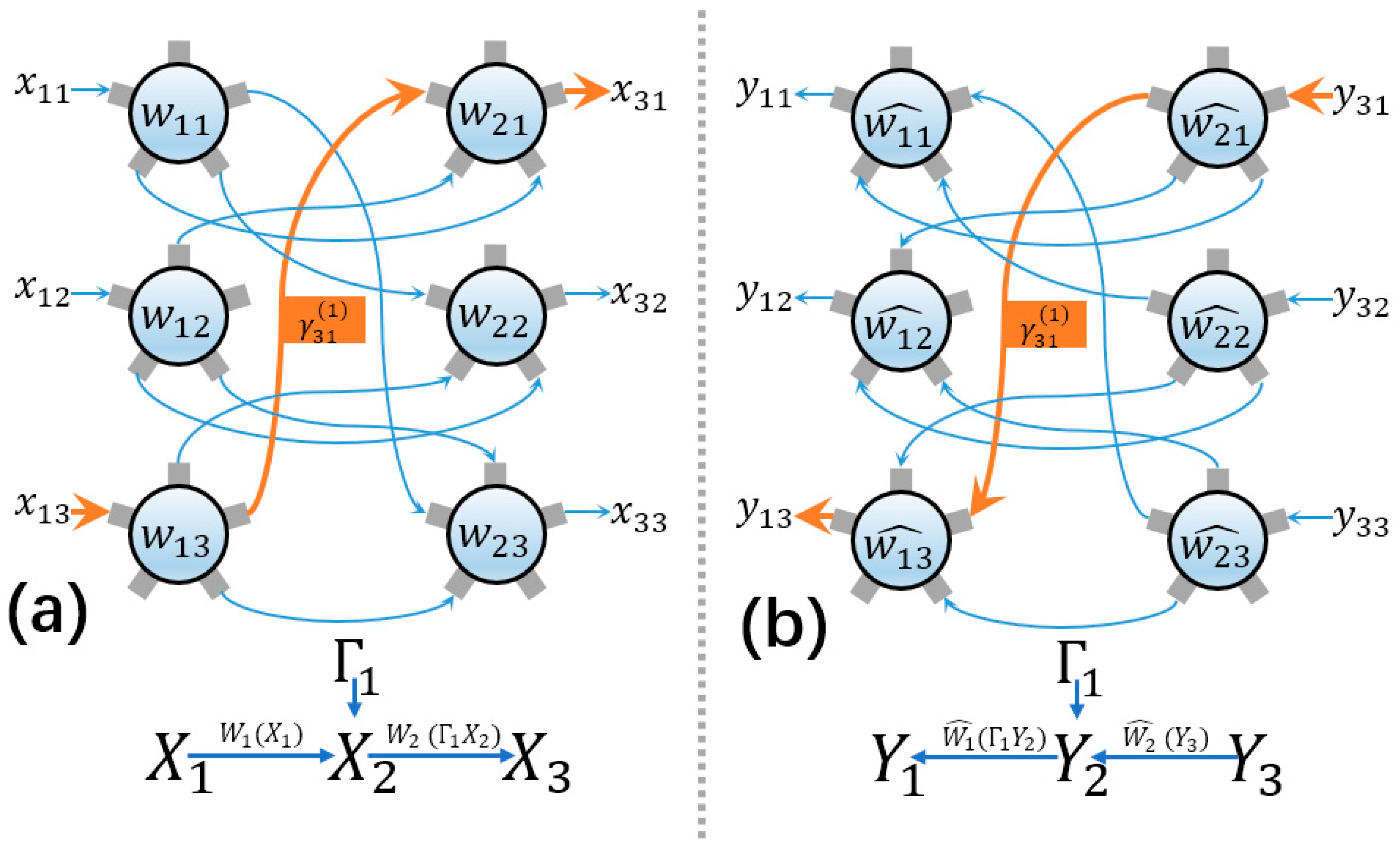
Figure 3 illustrates a neural network architecture based on symmetric differential equations. This structure aligns with the multilayer perceptron (MLP) shown in Figure 1, as both comprise three input nodes, three output nodes, and two layers of nonlinear transformations. A comparison between Figure 1 and Figure 3 reveals that we have replaced the original simple neurons with symmetric differential equations.
In Figure 3a, w 11 , w 12 , w 13 , w 21 , w 22 , w 23 represents the symmetric differential equations introduced in Figure 2, it functionally corresponds to the nonlinear function f 1 and f 2 in Figure 1c. These systems are inherently nonlinear, eliminating the need for additional nonlinear activation functions. A forward signal propagation path and a backward propagation path are explicitly indicated in Figure 3, which follows the same logic as in Figure 1. In Figure 3b, w 11 ^ , w 12 ^ , w 13 ^ , w 21 ^ , w 22 ^ , w 23 ^ denotes the inverse symmetric differential equation, it functionally corresponds to the nonlinear function f 1 ~ and f 2 ~ in Figure 1d. It is mathematically identical to the forward equation, with the only difference being that the signal propagates in the opposite direction to that of the forward system. Additionally, connection coefficients Γ 1 are incorporated between the neurons in Figure 3, serving the same function as the corresponding coefficients in a traditional MLP. Thus, we have structurally constructed a neural network based on symmetric differential equations that resembles an MLP.

3.2. Causal Distance

As previously discussed, the inherent symmetry of the system allows for straightforward reversibility. This naturally raises the question: What are the invariants in this reversal process? This is a crucial and underexplored issue. Building on our analysis of the network’s topology, we introduce the concept of causal distance, proposing it as the system’s key invariant. We argue that causal distance plays a decisive role in constructing reversible systems and serves as a guiding principle in maintaining system-level symmetry.
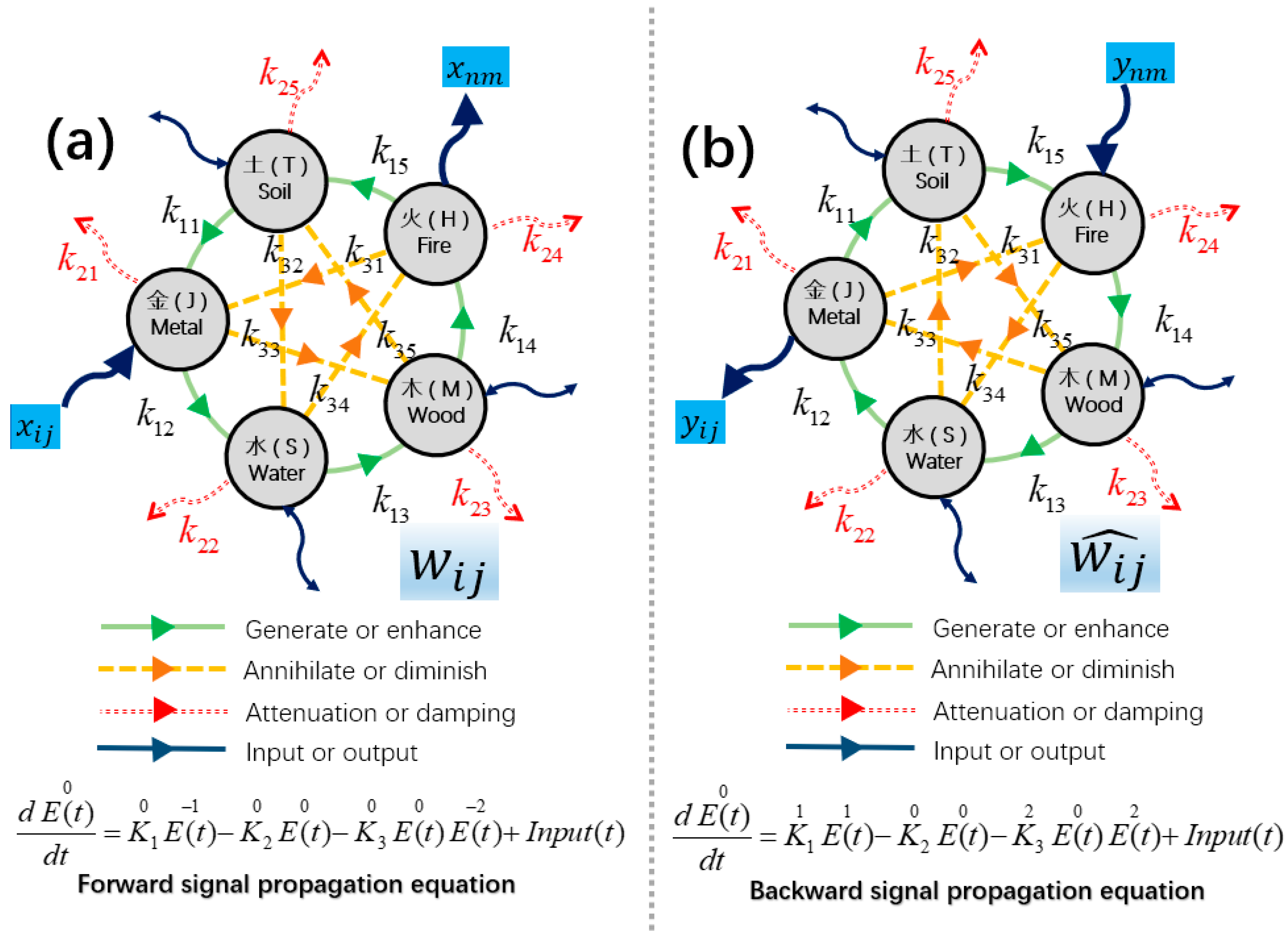
Figure 4 presents the structure of symmetric differential equations for both forward and backward propagation. In Figure 4a, x i j and x n m denote the input and output signals in the forward propagation process, respectively. In Figure 4b, y n m and y i j denote the input and output signals in the backward (error) propagation process.
According to the structure of the system, we can establish the forward signal input equation of the system:
d E ( t ) 0 d t = K 1 0 E ( t ) 1 K 2 0 E ( t ) 0 K 3 0 E ( t ) 0 E ( t ) 2 + I n p u t ( t )
In Figure 2a, we show the logical relationship of the five elements. For example, water can generate wood because plants can grow with water, and metal can restrain wood because an ax made of metal can cut down trees. Based on this logical relationship, we obtain the third equation d M / d t = k 13 S k 23 M k 33 M J in Figure 2b. If we reverse this causal relationship, it becomes that wood can generate water and wood can restrain metal; similarly, fire can generate wood, and soil restrains wood. When all causal relationships are totally reversed, we can obtain the logical structure of Figure 4b and Equation (12):
d J d t = k 12 S k 21 J k 33 J M d S d t = k 13 M k 22 S k 34 S H d M d t = k 14 H k 23 M k 35 M T d H d t = k 15 T k 24 H k 31 H J d T d t = k 11 J k 25 T k 32 T S
According to our definition, the system’s signals can propagate in both directions. Based on the system’s topological structure, we define the backward equation containing signal propagation term:
d E ( t ) 0 d t = K 1 1 E ( t ) 1 K 2 0 E ( t ) 0 K 3 2 E ( t ) 0 E ( t ) 2 + I n p u t ( t )
Although this structure is the result of reversing Figure 1a, their topological link relationship has not changed. The equations obtained in Figure 4b are consistent with the equations in Figure 4a in mathematical structure, and only the order of elements has changed.
When a signal is input into Equation (10) (Figure 4a), an output signal is obtained. This input-output relationship is a nonlinear function, corresponding to the f n function in Figure 1c. Similarly, Equation (12) (Figure 4b) is also equivalent to a nonlinear function for the input signal, corresponding to the f n ~ function in Figure 1d.
This mirrored topological structure ensures that Figure 2a and Figure 2b align with the forward and backward propagation diagrams shown in Figure 1c and Figure 1d, respectively.
In the symmetric differential equation system we constructed, a set of multivariate coupled ordinary differential equations (ODEs) is involved, within which the variables exhibit intricate interdependencies. These dependencies are not only directional but also hierarchical in nature, manifesting a chain-like propagation pattern. In such systems, changes in a particular variable do not instantaneously influence all others; rather, the effects are transmitted progressively along directed paths, undergoing accumulation, attenuation, or feedback modulation during the propagation. To characterize this feature, we introduce the concept of a causal interaction chain and further define a novel structural metric termed causal distance.
Causal distance refers to the minimum number of intermediate variables required for one variable to influence another within a predefined causal propagation graph. For example, if the derivative of variable J directly depends on variable T, the causal distance between them is defined as 1. Conversely, if variable H affects J only indirectly through T, then the causal distance from H to J is 2. This unified perspective not only enhances our understanding of the intrinsic structural dynamics of ODE systems but also provides a rich toolkit for modeling complex networked systems. Specifically, two key insights emerge: (1) variables with shorter causal distances exhibit more direct influence and elicit faster system responses; (2) variables connected through longer causal chains tend to produce delayed responses, making them more susceptible to accumulation effects.
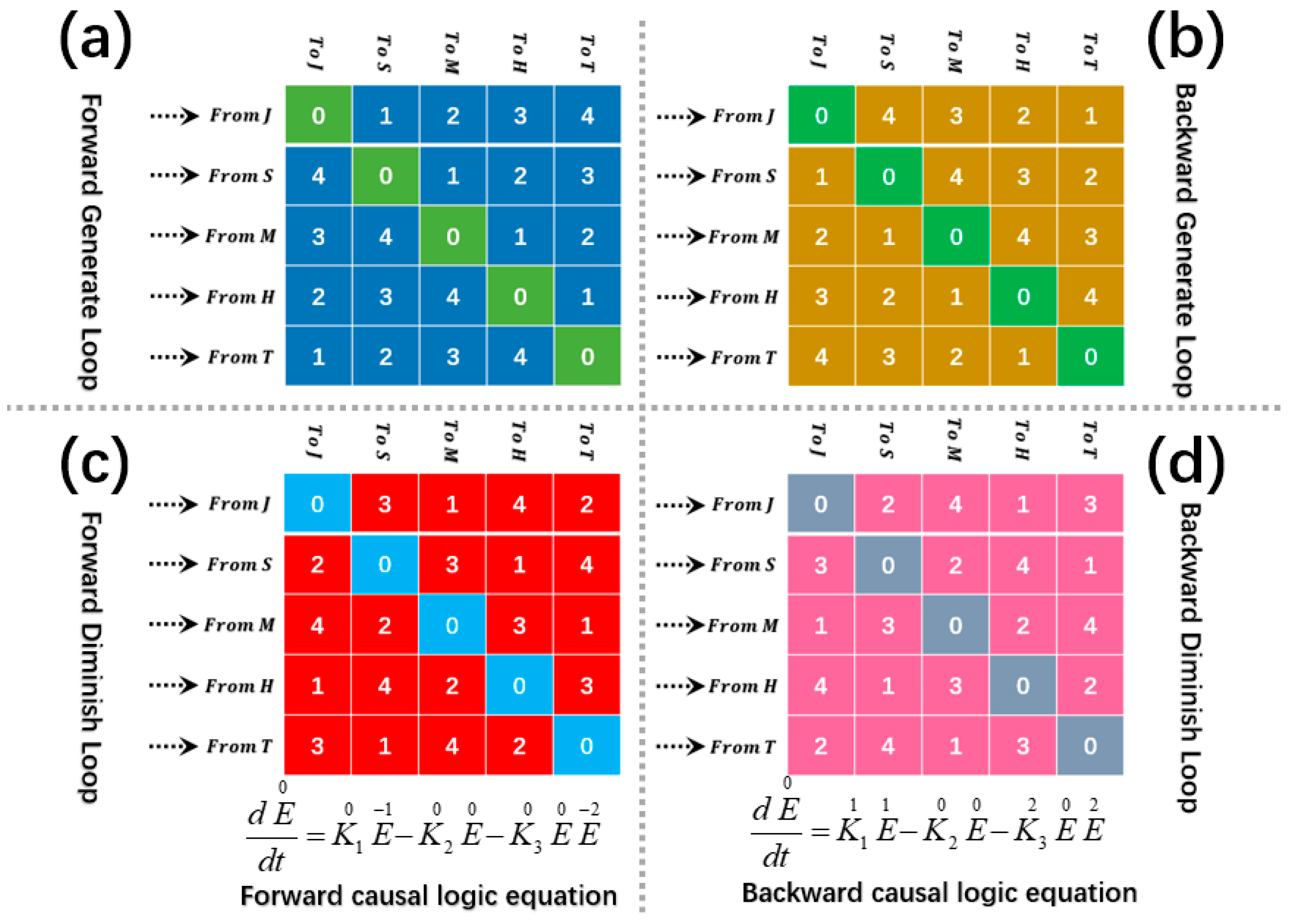
In Equation (7), two loops are present. The first loop represents a generative loop among elements ( J S M H T J ), while the third term embodies an inhibitory loop ( J M T S H J ).
Figure 5 illustrates the causal distances within these two loops, derived from both the forward and reverse formulations of the causal equations. Specifically, Figure 5a presents the causal distance matrix for the generative loop in the forward causal equation; Figure 5b corresponds to the same loop in the reverse causal equation; Figure 5c displays the causal distances for the inhibitory loop in the forward equation; and Figure 5d shows the inhibitory loop in the reverse formulation. As observed, the causal distances between corresponding elements are perfectly symmetric in both formulations, reflecting the inherent structural symmetry of the differential equation system we designed.
Building upon this theoretical framework, we extend the concept of causal distance to describe the interactions between system parameters and state variables. For instance, in Figure 4a, variable J directly depends on variable T, with a coupling coefficient k 11 ; meanwhile, T is regulated by another parameter k 15 through its effect on variable H. Under this configuration, a causal distance can be defined between system parameters and state variables. Specifically, the causal distance between k 11 and J is considered to be 1, indicating a rapid and direct response of J to perturbations in k 11 . In contrast, since the effect of k 15 on J is mediated by T, it entails a longer causal path and hence a lower sensitivity of J to changes in k 15 .
This leads to an intuitive conclusion: the influence of directly coupled parameters (e.g., k 11 ) on system variables (e.g., J) is more immediate and pronounced, while parameters involved in multi-stage indirect dependencies (e.g., k 15 ) exhibit weaker impacts due to transmission attenuation. This observation lays the groundwork for a causal-distance-based theory, where both inter-variable dependencies and parameter-variable couplings can be evaluated in terms of their causal distances. In general, shorter causal distances imply more direct and stronger regulatory effects, whereas longer distances tend to yield diminished sensitivities due to intermediate information loss.
This theoretical framework offers several key advantages:
  • Reduction in analytical complexity: By assigning causal distances to each dependency relationship, the system’s analysis can adopt a strategy analogous to Principal Component Analysis (PCA) [18], ranking and filtering the contributing factors. Variables or parameters with short causal distances often constitute the core drivers of the system, while those with long distances and marginal influence can be safely ignored during preliminary modeling, thereby simplifying system analysis significantly.
  • Quantification of influence strength: Causal distance provides not only a qualitative description of transmission paths but also a means for quantitative assessment when combined with coupling coefficients. In the aforementioned example, the direct dependency of J on k11 results in a strong and rapid effect, while the impact of k15 is attenuated due to intermediate transmission. This approach introduces a quantitative scale for dynamical systems, facilitating accurate identification of key control parameters in sensitivity analysis or parameter tuning tasks.
  • Unified structural representation: Extending causal distance to cover parameter-variable dependencies enables a unified analytical tool that can describe both the internal causal feedback chains among variables and the regulatory effects of system parameters. This unification deepens our understanding of the “structural lag” phenomenon in complex systems and provides a theoretical foundation for the design of control strategies.
In summary, the development of the causal distance framework elucidates the mechanisms of direct and indirect interactions among variables and provides an intuitive and effective metric for assessing sensitivity and influence strength. By focusing on dominant causal chains and excluding negligible effects, the model’s analytical clarity and explanatory power are greatly enhanced. This methodology shares conceptual similarities with PCA, emphasizing the ranking and selection of impactful factors to reduce system dimensionality and extract principal driving patterns, thereby improving the tractability and efficiency of complex system research.

4. Experiment

4.1. Forward and Backward Signal Design

In the framework of symmetric differential equations, we define the system’s zero state as the state in which it resides at its fixed point. When an external signal is injected, the system deviates from this fixed point, and the resulting deviation is regarded as the corresponding output signal. This can be formally defined as follows:
D ( t ) = E ( t ) B 0
where D(t) denotes the deviation from the fixed point, E(t) represents the real-time signal of the system element, and B 0 is the fixed point of the system. The fixed point B 0 can be determined by solving the following equation:
B 0 K 1 ¯ K 2 ¯ K 3 ¯
In Equation (15), K 1 ¯   K 2 ¯   K 3 ¯ , denote the average values of the three groups of parameters described earlier. When the parameters within each group are identical, Equation (15) provides an exact solution. Although Equation (15) only gives an approximate fixed point of Equation (9), it reveals the qualitative relationship between the fixed point B and the parameters K 1 , K 2 and K 3 . Specifically, B 0 is positively correlated with K 1 ; as K 1 increases monotonically. Conversely, B 0 is negatively correlated with K 2 and K 3 ; an increase in either K 2 or K 3 results in a monotonic decrease in B 0 .
Similarly, D ^ ( t ) is determined by the back-propagated element value E ^ ( t ) and the back-propagated fixed point B ^ 0 .
D ^ ( t ) = E ^ ( t ) B ^ 0
According to our design, the signal propagating through the forward network is D(t), and the signal propagating through the backward network is D ^ ( t ) By comparing the differences between these two signals, we can effectively train the neural network.

4.2. Two Different Learning Methods

In our previous work, we proposed two distinct approaches for training neural networks. The first method involves modifying the system’s fixed points [19], while the second adjusts the connection weights between neurons [20]. Both methods rely on error signals propagating backward through the network, a mechanism we refer to as Backward Signal Propagation (BSP). Through BSP, system parameters can be precisely adjusted based on the signals propagated within the network. Below, we briefly introduce how the two types of signals in the system can be utilized to tune parameters.

4.2.1. First Learning Method: Adjusting the System’s Fixed Points

The first training approach modifies the fixed points of the system. As discussed earlier, the fixed points of the system are tightly coupled to three groups of parameters defined in Equation (9). Therefore, we proposed a method based on distributed PID control to independently regulate each group of parameters, and experimental results validated the success of this approach.
Based on the forward and reverse signals propagated within time T , we can define a correlation variable G 1 .
G 1 = 0 T D ( t ) d t 0 T D ^ ( t ) d t
In Equation (17), G 1 is the product of the forward signal integral and the backward signal integral, which reflects the difference between the forward and backward signals. If the two signals have opposite signs, it means that the parameters at the corresponding position should be adjusted to reduce the output; if the signs are the same, it means that the parameters at the corresponding position should be adjusted to increase the output.
Since G 1 may exceed a certain limit, we use the inverse tangent function (other similar functions are also possible) to limit it and obtain G 2
G 2 = a t a n ( G 1 k t ) / k t
k t is the adjustment parameter, and G 2 is the adjusted correlation value. The parameter can be adjusted based on G 2 .
K 3 _ n e w = K 3 _ o l d e x p ( G 2 )
In Equation (19), we used the parameter K 3 as an example to illustrate the tuning process. The correspondence between the adjustment components and the system parameters was determined according to the causal distance between them. Initial results confirmed the effectiveness of the approach. Extending this method to multiple parameter groups requires the implementation of distributed PID control strategies.
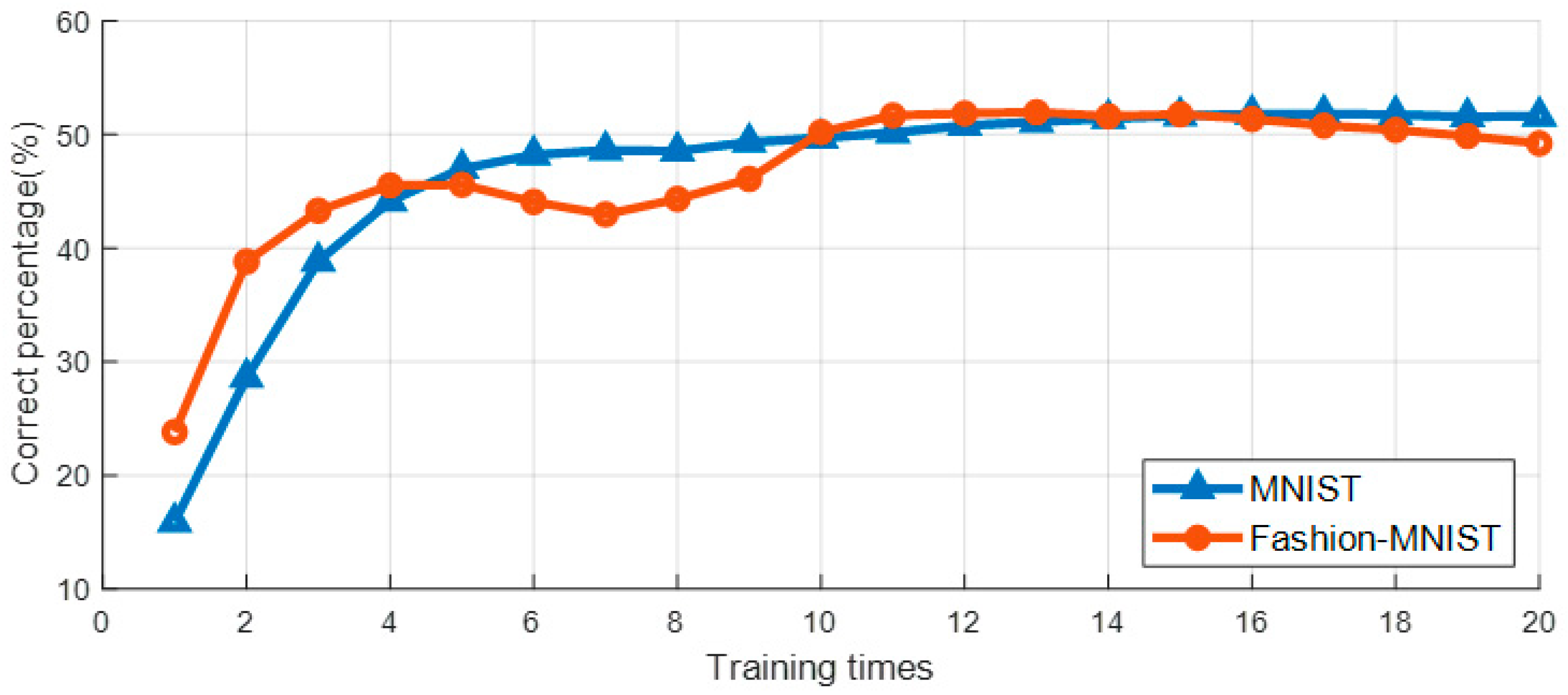
Figure 6 presents the training results on the MNIST and Fashion-MNIST datasets, with the number of neurons in each layer set to {784,839,283,96,32,10}. The accuracy on both datasets reaches approximately 50%. A notable difference, however, is that training on MNIST exhibits greater stability, which can be attributed to the intrinsic characteristics of the dataset. By contrast, Fashion-MNIST was deliberately designed to introduce higher training complexity, resulting in larger fluctuations in the accuracy curve. Importantly, the relatively low accuracy observed here does not stem from limitations of the training method itself, but rather from structural deficiencies in the system’s topology. To address this, we further introduced a second training method, which simultaneously improves both the training process and the system architecture.

4.2.2. Second Learning Method: Adjusting Neuronal Connections

The second approach focuses on tuning the connection parameters between neurons, akin to the training process of traditional multilayer perceptrons (MLPs). In particular, our analysis of Figure 2b led to a simple and efficient parameter update rule (Equation (2)). A key limitation of this rule in conventional architectures is the inability to propagate error signals globally. However, within the BSP framework, the signal D ^ t naturally serves as a globally propagated error signal. This enables each neuron to apply the learning rule from Equation (2) effectively. Assuming that the inter-neuronal connection weights are denoted by C, the forward propagation equation of the system can be written as Equation (20).
d E ( t ) 0 d t = K 1 0 E ( t ) 1 K 2 0 E ( t ) 0 K 3 0 E ( t ) 0 E ( t ) 2 + C I n p u t ( t )
The backward propagation equation is modified as follows:
d E ( t ) 0 d t = K 1 1 E ( t ) 1 K 2 0 E ( t ) 0 K 3 2 E ( t ) 0 E ( t ) 2 + C I n p u t ( t )
In Equations (20) and (21), the coefficients C remains consistent across corresponding positions, ensuring causal consistency before and after connections. To maintain a one-to-one correspondence between cause and effect, each neuron’s synaptic connections are strictly one-to-one. Compared with the fully connected structure of traditional MLPs, the connections in the Wuxing neural network are significantly sparser.
According to Equation (2), we can also give a similar training method. Assume that the system has n layers, where the forward output signal of the i t h layer neuron is D i ( t ) , and similarly, the backward output signal of the i t h layer neuron is D ^ i ( t ) . If the calculation time is T , we can define a variable G 1 :
G 1 = 0 T D i ( t ) d t 0 T D ^ i + 1 ( t ) d t
In Equation (22), G 1 represents the causal quantity of the connection parameters between the neurons in the i t h layer and the neurons in the i + 1 t h layer.
Since G 1 may exceed a certain limit, we use the inverse tangent function (other similar functions are also possible) to limit it and obtain G 2 , as shown in Eqation (18).
k t is the adjustment parameter, G 2 is the adjusted correlation value. The parameter can be adjusted based on G 2 .
C n e w = C o l d + G 2
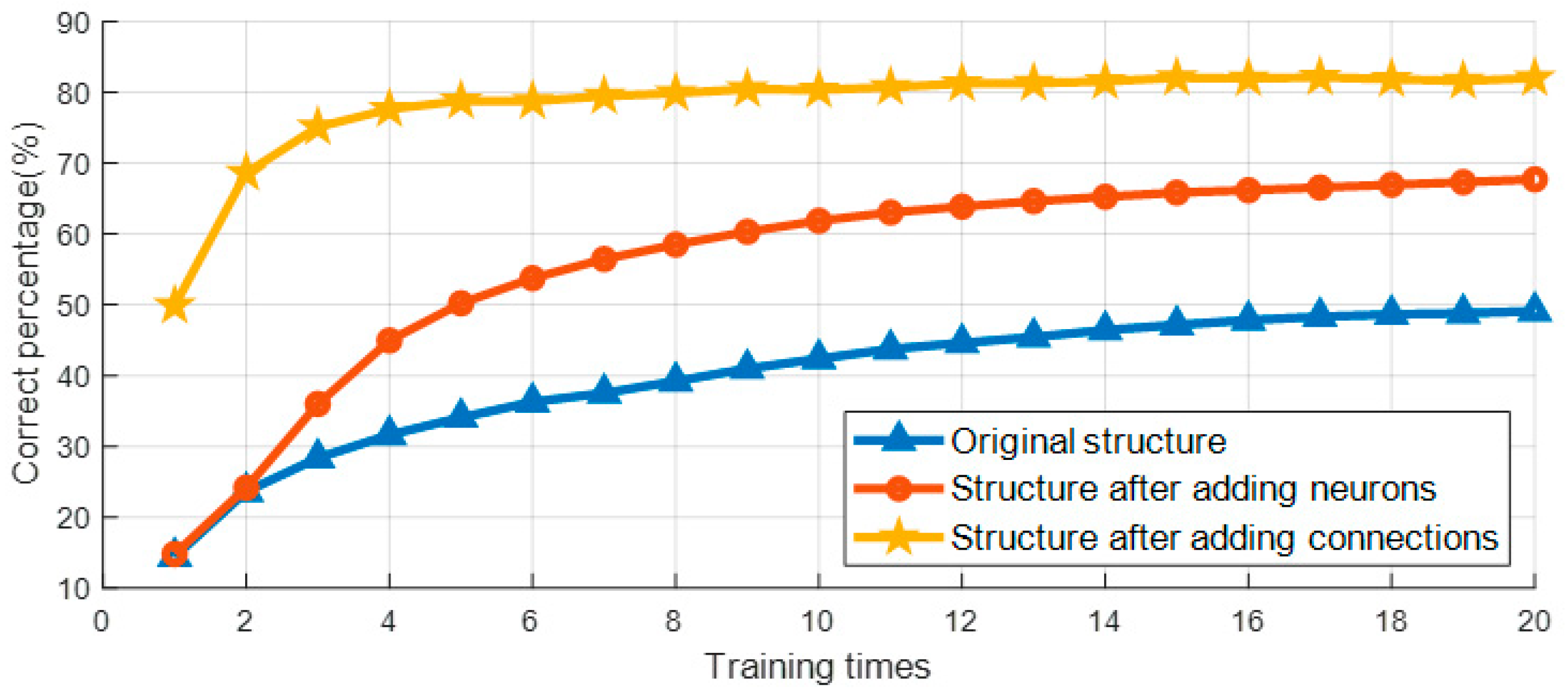
Based on Equation (23). and using the same network structure as in Method 1, we trained the MNIST dataset and achieved an accuracy of approximately 50% (corresponding to the blue curve in Figure 7). If the number of neurons is increased to {784,1048,353,119,40,10}, the accuracy can be further improved to approximately 70% (corresponding to the red curve in Figure 7). However, in this configuration, each neural node is connected to only one node in the subsequent layer. If instead each node is allowed to connect with multiple nodes in the next layer, the network with {784,300,300,10} neurons can achieve an accuracy of 82% (corresponding to the yellow curve in Figure 7). This result demonstrates that under multi-connection settings, we are able to employ fewer neurons, thereby effectively reducing computational complexity while also achieving faster training speed.
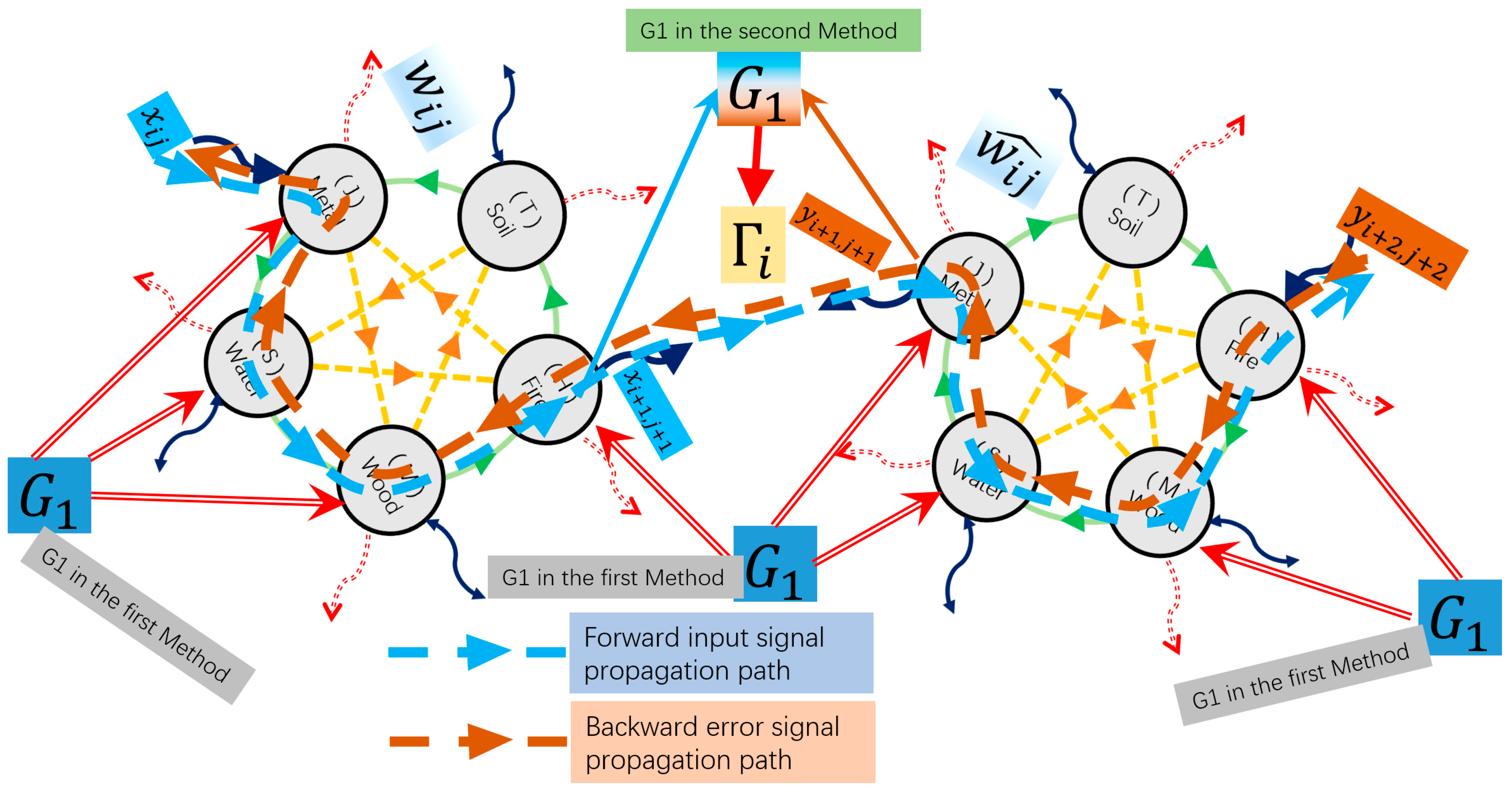
Figure 8 illustrates the forward signal propagation path and the backward error signal propagation path. In the two training methods we designed, a new variable G 1 is constructed through the cooperative interaction between the forward-propagating signal D ( t ) and the backward-propagating error signal D ^ ( t ) This variable is defined as the error modulation signal. Due to the symmetry of the network structure, G 1 can naturally propagate throughout the network topology, thereby enabling effective adjustment of parameters at different locations. Because the construction of G 1 is directly based on the topological relationships among local signals, it accurately reflects the true impact of each parameter on the global error. Consequently, the adjustment method based on G 1 offers both strong locality and significant advantages in efficiency and accuracy.
It should be emphasized that in the generative loop, which serves as the dominant loop of the system, each element in the causal chain simultaneously experiences both the forward and backward signals. The specific definition of G 1 differs between the two training methods: in method 2, for example, the parameters Γ i to be adjusted are located between two neurons, so G 1 must be defined using the signals from both neurons ( x i + 1 , j + 1   a n d   y i + 1 , j + 1 ). These two training methods are not the end point; rather, they demonstrate that, based on the BSP framework, a wider variety of learning mechanisms can be designed to further enhance training performance.
In summary, according to the signal propagation process, we can give the following training steps:
  • Feed the input signal into the network. Compute the forward propagation of the signal through all layers.
  • Compute the error signal based on the difference between the output and the target at the output layer.
  • Propagate the error signal backward through the network.
  • At each node, combine the forward signal and the backward error signal to construct the modulation variable G1.
  • Update the system parameters according to the computed modulation variable G1.
  • Repeat steps 1–5 until convergence criteria are satisfied (e.g., error or maximum epochs).

5. Summary

In this work, we conducted an in-depth analysis of the two core mechanisms underpinning the effectiveness of the backpropagation algorithm: differentiation and the chain rule. The former enables a mathematical characterization of causal influence among variables in any differentiable function, while the latter allows this causal pathway to be propagated layer by layer in complex network architectures, thus enabling system-level error feedback. This combination of formal rigor and structural adaptability is what establishes BP as a dominant training strategy in deep learning.
To propose an alternative approach that combines training efficiency with biological plausibility, we introduced a novel learning framework based on symmetric differential equations, termed Backward Signal Propagation (BSP). Our contributions can be summarized in two main innovations:
First, by leveraging the local differentiability of differential equations, we express causal effects without requiring explicit gradient computation. This allows the training process to be naturally embedded within the dynamical evolution of signal propagation.
Second, we introduced the concept of causal distance and demonstrated its consistency between the forward and backward subsystems (i.e., causal distance invariance) in symmetric network structures. This provides theoretical support for the global propagation of error signals.
Within this network architecture, the system operates based on two types of signals only: the forward-propagating input signal and the backward-propagating error signal. From these, we generate the error modulation signal G 1 , which is used to locally and precisely adjust all system parameters. Causal distance not only provides the geometric foundation for error signal propagation but also indicates the preferential directions for parameter updates. Experimental results confirm that adjusting parameters closer (in causal distance) to G 1 leads to more pronounced training responses, validating the local efficiency of the BSP method.
Overall, the BSP framework plays a foundational role for symmetric differential networks, akin to the role of BP in traditional multilayer perceptrons. Its introduction not only offers a biologically feasible training mechanism but also opens a new pathway toward constructing neural systems that are highly reversible, structurally symmetric, and signal-driven. Future research will focus on further optimizing the engineering realization of BSP, including improving training efficiency, enhancing generalization capabilities, and extending its application to more complex network architectures and task scenarios—ultimately paving the way for its deployment in a broad range of intelligent systems.

Author Contributions

Conceptualization, K.J.; Methodology, K.J.; Validation, K.J.; Formal analysis, K.J.; Investigation, K.J.; Writing—original draft, K.J.; Writing—review & editing, K.J.; Supervision, Z.F.; Project administration, K.J. All authors have read and agreed to the published version of the manuscript.

Funding

This research received no external funding.

Data Availability Statement

Data is available in a publicly accessible repository. It can be downloaded from: https://yann.lecun.org/exdb/mnist/index.html (accessed on 4 August 2025).

Acknowledgments

Thanks to China Scholarship Council (CSC) for their support during the pandemic, which allowed me to get through those difficult days and give me the opportunity to put my past ideas into practice, ultimately resulting in the article I am sharing with you today.

Conflicts of Interest

The authors declare no conflicts of interest.

Abbreviations

The following abbreviations are used in this manuscript:
BSPBackward signal propagation
BPBackpropagation
MLPMultilayer perceptrons
MNISTModified National Institute of Standards and Technology database

References

  1. Rosenblatt, F. The perceptron: A probabilistic model for information storage and organization in the brain. Psychol. Rev. 1958, 65, 386. [Google Scholar] [CrossRef]
  2. Marvin, M.; Seymour, A.P. Perceptrons; MIT Press: Cambridge, MA, USA, 1969; Volume 6, p. 7. [Google Scholar]
  3. Rumelhart, D.E.; Hinton, G.E.; Williams, R.J. Learning representations by back-propagating errors. Nature 1986, 323, 533–536. [Google Scholar] [CrossRef]
  4. Hochreiter, S. The vanishing gradient problem during learning recurrent neural nets and problem solutions. Int. J. Uncertain. Fuzziness Knowl.-Based Syst. 1998, 6, 107–116. [Google Scholar] [CrossRef]
  5. Deng, J.; Dong, W.; Socher, R.; Li, L.J.; Li, K.; Li, F.-F. Imagenet: A large-scale hierarchical image database. In Proceedings of the 2009 IEEE Conference on Computer Vision and Pattern Recognition, Miami, FL, USA, 20–25 June 2009; IEEE: Piscataway, NJ, USA, 2009. [Google Scholar]
  6. Raina, R.; Madhavan, A.; Ng, A.Y. Large-scale deep unsupervised learning using graphics processors. In Proceedings of the ICML ‘09: Proceedings of the 26th Annual International Conference on Machine Learning, Montreal, QC, Canada, 14–18 June 2009. [Google Scholar]
  7. LeCun, Y.; Bengio, Y.; Hinton, G. Deep learning. Nature 2015, 521, 436–444. [Google Scholar] [CrossRef] [PubMed]
  8. Bottou, L. Large-scale machine learning with stochastic gradient descent. In Proceedings of the COMPSTAT’2010: 19th International Conference on Computational Statistics, Paris, France, 22–27 August 2010; Keynote, Invited and Contributed Papers. Springer: Berlin/Heidelberg, Germany, 2010. [Google Scholar]
  9. Kingma, D.P.; Ba, J. Adam: A method for stochastic optimization. arXiv 2014, arXiv:1412.6980. [Google Scholar]
  10. Hinton, G. The forward-forward algorithm: Some preliminary investigations. arXiv 2022, arXiv:2212.13345. [Google Scholar] [CrossRef]
  11. Lillicrap, T.P.; Santoro, A.; Marris, L.; Akerman, C.J.; Hinton, G. Backpropagation and the brain. Nat. Rev. Neurosci. 2020, 21, 335–346. [Google Scholar] [CrossRef] [PubMed]
  12. Crick, F. The recent excitement about neural networks. Nature 1989, 337, 129–132. [Google Scholar] [CrossRef] [PubMed]
  13. Stork. Is backpropagation biologically plausible? In Proceedings of the International 1989 Joint Conference on Neural Networks, Washington, DC, USA, 18–22 June 1989; IEEE: Piscataway, NJ, USA, 1989. [Google Scholar]
  14. Kun, J. A Neural Network Framework Based on Symmetric Differential Equations. ChinaXiv 2024. ChinaXiv:202410.00055. [Google Scholar]
  15. Jiang, K. From Propagator to Oscillator: The Dual Role of Symmetric Differential Equations in Neural Systems. arXiv 2025, arXiv:2507.22916. [Google Scholar]
  16. Izhikevich, E.M. Dynamical Systems in Neuroscience; MIT Press: Cambridge, MA, USA, 2007. [Google Scholar]
  17. Olver, P.J. Equivalence, Invariants and Symmetry; Cambridge University Press: Cambridge, UK, 1995. [Google Scholar]
  18. Abdi, H.; Williams, L.J. Principal Component Analysis. Wiley Interdiscip. Rev. Comput. Stat. 2010, 2, 433–459. [Google Scholar] [CrossRef]
  19. Jiang, K. A Neural Network Training Method Based on Distributed PID Control. Symmetry 2025, 17, 1129. [Google Scholar] [CrossRef]
  20. Jiang, K. A Neural Network Training Method Based on Neuron Connection Coefficient Adjustments. arXiv 2025, arXiv:2502.10414. [Google Scholar]
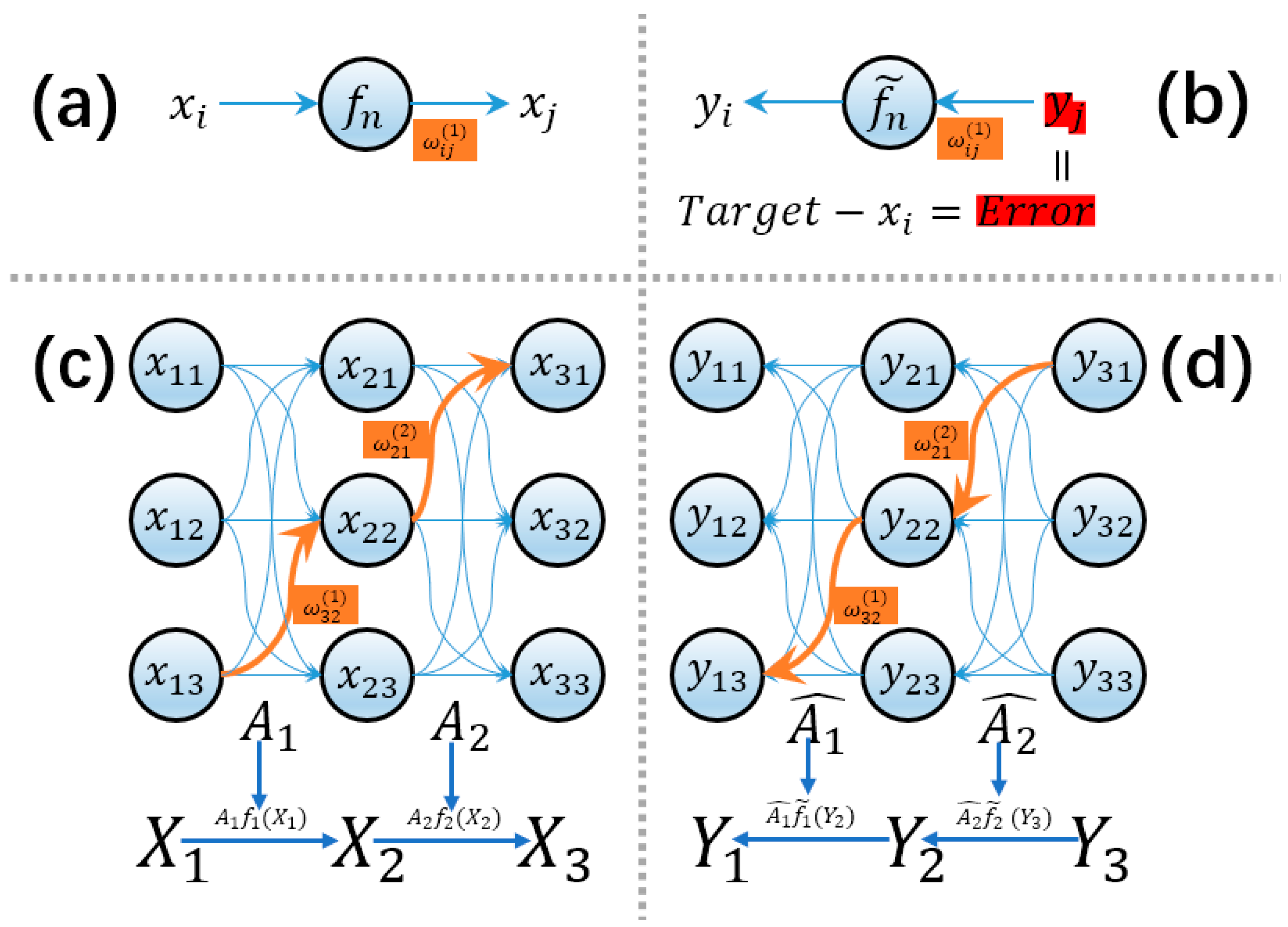
Figure 1. Signal propagation process in traditional neural networks. (a) The signal propagation process in a single neuron. (b) The backward propagation of the error signal in a single neuron. (c) The signal propagation process in multilayer perceptron. (d) The backward propagation of the error signal in multilayer perceptron.
Algorithms 18 00594 g001
Figure 2. From Wuxing logic to symmetric differential equations. (a) Traditional Wuxing logic posits that the world is composed of five distinct elements that interact through generative and inhibitory relationships, forming the logical framework of the universe. The logical structure depicted in the figure deviates from the traditional model by incorporating self-attenuation terms and creating interfaces for external input and output signals. In this system, there are five nodes, each capable of serving as an input or output. However, to prevent signal interference, a node can either receive input or generate output at any given time, but not both simultaneously. (b) By combining the Wuxing logic with the predator-prey equation, we can derive a set of differential equations. The symmetry of the system is carefully preserved throughout this transformation process. As a result, both the traditional Five Elements logic and the predator-prey equation are modified, ultimately leading to a set of fully symmetrical equations. For clarity, these equations are presented in a generalized format, with the numbers above the elements and parameters indicating the offset of each loop.
Algorithms 18 00594 g002
Figure 3. Signal propagation in neural networks based on symmetric differential equations. (a) Signal propagation in symmetric differential equation neural networks. Since differential equations have natural nonlinear characteristics, we do not need to introduce additional functions, thus building a more biologically plausible neural network structure. (b) Backward error signal propagation in symmetric differential equation neural networks. It can be seen that in the external connections of neurons, we have adopted a method that is completely symmetrical with for-ward propagation, but how to reverse the internal relationship of neurons so that the system can achieve reverse causality will be the issue next.
Algorithms 18 00594 g003
Figure 4. Forward and backward signal propagation in symmetric differential equations. (a) Forward signal propagation in symmetric differential equations. (b) Backward signal propagation in symmetric differential equations.
Algorithms 18 00594 g004
Figure 5. Causal distance between elements in the forward and reverse systems. (a) Causal distance table in the generative loop in the forward propagation equation. (b) Causal distance table in the generative loop in the backward propagation equation. (c) Causal distance table in the diminish loop in the forward propagation equation. (d) Causal distance table in the diminish loop in the backward propagation equation.
Algorithms 18 00594 g005
Figure 6. Accuracy curves trained on MNIST and Fashion MNIST.
Algorithms 18 00594 g006
Figure 7. Accuracy curves trained on different structures.
Algorithms 18 00594 g007
Figure 8. Forward and backward signal propagation paths. The red dashed line represents the forward input signal propagation path, while the blue dashed line represents the backward error propagation path. Due to the reversibility of the system, these two paths are completely symmetrical.
Algorithms 18 00594 g008
Table 1. Comparison between multilayer perceptron and symmetric differential equation neural networks.
Multilayer PerceptronSymmetric Differential Equation Neural Networks
Signal sourceDefined by input signal and nonlinear functionGenerate perturbation signal from input signal
Nonlinear propertyActivation functionNatural property of the system
Causal tracing methodsDerivative operationDifferentiability of equations
Traversing the topologyChain propagation lawCausal distance invariance
Disclaimer/Publisher’s Note: The statements, opinions and data contained in all publications are solely those of the individual author(s) and contributor(s) and not of MDPI and/or the editor(s). MDPI and/or the editor(s) disclaim responsibility for any injury to people or property resulting from any ideas, methods, instructions or products referred to in the content.