Parallelizing the Computation of Grid Resistance to Measure the Strength of Skyline Tuples

Abstract

Several indicators have been recently proposed for the measurement of various characteristics of the tuples of a dataset—particularly the so-called skyline tuples, i.e., those that are not dominated by other tuples. Numeric indicators are very important as they may, e.g., provide an additional criterion to be used to rank skyline tuples and focus on a subset thereof. We focus on an indicator of robustness that may be measured for any skyline tuple t: the grid resistance, i.e., how large-value perturbations can be tolerated for t to remain non-dominated (and thus in the skyline). The computation of this indicator typically involves one or more rounds of computation of the skyline itself or, at least, of dominance relationships. Building on recent advances in partitioning strategies allowing the parallel computation of skylines, we discuss how these strategies can be adapted to the computation of the indicator.

1. Introduction

Multi-criteria analysis aims to identify the most suitable alternatives in datasets characterized by multiple attributes. This challenge is prevalent in many data-intensive fields and has been amplified by the advent of big data, which emphasizes the importance of efficiently searching through vast datasets.

Skyline queries [1] are a widely used method to address this issue, filtering out alternatives that are dominated by others. An alternative a is said to dominate b if a is at least as good as b in all attributes and strictly better in at least one. Non-dominated alternatives are valuable because they represent the top choice for at least one ranking function, thus offering a comprehensive view of the best options.

To understand and illustrate the impact of skyline queries, let us consider a real-world use case using a real estate dataset (like the Zillow dataset from zillow.com, accessed on 3 December 2024, which we will use in our experiments). A real estate investor is looking to purchase properties that offer the best combination of price, size, location, and other attributes, but is not sure about what aspects matter the most. Therefore, the investor wants to identify properties that are not dominated by others in terms of these attributes, i.e., no other property is better in all of these aspects. For example, a property might be cheaper but smaller or larger but more expensive. Skylines offer a way to identify properties that offer all the best possible (i.e., non-dominated) trade-offs. For instance, suppose that we have the following properties with attributes (price, size, bedrooms, bathrooms): A = (EUR 800 K, 110 ${\mathrm{m}}^2$, 3, 2); B = (EUR 850 K, 110 ${\mathrm{m}}^2$, 3, 1); C = (EUR 720 K, 90 ${\mathrm{m}}^2$, 2, 2); D = (EUR 610 K, 85 ${\mathrm{m}}^2$, 3, 2). A skyline query would identify Property A and Property D as possible alternatives, while B (dominated by A) and C (dominated by D) would be discarded. By discarding unsuitable options, skyline queries can then significantly facilitate decision-making in this and many other data-intensive scenarios.

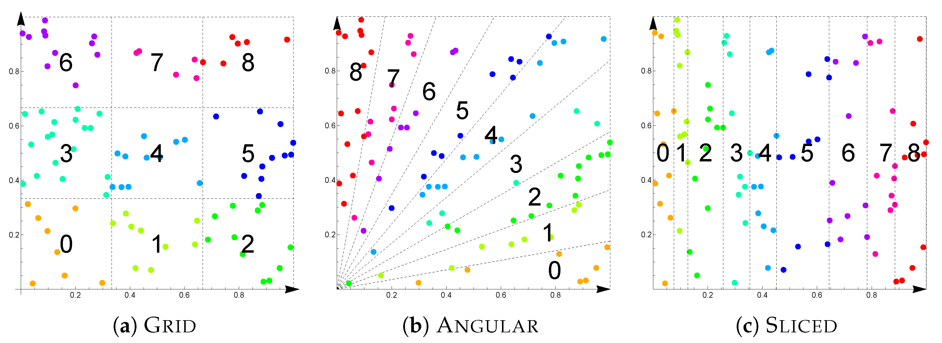
A common limitation of skyline queries is their complexity, generally quadratic in the dataset size, which poses challenges in big data contexts. To mitigate this, researchers have been exploring dataset partitioning strategies to enable parallel processing, thereby reducing the overall computation time. A common application scenario, which is the one used here, regards the so-called horizontal partitioning, in which each partition is assigned a subset of the tuples. Peer-to-peer (P2P) architectures [2] first explored this approach, by having each peer to compute its skyline locally and then merging it with the rest of the network. The typical approach, indeed, involves a two-phase process: the first involves computing local skylines within each partition; the second involves merging these local skylines to create a pruned dataset for the final skyline computation. The aim is to eliminate as many dominated alternatives as possible during the local skyline phase, minimizing the dataset size for the final computation. With the maturity of parallel computation paradigms such as Map-Reduce and Spark and the usage of GPUs, parallel solutions reflecting this pattern have become common [3,4,5] and have been subjected to careful experimental scrutiny [6].

Another limitation of skylines as a query tool is that they may return result sets that are too large and thus of little use to the final user. A way around this problem is to equip skyline tuples with additional numeric indicators that measure their “strength” according to various characteristics. With this, skyline tuples can be ranked and selected accordingly to offer a more concise result to the final user. Several previous research attempts, including [7,8,9,10,11,12,13,14,15,16,17,18,19,20], have proposed a plethora of such indicators. We focus here on an indicator, called the grid resistance [20], that measures how robust a skyline tuple is to slight perturbations of its attribute values. Quantizing tuple values (e.g., in a grid) affects dominance, since, as the quantization step size grows, more values tend to collapse, causing new dominance relationships to occur.

The computation of this indicator may involve, in turn, several rounds of computation of the skyline or of the dominance relationships. In this respect, the parallelization techniques that have been developed for the computation of skylines may prove especially useful for the indicators too. In this work, we describe the main parallelization opportunities for the computation of the grid resistance of skyline tuples and provide an experimental evaluation that analyzes the impact of such techniques in several practical scenarios.

The grid resistance indicator was only proposed very recently [20], and no prior algorithmic study exists that has detailed the steps necessary to compute the result, particularly in a parallelized setting. The solution presented here goes beyond the sketchy sequential pattern given in [20] and, building on consolidated research on data partitioning in skyline settings, offers the first attempt to parallelize the computation of grid resistance. In fact, to the best of our knowledge, this is also the first attempt to adapt the parallelization strategies used for skylines to compute other notions.

2. Materials and Methods

The main algorithmic patterns used in this paper are described in detail in Section 4. The data and computer code used in the experiments are available upon request to the author.

In particular, the datasets used for the experiments comprise both synthetic and real datasets. For the synthetic datasets, we produce, for several combinations of the size N and number of dimensions d, three d-dimensional datasets of size N with values in the $[0,1)$ interval: one with values anti-correlated across different dimensions ($\mathtt{ANT}$); one with uniformly distributed values ($\mathtt{UNI}$); and one with correlated values ($\mathtt{COR}$). For each dataset, we generate 5 different instances; our results reflect averages over these instances. More details on the synthetic datasets can be found in Section 5.

The real datasets that we adopt are the result of a cleaning, normalization, and attribute selection process that resulted in the following:

• $\mathtt{NBA}$—all-time stats for 4832 NBA players from nba.com as of 3 October 2023, from which we retained 2 attributes;
• $\mathtt{HOU}$—127,931 6D tuples regarding household data scraped from www.ipums.org (accessed on 3 December 2024);
• $\mathtt{EMP}$—291,825 6D tuples about City employees in San Francisco [21];
• $\mathtt{RES}$—real estate data from zillow.com (accessed on 3 December 2024), with 3,569,678 6D tuples;
• $\mathtt{SEN}$—sensor data with 7 numeric attributes and 2,049,280 tuples [22].

3. Preliminaries

We refer to datasets consisting of numeric attributes. Without loss of generality, the domain that we consider is the set of non-negative real numbers ${\mathbb{R}}^{+}$. A schema S is a set of attributes $\{A_1,\dots ,A_d\}$, and a tuple $t=\langle v_1,\dots ,v_d\rangle$ over S is a function associating each attribute $A_i\in S$ with a value $v_i$, also denoted as $t\left[A_i\right]$, in ${\mathbb{R}}^{+}$; a relation over S is a set of tuples over S.

A skyline query [1] takes a relation r as input and returns the set of tuples in r that are dominated by no other tuples in r, where dominance is defined as follows.

Definition 1. 

Let t and s be tuples over a schema S; t dominates s, denoted $t\prec s$, if, for every attribute $A\in S$, $t\left[A\right]\le s\left[A\right]$ holds and there exists an attribute $A^{\prime }\in S$ such that $t\left[A^{\prime }\right]<s\left[A^{\prime }\right]$ holds. The skyline Sky(r) of a relation r over S is the set $\{t\in r\mid \nexists s\in r.s\prec t\}$.

We shall consider attributes such as “cost”, where smaller values are preferable; however, the opposite convention would also be possible.

A tuple can be associated with a numeric score via a scoring function applied to the tuple’s attribute values. For a tuple t over a schema $S=\{A_1,\dots ,A_d\}$, a scoring function f returns a score $f(t\left[A_1\right],\dots ,t\left[A_d\right])\in {\mathbb{R}}^{+}$, also indicated as $f\left(t\right)$. As for attribute values, we set our preference for lower scores (but the opposite convention would also be possible).

Although skyline tuples are unranked, they can be associated with extra numeric values by computing appropriate indicators and ranked accordingly. To this end, we consider a robustness indicator.

The indicator called grid resistance, denoted as $\mathsf{gres}(t;r)$, measures how robust skyline tuple t is with respect to a perturbation of the attribute values of the tuples in r, i.e., whether t would remain in the skyline. In [20], this is achieved by restricting the tuple values to a grid divided into g equally sized intervals in each dimension: the more a skyline tuple resists larger intervals, the more robust it is. The grid projection $\mathsf{gproj}(t,g)$ of t on the grid is defined as $\mathsf{gproj}(t,g)=〈{\displaystyle \frac{\lfloor t\left[1\right]·g\rfloor }{g}},\dots ,{\displaystyle \frac{\lfloor t\left[d\right]·g\rfloor }{g}}〉,$ and this corresponds to the lowest-value corner of the cell that contains t. When tuples are mapped to their grid projections, we obtain a new relation $\mathsf{gproj}(r,g)=\left\{\mathsf{gproj}\right(t,g)\mid t\in r\}$, in which new dominance relationships may occur. The grid resistance $\mathsf{gres}(t;r)$ of t is the smallest value of $g^{-1}$ for which t is no longer in the skyline.

Definition 2. 

Let r be a relation and $t\in$ Sky(r). The grid resistance $\mathsf{gres}(t;r)$ of t in r is $\underset{g\in {\mathbb{N}}^{+}}{min}\{g^{-1}\mid \mathsf{gproj}(t,g)\notin$ Sky$\left(\mathsf{gproj}(r,g)\right)\}$. We set $\mathsf{gres}(t;r)=1$ if t never exits the skyline.

4. Parallel Algorithms

In this section, we first present the main partitioning strategies adopted in the literature and then describe how they can be adapted for the computation of the indicators.

Such strategies have been developed assuming a general scheme for the parallelization of the computation of the skyline that consists of the following phases:

• each partition is processed independently and in parallel to produce a “local” skyline; the union of these local skylines may still contain tuples that are dominated by tuples in other partitions;
• the final result is obtained by applying the skyline operator to the union of all the local skylines by removing all residual dominated tuples.

The input to the first phase may also include additional meta-information that will accelerate the process. The last phase is typically executed sequentially, but there are ways to parallelize this phase too [6].

4.1. Partitioning Strategies

We now review three of the main partitioning strategies available in the literature: grid partitioning, angle-based partitioning, and sliced partitioning.

Figure 1 illustrates the different partitioning strategies as applied to a uniformly distributed dataset of 90 tuples with 9 partitions, where different partitions are represented with different colors.

Grid partitioning [3] (Grid) partitions the space into a grid of equally sized cells, resulting in a total of $p=m^d$ partitions, where d denotes the total number of dimensions and m the number of slices in which each dimension is split. This strategy additionally entails a dominance relationship applied to grid cells (and thus to partitions), which allows us to avoid processing certain partitions completely.

We identify a given cell $c_i$ with its grid coordinates, $\langle c_i\left[1\right],\dots ,c_i\left[d\right]\rangle$, with $1\le c_i\left[j\right]\le m$, $j=1,\dots ,d$. With this, we can introduce grid dominance.

Definition 3 

(Grid dominance). For grid cells $c_i$ and $c_h$, $c_i$ grid-dominates $c_h$, denoted $c_i{\prec }_G{c}_h$, if, for every dimension j, $j=1,\dots ,d$, we have $c_i\left[j\right]<c_h\left[j\right]$.

If $c_i$ grid-dominates $c_h$, then all tuples in $c_i$ dominate all tuples in $c_j$, so, if $c_i$ is not empty, $c_j$ can be disregarded altogether when computing the skyline.

Assigning a partition number, shown in Figure 1a for grid partitioning, to a tuple t can be performed as follows, assuming, for simplicity, all values to be in $[0,1)$:

$$p\left(t\right)=\sum _{i=1}^d\lfloor t\left[A_i\right]·m\rfloor ·m^{i-1}$$

where $A_i$ is the i-th attribute. As an example of grid dominance that can be seen in the figure, partition 1 grid-dominates partitions 5 and 8.

Angle-based partitioning [23] (henceforth, Angular) partitions the space with regard to angular coordinates, after converting Cartesian to hyper-spherical coordinates, which provides a better workload balance across partitions than with Grid.

The partition number (shown in Figure 1b for Angular) is computed for every tuple t based on hyper-spherical coordinates, including a radial coordinate r and $d-1$ angular coordinates ${\phi }_1,\dots ,{\phi }_{d-1}$, obtained through standard geometric considerations from the Cartesian coordinates. The partition number of t is then computed as follows:

$$p\left(t\right)=\sum _{i=1}^{d-1}⌊{\displaystyle \frac{2{\phi }_i}{\pi }}m⌋m^{i-1}$$

(1)

where m is, again, the number of slices into which each (angular) dimension is divided, which essentially amounts to grid partitioning on angular coordinates.

Sliced partitioning [6] (Sliced) first sorts the dataset with respect to one chosen dimension and then (unlike Grid and Angular) determines any given number p of equi-numerous partitions. The partition number (shown in Figure 1c for Sliced) of the i-th tuple t in the ordering is simply computed as follows:

$$p\left(t\right)=⌊{\displaystyle \frac{(i-1)·p}{N}}⌋,$$

where N is the number of tuples in the dataset.

We observe that all the partitioning strategies can be improved by resorting to several optimization opportunities. We reconsider here the so-called representative filtering, as presented in [6]. Representative filtering consists of pre-computing a few potentially “strong” tuples to be shared across all partitions, since they may have strong potential to dominate other tuples, thus further removing redundant tuples in the local skylines of each partition. A simple technique to select representative tuples consists of choosing the top-k results according to any given monotone scoring function f of the dataset’s attributes. This can be achieved, e.g., in $\mathcal{O}(Nlogk)$, by using a (max-)heap as follows:

(i)

insert the first k tuples in the heap;

(ii)

scan the rest of the dataset and, for each tuple t, if $f\left(t\right)<f\left(t_k\right)$ (where $t_k$ is the tuple at the root of the heap), replace $t_k$ with t and re-adjust (heapify) the heap.

One can even obtain the same result in $\mathcal{O}(N+klogk)$ by

(i)

executing a selection algorithm running in $\mathcal{O}\left(N\right)$ to find the k-th smallest tuple according to f;

(ii)

using this as a pivot in the QuickSort sense to separate the k smallest tuples from the others; and

(iii)

finally sorting the k tuples in $\mathcal{O}(klogk)$.

See, e.g., [24] for details about the selection algorithm. Note that, after selecting the k representatives, those that are dominated by other representatives should be discarded, since they do not add any pruning power to the set; this means that the actual number of tuples used for the subsequent filtering is potentially lower than k.

4.2. Computing the Indicator

Finding $\mathsf{gres}$ requires recomputing the dominance on grid-projected datasets for various values of the grid interval g. Luckily, the $\mathsf{gres}$ operator is stable, i.e., it does not depend on dominated tuples, and therefore we can focus on skyline tuples alone. Algorithm 1 shows the pseudo-code illustrating this idea. The grid interval varies between 2 (smallest meaningful value) and an upper bound $\overline{g}$ that depends on the dataset. In particular, we have the guarantee that no new dominance relationship may occur when $g>\overline{g}=\lfloor {\ell }^{-1}\rfloor$, where ℓ is the absolute value of the smallest non-zero difference on the same attribute between any two tuples (line 2). It suffices then to compute, for each value of g among $\overline{g},\overline{g}-1,\dots ,2$ (line 3), the skyline Sky$\left(\mathsf{gproj}\right(r,g\left)\right)$ (line 4) and, for each tuple $t\in$ Sky(r), to test whether $\mathsf{gproj}(t,g)\in$ Sky$\left(\mathsf{gproj}\right(r,g\left)\right)$; the inverse of the first value of g for which membership does not hold is $\mathsf{gres}(t,r)$ (lines 5–6). If we ignore the dependence on $\overline{g}$, which is dataset-dependent, the complexity of computing $\mathsf{gres}$ for a given tuple is $\mathcal{O}\left(S^2\right)$, where S = |Sky(r)| $\in \mathcal{O}\left(N\right)$, i.e., in the worst case, $\mathcal{O}\left(N^2\right)$. It is strikingly evident that computing $\mathsf{gres}$ requires several rounds of computation of the skyline (although on a potentially much smaller dataset than the starting one, since dominated tuples can be disregarded completely). In this respect, adopting the partitioning strategies that typically quicken skyline computation may be beneficial for $\mathsf{gres}$ too.

Algorithm 1: Algorithmic pattern for computation of $\mathsf{gres}$

Input:       skyline $s=$ Sky(r) Output:       a map from every tuple $t\in s$ to $\mathsf{gres}(t,r)$ 1.     $map:=\varnothing$ // the result map, initially empty 2.     $\overline{g}:=\lfloor {\ell }^{-1}\rfloor$ // where ℓ is the minimum possible value for $\mathsf{gres}$ 3.     for each  g  in  $\overline{g},\overline{g}-1,\dots ,3,2$  do 4.        $s^{\prime }:=$ Sky$\left(\mathsf{gproj}(r,g)\right)$ 5.        for each t in s do 6.           if $\mathsf{gproj}(t,g)\notin s^{\prime }\wedge map\left(t\right)=\mathbf{nil}$ then $map\left(t\right):=g^{-1}$ 7.     for each  t  in  s  do 8.        if $map\left(t\right)=\mathbf{nil}$ then $map\left(t\right):=1$ // t never exited the skyline 9.     return $map$

5. Results

In this section, we test the effectiveness and efficiency of the proposed algorithmic pattern (Algorithm 1) on a number of scenarios covering a wide range of representative cases of datasets with diverse characteristics, such as size, dimensionality, and value distribution. For better representativeness, our selection of datasets comprises three synthetic datasets (ANT, UNI, and COR) and five real datasets ($\mathtt{NBA}$, $\mathtt{HOU}$, $\mathtt{EMP}$, $\mathtt{RES}$, and $\mathtt{SEN}$), as described in Section 2. Such a wide and diversified choice increases the robustness of our experimental campaign and helps to reveal general trends and corner cases in our analysis.

In our experiments, we vary several parameters (shown in

Table 1. Operating parameters for testing of efficiency (defaults in bold).

Full Name	Tested Value
Distribution	synthetic: ANT, UNI; real: NBA, HOU, EMP, RES, SEN
Synthetic dataset size (N)	100 K, 500 K, 1 M, 5 M, 10 M
# of dimensions (d)	2, 3, 4, 5, 6, 7
# of partitions (p)	16, 32, 64, 128
# of representatives ($rep$)	0, 1, 10, 100, 1000
# of cores (c)	2, 4, 8, 16

) to measure their impacts, on various datasets, on the number of dominance tests required to compute the final result:

• the dataset cardinality N;
• the number of dimensions d; and
• the number of partitions p.

Since, with Grid and Angular, not all values of p are possible, we run them with a value of p that is closest to the target number shown in Table 1, provided that the number of resulting partitions is greater than 1.

The number of dominance tests incurred during the various phases of our algorithmic patterns provides us with an objective measure of the effort required to compute the indicators, independently of the underlying hardware configuration.

Any computing infrastructure will essentially face (i) an overhead for the parallel phase, (ii) one for the sequential phase, and (iii) one for the orchestration of the execution and communication between nodes. While (iii) depends on the particular infrastructure, (i) and (ii) will depend directly on the number of dominance tests. In particular, the cost of the sequential phase will be proportional to the number of dominance tests performed during that phase, while, in the parallel phase, the cost will be proportional to the largest amount of dominance tests that need to be pipelined by the parallel computation. In short, if there is at least one core per partition, the parallel phase will roughly cost as much as the processing cost incurred by the heaviest partition; if the partition/core ratio is k, then the cost of the parallel phase will be scaled by a factor k.

Besides the objective measure given by the dominance tests, we also measure the execution times by parallelizing the tasks on a single MacBook Pro machine with an Apple M4 chip with a 16-core CPU, 48GB of unified memory, and 1TB SSD storage, running MacOS Sequoia 15.2. Our implementation of the algorithmic pattern shown in Algorithm 1 was developed in the Swift 6.0 programming language, which, through its Automatic Reference Counting policy, guarantees a very low memory profile during the execution. The parallelization of the execution is achieved by orchestrating the process through the Grand Central Dispatch (GCD) adopted by Swift and controlling the number of active cores through semaphores, while eventually notifying a coordinator when all the parallel (local skyline computation) tasks are completed. In particular, a dispatch group (DispatchGroup) is used to track the completion of asynchronous tasks; a concurrent queue (DispatchQueue) receives the execution of the asynchronous tasks; and a semaphore (DispatchSemaphore) limits the number of concurrent tasks to the desired amount. The coordinator loops through the pending tasks and, for each task, waits for an available core using the semaphore, enters the dispatch group, and requests the asynchronous execution of the task. At the end of the execution, we signal the semaphore to release a core and leave the dispatch group. Finally, at the end of the loop, the coordinator is notified on the main queue.

We now report our experiments on the computation of $\mathsf{gres}$ with the different partitioning strategies. Before starting the experiments, we observe that, while the exact determination of $\mathsf{gres}$ would require determining ℓ as in line 2 of Algorithm 1 and its inverse $\overline{g}$, the actual value of ℓ may be impractically small. Bearing in mind that the aim of the $\mathsf{gres}$ indicator is to determine the tuples that are “strong” with regard to grid resistance, and that, for very small values of ℓ, the corresponding value of $\mathsf{gres}$ would be insignificant, we choose to move to a more practical option. Therefore, instead of looking for the smallest non-zero difference (in absolute value) between any two values on the same attribute in the dataset, we simply set $\overline{g}=25$ as a reasonable threshold of significance for the number of grid intervals.

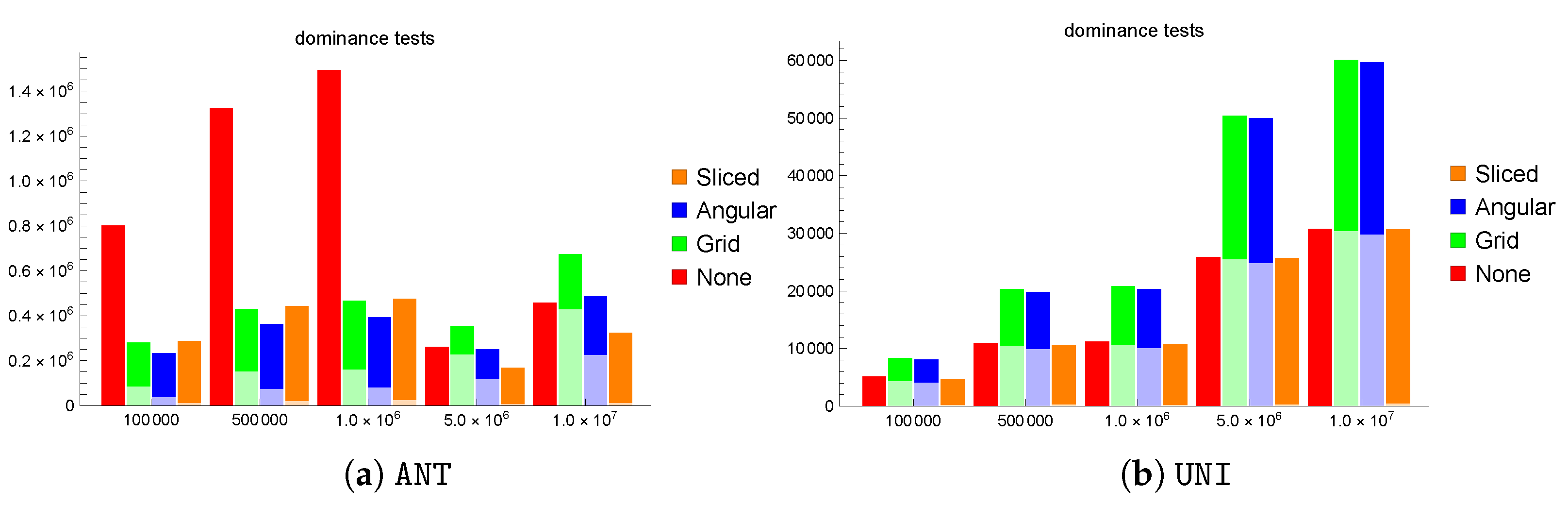
Varying the dataset size $\mathit{N}$. Our first experiment focuses on the effect of the dataset size on the number of dominance tests needed to compute the result, while keeping all the other operating parameters to their default values, as indicated in Table 1. Figure 2a focuses on ANT and reports stacked bars for each of the partitioning strategies, in which the lower part refers to the largest number of dominance tests performed in any partition during the parallel phase, while the top part indicates the number of dominance tests performed during the final phase. We observe that, up to $N=1$ M, all partitioning strategies are beneficial with respect to no partitioning (indicated as None), with Angular as the most effective strategy and Sliced as the strategy with the lowest parallel costs, due to the ideal balancing of the number of tuples in each partition. For larger sizes, however, Grid becomes less effective, Angular is on par with None, and Sliced becomes the most effective strategy. This is due to the non-monotonic behavior with respect to the number of skyline points: for a growing dataset size, the size of the skyline typically also grows; however, when we move from $N=1$ M to $N=5$ M, there is a fall from 1022 to only 527 tuples in |Sky|. This is due to the fact that the larger dataset, besides containing more tuples, also includes some very strong tuples that dominate most of the remaining ones. A similar effect is observed for $N=10$ M, for which the skyline size only grows to 650 tuples and is therefore smaller than with $N=1$ M and actually even smaller than with $N=500$ K (where |Sky|$=940$) $N=100$ K (where |Sky|$=719$). These numbers refer to one of our exemplar instances, but similar behaviors, which are due to the way in which the data are generated (we adopted the widely used synthetic data generator proposed by the authors of [1]), are nonetheless common to all five repetitions of the experiments that we describe.

Figure 2b shows the stacked bars for the UNI dataset. Here, the benefits of parallelization are essentially lost, at least for Grid and Angular, due to the extremely small skyline sizes that occur with uniform distributions (varying from 75 tuples for $N=100$ K to 101 for $N=10$ M). The Sliced partitioning strategy manages to still offer slight improvements with respect to None by performing very little removal work during the parallel phase; therefore, the final phase is only slightly lighter than with None.

An even more extreme situation occurs with the COR dataset, for which the skyline sizes are so small that the benefits of parallelism are completely nullified. For instance, with default parameter values ($N=1$ M and $d=3$), the skyline barely consists of two tuples and the computation essentially amounts to 25 dominance tests, i.e., one per tested grid interval value. The situation does not change for other values of N, with $\left|sky\right|$ always less than 5. For this reason, we refrain from considering the COR dataset further.

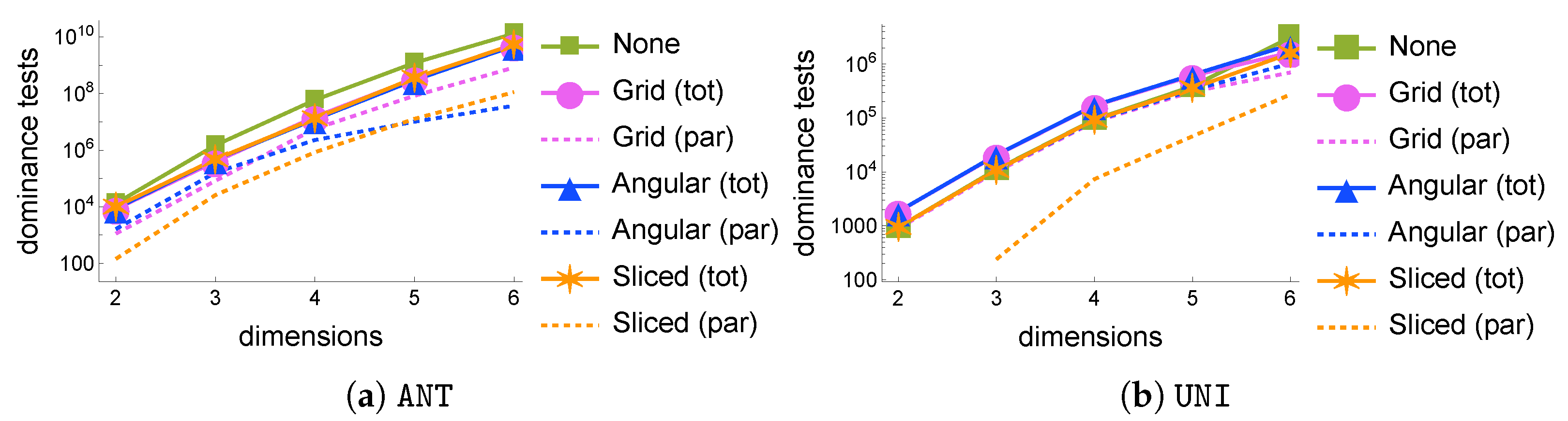
Varying the number of dimensions $\mathit{d}$. Figure 3 shows how the number of dominance tests varies as the number of dimensions in the synthetic dataset grows. The plots need to use a logarithmic scale since the number of tests grows exponentially, as an effect of the “curse of dimensionality”. With the ANT datasets (Figure 3a), all partitioning strategies offer significant gains with respect to the plain sequential execution, with savings of up to nearly 80% and never under 60% for $d>2$. Indeed, when $d=2$, the skyline consists of only 62 tuples, so the benefits of partitioning are smaller. In particular, Grid is the top performer for $d\le 4$, while Angular wins for $d\ge 5$, although the differences between the best and the worst strategies are always under 5%. The dashed lines indicate the largest number of dominance tests performed in any partition during the parallel phase, while the solid lines indicate the overall cost of a parallel execution, i.e., by adding to the previous component the number of dominance tests in the final phase.

In the case of UNI datasets, the skyline sizes are very small for low d, with as few as 11 tuples when $d=2$. Clearly, parallelizing does not yield benefits in such circumstances. For larger values of d, the gains are more significant, reaching nearly 50% when $d=6$ with the Sliced strategy, which proves to be the most suitable for this type of dataset in all scenarios, while Grid and Angular reach 26% and 47%, respectively, under the same conditions. We also note that, when there are more partitions than skyline points (as is the case, e.g., with $d=2$, in which $p=16>11=$ |Sky|), the partitions in Sliced will have either 0 or 1 points, so no dominance test will ever take place in the parallel phase, which is then completely ineffective.

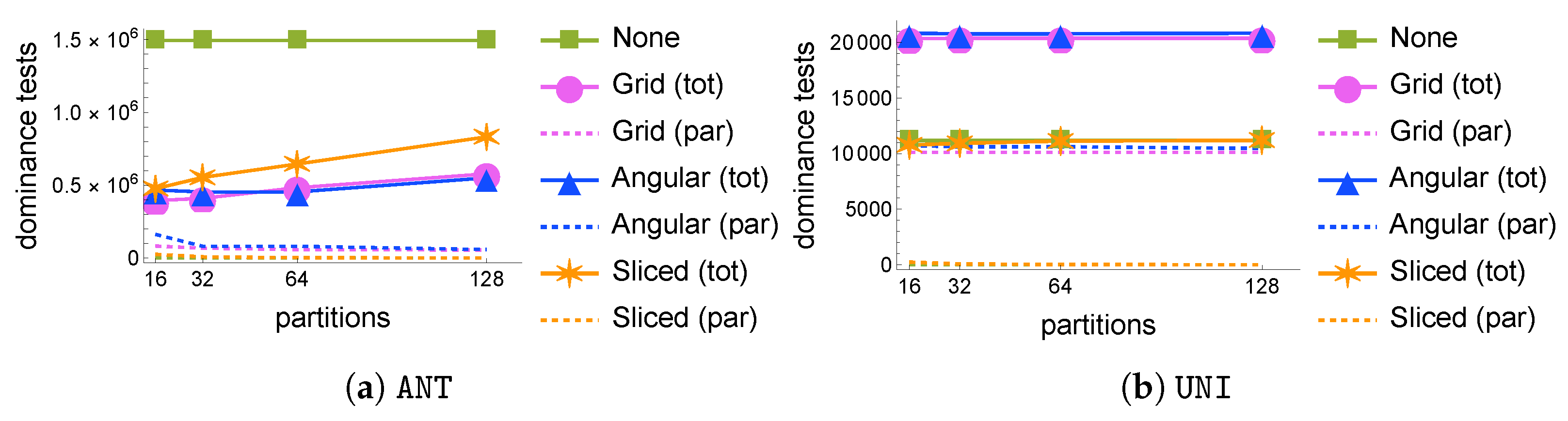
Varying the number of partitions $\mathit{p}$. Figure 4 shows the effect of the number of partitions on the number of dominance tests. While the partitioning is always beneficial with the ANT datasets (Figure 4a), increasing the number of partitions only increases the overhead. This phenomenon is due to two factors: the first one is the relatively small size of the input dataset for the computation of $\mathsf{gres}$, i.e., the size of the skyline of a 3D dataset of 1 M tuples (1022 tuples in our case), which makes it less open to more intense parallelization opportunities; the second reason is that, since the input consists of skyline tuples of the original dataset, for small grid intervals (i.e., for larger values of g as used in Algorithm 1), the grid projections of these skyline tuples will almost never exit the skyline, so that dominance tests will be ineffective and the final phase will be predominant, as can be clearly seen, e.g., in Figure 4b. For UNI, these effects do not change but are less visible because of the much smaller skyline size involved (just 78 tuples), which makes Grid and Angular completely ineffective, while Sliced maintains performance on par with or slightly better than that of None.

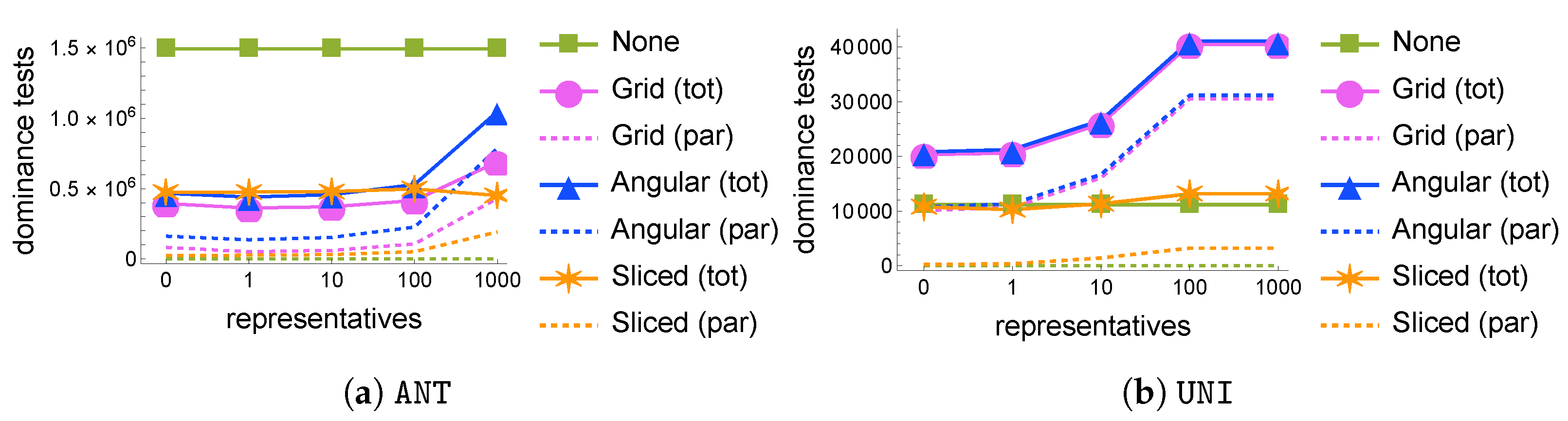
Varying the number of representatives $\mathit{rep}$. We now measure the effects of the representative filtering technique on the computation of $\mathsf{gres}$ by varying the number of representative tuples, $rep$, with default values for all other parameters for synthetic datasets. Figure 5 clearly shows that representative filtering is overall ineffective: in almost all considered scenarios, using representatives only overburdens the parallel phase with additional dominance tests, without actually significantly reducing the union of local skylines. Again, this is due to the fact that grid projections of skyline points are very likely to remain non-dominated, especially for smaller grid sizes, so that the pruning power of representative tuples fades. The only case where a small advantage emerges is with Sliced on ANT with $rep=1000$, which determines a minor 5% decrease in the number of dominance tests with respect to the case with no representatives. We also observe that a target number of representatives corresponds to a smaller average number of actually non-dominated tuples; for instance, on ANT, only $3.88$ tuples are non-dominated, on average, out of 10 selected representatives, and only $132.36$ out of 1000.

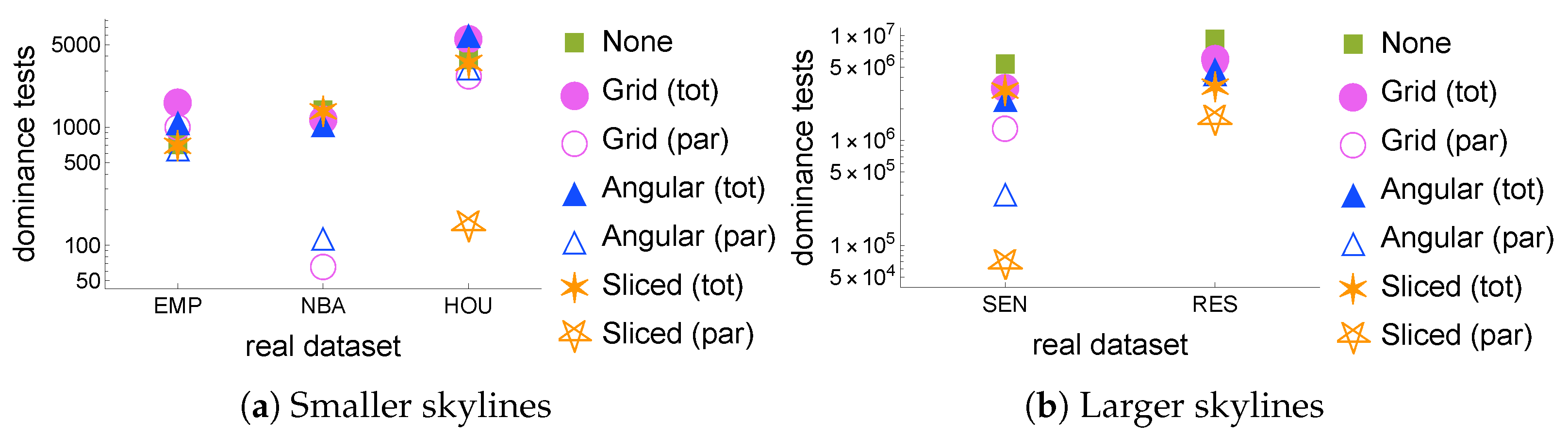
Real datasets. Figure 6 shows how the number of dominance tests varies depending on the partitioning strategy on different real datasets. Figure 6a shows the three datasets with smaller skyline sizes, EMP, NBA, and HOU, whose skyline sizes are, respectively, 14, 14, and 16. Note that, while $\mathtt{NBA}$ is a small dataset, the other two are much larger, but their tuples are correlated, thus causing a smaller skyline. Figure 6b shows what happens with real datasets with larger skylines: SEN has 1496 tuples in its skyline, while $\mathtt{RES}$ has 8789. The results shown in the figure confirm what was found in the synthetic datasets: for the smaller cases, Angular and Grid do not yield benefits, while Sliced essentially has no parallel phase, thereby coinciding with or slightly improving over None. With the larger datasets, the gains are at least 35% with all strategies on SEN and at least 29% on RES, with peak improvements of 50% on SEN by Angular and 64% on RES by Sliced.

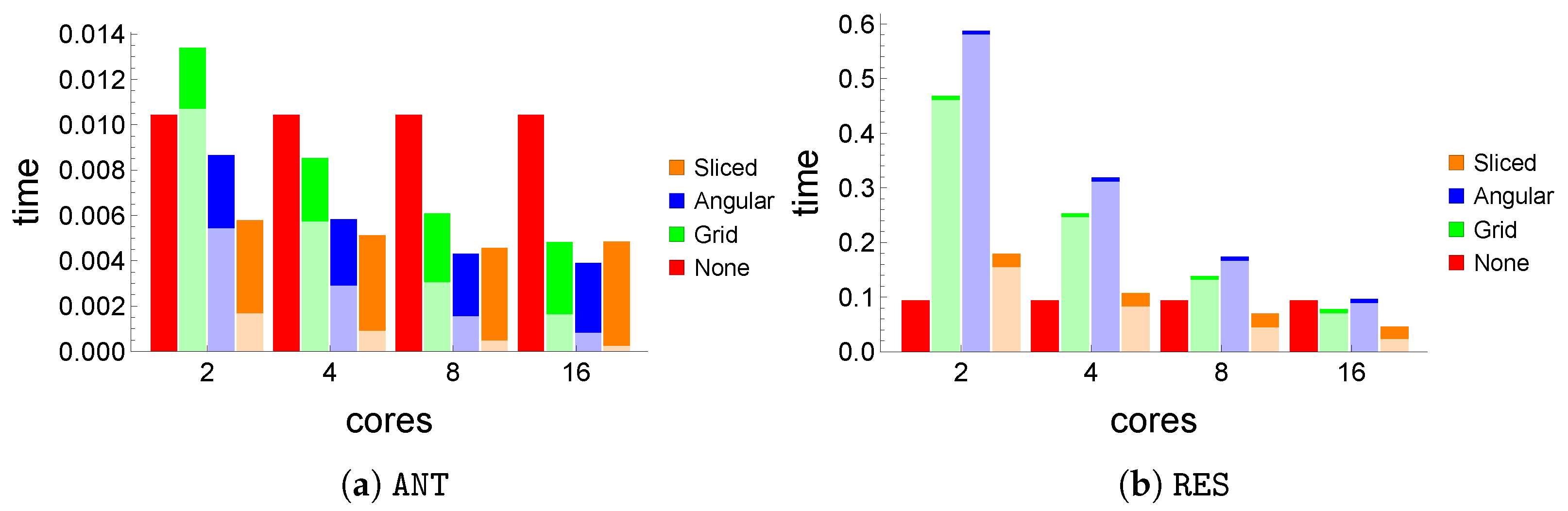
Execution times. In order to analyze the concrete execution time required to complete the computation of $\mathsf{gres}$ using the different partitioning strategies, we focus on ANT and RES, i.e., the most challenging synthetic and real datasets, respectively. Figure 7 shows stacked bars reporting the breakdown of the execution time for the various partitioning strategies with two components: the time needed to complete the parallel phase (the lower part of the bar, shown in a lighter color) and the rest of the time (the upper part), including the final, sequential phase and the additional overhead caused by the coordination of the execution over multiple cores. In our execution setting, computing $\mathsf{gres}$ for all the tuples in the skyline of ANT with the default parameter values (Figure 7a) requires $0.01$ s with a plain, sequential implementation, in which the skyline is computed through a standard SFS algorithm [25]. Parallelization starts to yield benefits with just two cores with Angular and Sliced, while it takes at least four cores for Grid to surpass None. With 16 cores, all strategies find the result in less than half the time required by None. We observe that, while all partitioning strategies improve as the number of cores grows, Sliced improves very little after eight cores, since its parallel phase, for this dataset, is already very light when compared to the final phase. Figure 7b shows similar bars for the RES dataset, but, here, due to the nature of the data, the times are approximately ten times higher ($0.1$ s for a plain sequential execution) and all parallel strategies incur high parallel costs, as shown in the lower parts of the bars. While more cores are needed to perceive tangible improvements, all strategies attain better performance than None with 16 cores, all still having a large part of their execution time taken by the parallel phase, i.e., showing potential for further improvements in their performance with the availability of more cores (with 16 cores, Sliced already requires less than half the time taken by None to compute the result).

Final observations. Our experiments show that the parallelization opportunities offered by the partitioning strategies analyzed are useful for the computation of $\mathsf{gres}$, provided that the application scenario is challenging enough to make the parallelization effort worthwhile, as we found to be the case with the ANT datasets and with real datasets such as RES and SEN. While there is no clear winner in all cases, Sliced provides the most stable performances across all datasets. The nature of the problem at hand, which involves many tuples that are already strong, being part of the initial skyline, makes the representative filtering optimization ineffective and does not suggest the use of an overly high number of partitions. While we conducted our analysis through the detailed counting of dominance tests, our results also indicate that a simple single-machine environment with 16 cores is sufficient to experience two-times improvements in the execution times in the most challenging datasets adopted for our experiments. The main limitations of our approach are tightly connected to the parallelizability of the problem at hand. This, in turn, requires a large enough initial skyline set so that the partitioning strategy can effectively divide the work into suitable chunks. This is only the case in uniformly distributed or smaller datasets and moderately so in the larger, real datasets that we have tested. A case in which our approach performs particularly poorly is that of datasets with correlated data: no savings are obtained in terms of dominance tests and the overall execution times are nearly one order of magnitude worse than without parallelization (although very small, in the order of $0.1$ ms), which brings its overhead with no gains. We observe, however, that the cases in which the parallelization of the computation of $\mathsf{gres}$ does not help are also those in which speed-ups are less needed and the times are already very small.

6. Related Work

In the last two and a half decades, the skyline operator has spurred numerous research efforts aiming to reduce its computational cost and augment its practicality by trying to overcome some of its most common limitations. While some of the essential works in this line of research have been presented already in Section 1, we now try to provide a more complete picture.

Skylines are the preference-agnostic counterpart of ranking (also known as top-k) queries; while the former offer a wide overview of a dataset, the latter are more efficient, provide control over the output size, and apply to a large variety of queries, including complex joins and all types of utility components in their scoring functions (i.e., the main tool for the specification of preferences) [26,27,28]. Recently, hybrid approaches have started to appear, trying to exploit the advantages of both [29,30].

As regards the efficiency aspects, several algorithms have been developed to address the centralized computation of skylines, including [1,25,31]. In order to address the most serious shortcomings of skylines, many different variants have been proposed so as to, e.g., accommodate user preferences and control or reduce the output size (which tends to grow uncontrollably in anti-correlated or highly dimensional data) or even add a probabilistic aspect to it; a non-exhaustive list of works in this direction is [30,32,33,34].

Improvements in efficiency have been studied also in the case of the data distribution. In particular, in addition to the horizontal partitioning strategies discussed here with the pattern described at the beginning of Section 4, vertical partitioning has been studied extensively in the seminal works of Fagin [35] and subsequent contributions, addressing the so-called middleware scenario.

While skyline tuples are part of the commonly accepted semantics of “potentially optimal” tuples of a dataset, in their standard version, they are returned to the final user as an unranked bunch. Recent attempts have been trying to counter this possibly overwhelming effect, which is particularly problematic in the case of very large skylines, by equipping skyline tuples with additional numeric scores that can be used to rank them and focus on a restricted set thereof. The first proposal was to rank skyline tuples based on the number of tuples that they dominate [8]; albeit very simple to understand, the subsequent literature has criticized this indicator for a number of reasons, including the fact that

(i)

it may be applied to non-skyline tuples too and thus the resulting ranking may not prioritize skyline tuples over non-skyline tuples;

(ii)

too many ties would occur in such a ranking; and

(iii)

it is not stable, i.e., it depends on the presence of “junk” (i.e., dominated) tuples.

Later attempts focused on other properties, including, e.g., the best rank that a tuple might have in any ranking obtainable by using a ranking query with a linear scoring function (i.e., the most common and possibly the only type of scoring function adopted in practice) [36]. More recently, with the intention of exposing the inherent limitations of linear scoring functions, the authors of [20] introduced a number of novel indicators to measure both the “robustness” of a skyline tuple and the “difficulty” in retrieving it with a top-k query. The indicators measuring difficulty are typically based on the construction of the convex hull of a dataset, whose parallel computation has been studied extensively [37,38,39]. Convex hull-based indicators include the mentioned best rank and the so-called concavity degree, i.e., the amount of non-linearity required in the scoring function for a tuple to become part of the top-k results of a query. As for robustness, the indicator called the exclusive volume refers to the measure of volume in the dominance region of a tuple that is not part of the dominance regions of any other tuples in the dataset; this indicator is computed as an instance of the so-called hypervolume contribution problem, which has also been studied extensively and is #P-hard to solve exactly [40,41]. Finally, grid resistance is the main indicator of robustness, which we thoroughly analyzed in this paper. The notion of stability [42] is akin to robustness in the sense that it still tries to measure how large perturbations can be tolerated to preserve the top-k tuples of a ranking, although the focus is on attribute values in the scoring function and not on tuple values, as is the case for grid resistance. To the best of our knowledge, apart from the sketchy sequential pattern given in the seminal paper [20], there is no prior work on the computation of the grid resistance, particularly in a parallelized setting.

We also observe that both skylines and ranking queries are commonly included as typical parts of complex data preparation pipelines for subsequent processing based, e.g., on machine learning or clustering algorithms [43,44]. In this respect, an approach similar to ours can be leveraged to improve the data preparation and to assess the robustness of the data collected by heterogeneous sources like RFID [45,46].

7. Conclusions

In this paper, we tackled the problem of assigning and computing a value of strength to skyline tuples, so that these tuples can be ranked and selected accordingly. In particular, we have focused on a specific indicator of robustness, called grid resistance, that measures the amount of value quantization that can be tolerated by a given skyline tuple for it to continue to be part of the skyline. Based on now consolidated algorithmic patterns that exploit data partitioning for the computation of skylines, we reviewed the main partitioning strategies that may be adopted in parallel environments (Grid, Angular, Sliced), as well as a common optimization strategy that can be used on top of this (representative filtering), and devised an algorithmic scheme that can be used to also compute the grid resistance on a partitioned dataset.

We conducted an extensive experimental evaluation on a number of different real and synthetic datasets and studied the effect of several parameters (dataset size, number of dimensions, data distribution, number of partitions, and number of representative tuples) on the number of dominance tests that are ultimately required to compute the grid resistance. Our results showed that all partitioning strategies may be beneficial, with Grid often reaching lower levels of effectiveness than Angular and Sliced. We have observed that the specific problem at hand, in which one only manages skyline (i.e., inherently strong) tuples, makes representative filtering ineffective and suggests to not over-partition the dataset. Indeed, the relatively low value that we used as the default for the number of partitions ($p=16$) also proved to be a good choice from a practical point of view. Our experiments on the execution time as the number of available cores varied confirmed the objective findings on the number of dominance tests and showed that, even with the limited parallelization opportunities offered by a single machine, the use of partitioning strategies may improve the performance by more than 50%, suggesting that there is room for further improvements with an increased number of available cores.

Our results also show the remarkable impact of the dataset characteristics (namely, the data distribution) on the performance. In particular, smaller or uniformly distributed datasets hardly benefit from the parallelized approach, since the problem size does not lend itself well to partitioning—an effect that is exacerbated in the case of correlated datasets. Anti-correlated datasets, according to our experiments, offer the most tangible improvements when exploiting partitioning.

While parallel processing does not lower the asymptotic computational complexity of the problem, which remains quadratic in the dataset size (and linear in the number of grid intervals to be tested, i.e., in the desired precision of the resulting grid resistance value), substantial gains can be experienced in practice, as we observed, in terms of both the overall dominance tests and the execution times.

No fair comparison with other approaches can be carried out at this time since, to the best of our knowledge, ours is the first parallel proposal for the computation of $\mathsf{gres}$. The sketchy sequential pattern described in [20] essentially corresponds to no partitioning (the None strategy), which has been thoroughly analyzed and extensively compared with our approach in Section 5.

Future work will try to adapt or revisit the techniques used in this paper to the computation of other notions that are built on top of dominance. These include, e.g., skyline variants, based on modified notions of dominance, as well as other indicators of the strength of skyline tuples, either novel or already proposed in the pertinent literature.