Inversion-Based Deblending in Common Midpoint Domain Using Time Domain High-Resolution Radon

Abstract

We implement an inversion-based deblending method in the common midpoint gathers (CMP) as an alternative to the standard common receiver gather (CRG) domain methods. The primary advantage of deblending in the CMP domain is that reflections from dipping layers are centred around zero offsets. As a result, CMP gathers exhibit a simpler structure compared to common receiver gathers (CRGs), where these reflections are apex-shifted. Consequently, we can employ a zero-offset hyperbolic Radon operator to process CMP gathers. This operator is a computationally more efficient alternative to the apex-shifted hyperbolic Radon required for processing CRG gathers. Sparse transforms, such as the Radon transform, can stack reflections and produce sparse models capable of separating blended sources. We utilize the Radon operator to develop an inversion-based deblending framework that incorporates a sparse model constraint. The inclusion of a sparsity constraint in the inversion process enhances the focusing of the transform and improves data recovery. Inversion-based deblending enables us to account for all observed data by incorporating the blending operator into the cost function. Our synthetic and field data examples demonstrate that inversion-based deblending in the CMP domain can effectively separate blended sources.

1. Introduction

The quest for efficient seismic data acquisition is a well-known challenge in geophysical exploration. Simultaneous acquisition, also known as blended acquisition, stands as a solution, offering a method that significantly reduces the time spent in the field by concurrently firing multiple sources. This technique, which was initially proposed by Garottu [1] for vibroseis acquisition and later expanded by Beasley et al. [2], Beasley [3] for marine environments, allows for the interference of sources at acquisition time which are subsequently separated during processing. Despite its time-saving advantages, existing models and algorithms for deblending such data often come with limitations.

This study is motivated by the need to address these limitations and to enhance the accuracy and efficiency of seismic data deblending. Current methods, including random firing and phase encoding, have paved the way for approaches to data acquisition. However, the deblending process remains a significant bottleneck, with two predominant schools of thought: the denoising-based approach [4], which focuses on erratic and random noise attenuation, and the inversion-based approach [5], which seeks to reconstruct the signal by inverting the blending process. This paper will mainly focus on processing data from the random firing approach.

The introduction of small random delays to the source firing times, as suggested by Berkhout [6], is a critical step in the deblending process. Pseudo-deblending involves remapping the blended shots to zero firing time and duplicating frames according to the number of simultaneous sources. This manipulation due to the random delays renders the interference from neighbouring sources as random noise in some of the common data domains, leaving only the target signal for recovery as coherent events. Pseudo-deblended data then show incoherent structures within the common midpoint gather (CMP), common receiver gather (CRG), and common offset gather (COF) domains, thus facilitating the deblending process. There are various methods to exploit the incoherency of blending noise, such as the separation work by Lin and Herrmann [7] and subsequent techniques such as Stolt Radon denoising [8], SSA filtering [9], denoising using a space-varying median filter [10], preconditioning with a discrete curvelet filter [11], and preconditioning with robust thresholding in the FK domain [12], each with their own advantages and drawbacks, often struggling with either issues in effectively distinguishing between signal and noise (source interference) for the denoising approaches or highly expensive and complex transform operators for the inversion-based approaches.

This paper introduces an inversion-based deblending approach utilizing the CMP domain, which promises a high-speed solution using a Radon transform operator. The utilization of the hyperbolic Radon transform for deblending serves multiple functions and significantly aids in the recovery of the seismic signal. Given the intrinsic nature of seismic acquisition, the acoustic responses emanating from the Earth’s interior manifest as hyperbolic arrivals at the surface. The hyperbolic Radon transform, by aggregating data based on hyperbolic trajectories, is ideally suited for mapping seismic data. Opting for the CMP domain over the traditional CRG domain method allows for the employment of a more streamlined version of the Radon transform operator, resulting in reduced runtimes.

2. Theory

2.1. Blending Operator

The blending operator allows us to transition between the blended domain, where sources are overlapped, referred to as a super shot, to the unblended domain, where sources belong to their respective shot records with firing times adjusted to zero for each shot. This can be represented as the blending operator $\mathbf{\Gamma }$, which contains the overlap and delay time information. We can then represent our unblended data cube as $\mathbf{D}$ and our blended data as $\mathbf{b}$ with the following relationship [6,13]:

$$\mathbf{b}=\mathbf{\Gamma }\mathbf{D}.$$

(1)

Applying the adjoint of the blending operator to the blended data, we obtain the pseudo-deblended data, in the unblended space, with each shot occupying its own data frame as opposed to multiple shots per data frame. This can be expressed by the following [6,13]:

$$\tilde{\mathbf{D}}={\mathbf{\Gamma }}^{\mathbf{H}}\mathbf{b}.$$

(2)

Here, $\tilde{\mathbf{D}}$ represents the pseudo-deblended data in standard shot frames. The blending matrix’s role is to amalgamate shots with random delay times, effectively superimposing individual shot record data. This also means that pseudo-deblending acts to redistribute the data to their respective frames. This forms an overcomplete representation of the data with redundant information stored in each pseudo-blended source panel. It is important to note that the adjoint operator does not eliminate source interference from the data; it merely copies it around.

The successful deblending of data using the random firing technique hinges on the inclusion of random delay times. These delays are critical in converting source interferences into what resembles random noise when remapping the data via the adjoint blending operator. It is essential that these delay times are sufficiently randomized to the point that no patterns emerge in the remapped data domains, as coherent patterns in the delay times reduce the effectiveness of our coherency constraint. Furthermore, the delays should be sufficiently long to ensure the separability of events, adhering to the minimum delay length determined by a function of the lowest frequency and blending fold, as detailed in Jiang and Abma [14]. Concurrently, they must be short enough that we gain an advantage in reduced acquisition times.

Random delays introduced into the blending schedule, and consequently the blending operator, are crucial for simplifying deblending. When the adjoint blending operator (pseudo-deblending) is applied to the blended dataset, the random delays become pivotal. Blending can be conceptualized as an operation on standard acquisition data that introduces source interference.

The influence of the addition on the random delay times can be seen when data are sorted into one of the other geometric domains after pseudo-deblending. After the application of the adjoint blending operator, coherent events can be seen in addition to the incoherent ones seen before the transform is applied; these coherent events are what we aim to extract, as they represent the part of the data that have their delay times properly corrected for, with the spontaneous data due to interfering shots that need to be removed. Through the use of an inversion method and a coherency constraint such as the high-resolution Radon transform, we can effectively remove the interfering signal and deblend our data.

2.2. Radon Transform

To solve the underdetermined issue seen in the inversion problem, we utilize the hyperbolic Radon transform (HRT) to further constrain the problem. This composite operator, which is made up of both the blending operator and the Radon transform operator, now reformulates the inversion into a sparsely constrained problem. The HRT is a variant of the Radon transform that sums across hyperbolic basis functions; in geophysics, this equation is defined as a function of arrival times and source–receiver offset and interval velocity, as seen in Thorson and Claerbout [15]:

$$m(p,\tau )={\int }_{h_1}^{h_2}d(h,t=\sqrt{{\tau }^2+p^2{h}^2})dh.$$

(3)

Here, $m(p,\tau )$ represents the Radon space data, p denotes the slowness, $\tau$ is the two-way travel time, h1 and h2 are the lower and upper offset limits, respectively, and d is the data space to be transformed. The slowness p is defined as the inverse of velocity $1/v$. Mapping based on hyperbolic arrivals allows for a precise and sparse representation of seismic data as seismic signals show up as hyperbolic events on standard seismic surveys. The Radon transform has been employed in various applications, including velocity analysis [15], multiple suppression [16], interpolation in the frequency or time domain [17], and deblending via denoising [8].

Although the HRT is well suited for seismic data, it has several limitations. Primarily, the transform requires the hyperbolic arrivals to be symmetric and centred in the data space, which is not necessarily the case in real-world data. In reality, the dipping of subsurface structures causes hyperbolic arrivals to shift up-dip, resulting in non-centred arrivals. Symmetry is challenged by two factors: anisotropy and survey conditions. Surface sensor arrays are generally not placed on a perfectly flat surface, leading to deviations from hyperbolic arrivals. This issue can be easily resolved through a trace statics correction, which is part of the standard processing flow. For the anisotropy issue, a modified equation can be used to account for curve stretching in simple cases. The shift from centred locations presents a somewhat complex problem with multiple potential solutions. The first solution involves the implementation of an apex-shifted hyperbolic Radon transform (ASHRT) [18]. In this approach, multiple Radon panels are generated for a single data image, each corresponding to a series of expected shifted apex locations. While this solution is robust and maps well to seismic data, it significantly increases runtimes as there is no shortcut to generating Radon panels, and processing times are multiplied by the number of apexes scanned. The second solution to the centring problem involves transforming the data into the CMP domain, where apexes are centred even for dipping reflections. However, this solution has a major drawback: the CMP domain generally has worse sampling than other data domains, making aliasing a significant concern.

2.3. Inversion-Based Deblending

Given our already defined transformation operator, the mapping operator $\mathbf{\Gamma }$ that maps the data space $\mathbf{b}$ to the model space $\mathbf{D}$ in Equation (1), we can frame the problem as an inversion problem that reverses the operation [19]. Inverting this operation, we need to formulate an objective function that minimizes the misfit between the data and the modelled data, in other words, minimizing the model information that does not map to the data. This objective function is often presented as follows [17]:

$$\begin{array}{cc}\hfill \mathrm{minimize}& {\left|\right|\mathbf{D}\left|\right|}_{\mathbf{2}}^{\mathbf{2}}\hfill \\ \hfill \mathrm{Subject}\mathrm{to}& {\left|\right|(\mathbf{b}-\mathbf{\Gamma }\mathbf{D})\left|\right|}_{\mathbf{2}}^{\mathbf{2}}.\hfill \end{array}$$

(4)

With the objective function for the inversion of blended data being written as

$$\mathbf{J}=\left|\right|\mathbf{b}-\mathbf{\Gamma }\mathbf{D}\left|\right|,$$

(5)

Direct inversion of the blending operator is ill-posed; thus, no unique solution can be assessed by inverting just the blending operator $\mathbf{\Gamma }$. This ill-posed nature is due to the fact that the blending operator only serves to collect and shift data, while the adjoint operator serves only to distribute it. To circumvent this problem, we reformulated the inversion scheme by adding the Radon operator as a coherency constraint.

$$\mathbf{J}=\left|\right|\mathbf{b}-\mathbf{\Gamma }\mathbf{Lm}\left|\right|+\mu \left|\right|\mathbf{m}\left|\right|,$$

(6)

where $\mathbf{L}$ is the Radon transform. By formulating the problem this way, we transition from an ill-posed problem to one that is sparse constrained.

2.4. Sparse Regularization

We utilize sparse regularization for our inversion scheme as a way to solve for the ${\ell }_1$ norm in the model space, as a more robust solution to the Radon transform [17] and, in turn, the deblending scheme. To solve for the sparse solution in this paper, we utilize the iteratively reweighed least-squares inversion (IRLS) method [20]. IRLS is a popular way to solve for sparse and/or robust inverse solutions due to its simplicity. Effectively, IRLS reformulates the calculation of the least absolute value solution as a repetition of least-squares iterations using weights in the data and model spaces. This approach is more efficient than directly solving for the least absolute value solution as we can utilize faster least squares solvers like the conjugate gradient to reduce computational times. Utilizing IRLS also allows for mixed norm inversions; for this paper, we use an ${\ell }_2$-norm in the data space and an ${\ell }_1$-norm in the model space.

As many researchers have explored, applying a sparse constraint to the Radon transform offers numerous benefits and few drawbacks for the mapping of seismic data [17]. These improvements address issues such as missing data due to aliasing and limited aperture information in mapping and reconstruction. The advantages also extend to the use of the Radon transform in deblending. The primary benefit of enforcing a sparse constraint in the model space for our method is that, as a path integral, the erratic and random noise from the random delay times maps poorly in Radon space. This poor mapping results in low-amplitude smears in Radon space, in contrast to the high-amplitude focal points seen from coherent hyperbolic arrivals. This is complemented by the fact that in the shot frames where the data belong, the signals sum and focus correctly. Consequently, the solver will converge on the sparsest solution by downweighting smeared blended noise and upweighting coherent focal points. This is also the most deblended solution, as the data are remapped into the frames where they appear most coherent, and blending noise is fully explained by the mixing of neighbouring shots, effectively deblending the data.

IRLS exists as a way to indirectly solve the sparse solution of an inversion problem by framing it as multiple iterations of a least squares problem, in this case, conjugate gradient (CG), with the outer iterations updating data and model weights to have the CG algorithm solved, driving the solution to the ${\ell }_1$-norm. Enforcing ${\ell }_1$-norm in the data space allows for reduced sensitivity to outliers which would otherwise negatively impact the inversion, often referred to as robust inversion. Enforcing ${\ell }_1$-norm in the model space solves for the sparsest solution, mainly the model that explains the data with the smallest amount of data points; this is referred to as the sparse solution. The utilization of IRLS allows us to mix and match which norms we wish to utilize through the calculation of the weights and, thus, are able to solve for a mixed norm solution.

Byadding model and data weights, we can then dictate the algorithm to converge towards the least absolute value solution (${\ell }_1$) or least squares (${\ell }_2$) by reformulating the original least-squares equation through the minimization of the modified equation:

$$\begin{array}{cc}\hfill \mathrm{Minimize}& \left|\right|{\mathbf{W}}_{\mathbf{m}}\mathbf{m}{\left|\right|}_{\mathbf{2}}^{\mathbf{2}}\hfill \\ \hfill \mathrm{Subject}\mathrm{to}& \left|\right|{\mathbf{W}}_{\mathbf{r}}(\mathbf{b}-\mathbf{\Gamma }\mathbf{Lm}){\left|\right|}_{\mathbf{2}}^{\mathbf{2}}.\hfill \end{array}$$

(7)

where ${\mathbf{W}}_{\mathbf{r}}$ is the data weight operator and ${\mathbf{W}}_{\mathbf{m}}$ is the model weight operator. These weights allow the user to adjust the preference to either the residual or model, where ${\mathbf{W}}_{\mathbf{m}}$ can be changed to obtain a certain fit to either a sparse ${\ell }_1$ or smooth ${\ell }_2$ model, and ${\mathbf{W}}_{\mathbf{r}}$ can be changed to prefer non-spontaneous events or “weight” all events equally in the input data. The operators are usually diagonal matrices. For example, ${\mathbf{W}}_{\mathbf{r}}$ can be constructed as follows:

$$\begin{array}{c}\hfill \mathrm{diag}\left({\mathbf{W}}_{\mathbf{r}}\right)={\left|\mathbf{r}\right|}^{(p-2)/2}\\ \hfill \mathrm{where}\mathbf{r}=\mathbf{\Gamma }\mathbf{Lm}-\mathbf{b}.\end{array}$$

(8)

where p is either 1 or 2 for measuring the model size by using either the ${\ell }_1$ or ${\ell }_2$ data norm. ${\mathbf{W}}_{\mathbf{m}}$ is normally constructed as

$$\mathrm{diag}\left({\mathbf{W}}_{\mathbf{m}}\right)={\left|\mathbf{m}\right|}^{(2-p)/2}.$$

(9)

where p is either 1 or 2 for inverting based on either the ${\ell }_1$ or ${\ell }_2$ model norm. Due to the data weights being created through division, a damping factor is chosen to avoid division by zero. The damping factor is determined as a percentile of the data. The main advantage of the inversion approach for deblending is that all of the signal and blending noise can be explained in other domains where they appear coherent, as opposed to the denoising approach, which seeks to remove the blending noise frame by frame.

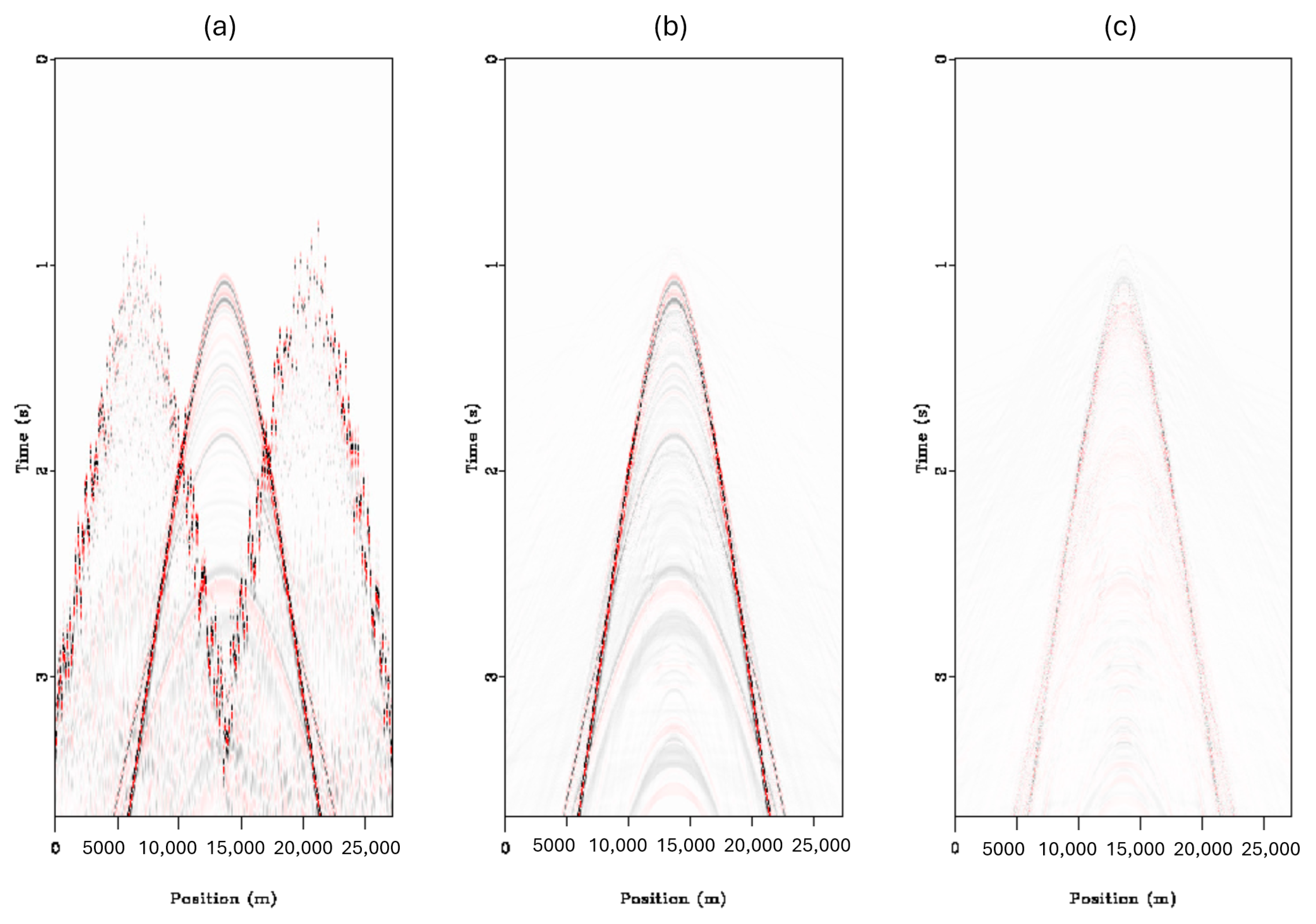
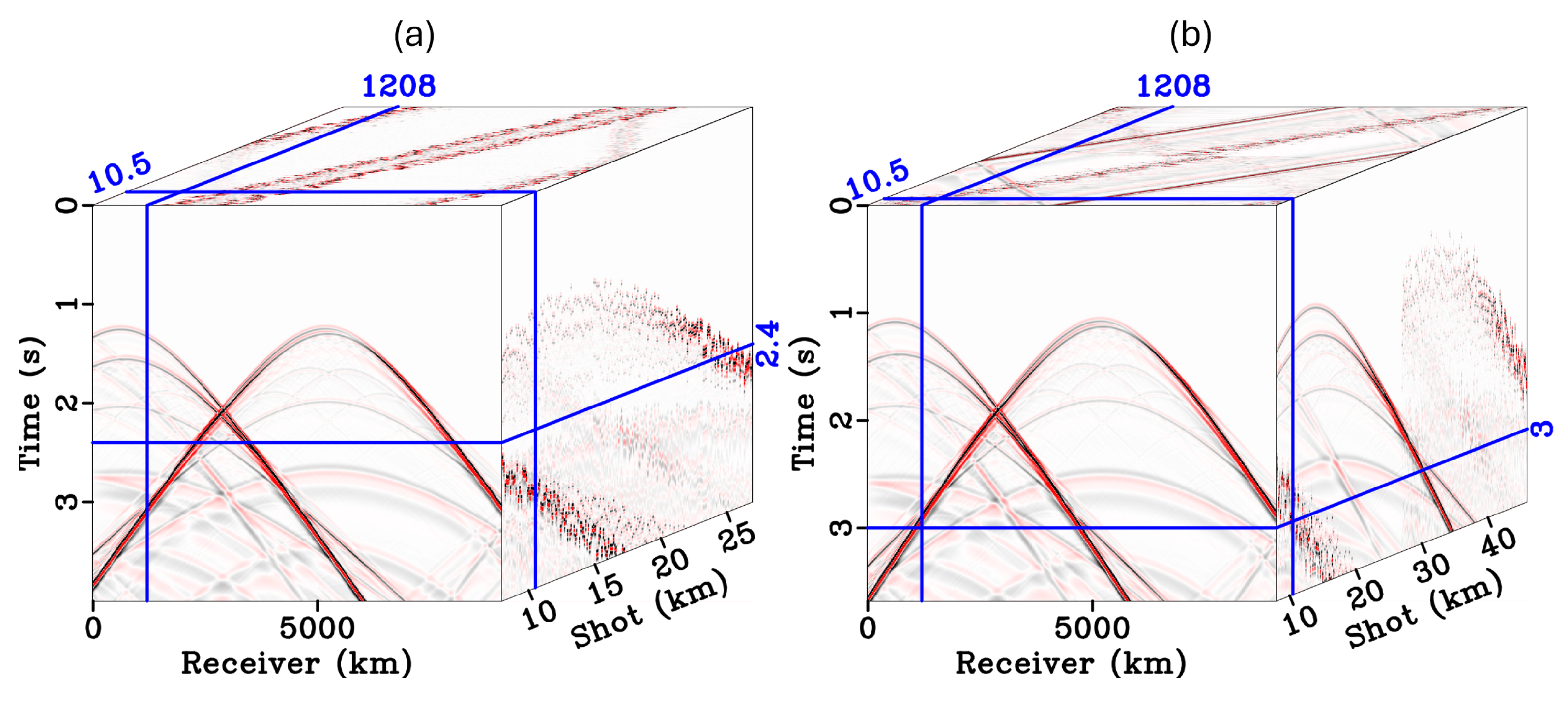
We can also use the sparse inversion to demonstrate the denoising approach to deblending using the Radon transform to denoise individual receiver gathers. The denoising approach first applies pseudo-deblending to the blended data to return a dataset in standard acquisition frames, seen in Figure 1b, which then allows for the separation of the shots through denoising in the other domains. The general denoising process using sparse/robust Radon first applies the adjoint blending operator to the blended data, b:

$$\tilde{\mathbf{D}}=\mathbf{b}{\mathbf{\Gamma }}^H,$$

(10)

Then the pseudo-deblended data are used in the inversion with the following objective function to denoise using the Radon transform:

$$\left|\right|{\mathbf{W}}_{\mathbf{r}}(\tilde{\mathbf{D}}-\mathbf{Rm}){\left|\right|}_p^p+\mu \left|\right|{\mathbf{W}}_{\mathbf{m}}\mathbf{m}{\left|\right|}_q^q,$$

(11)

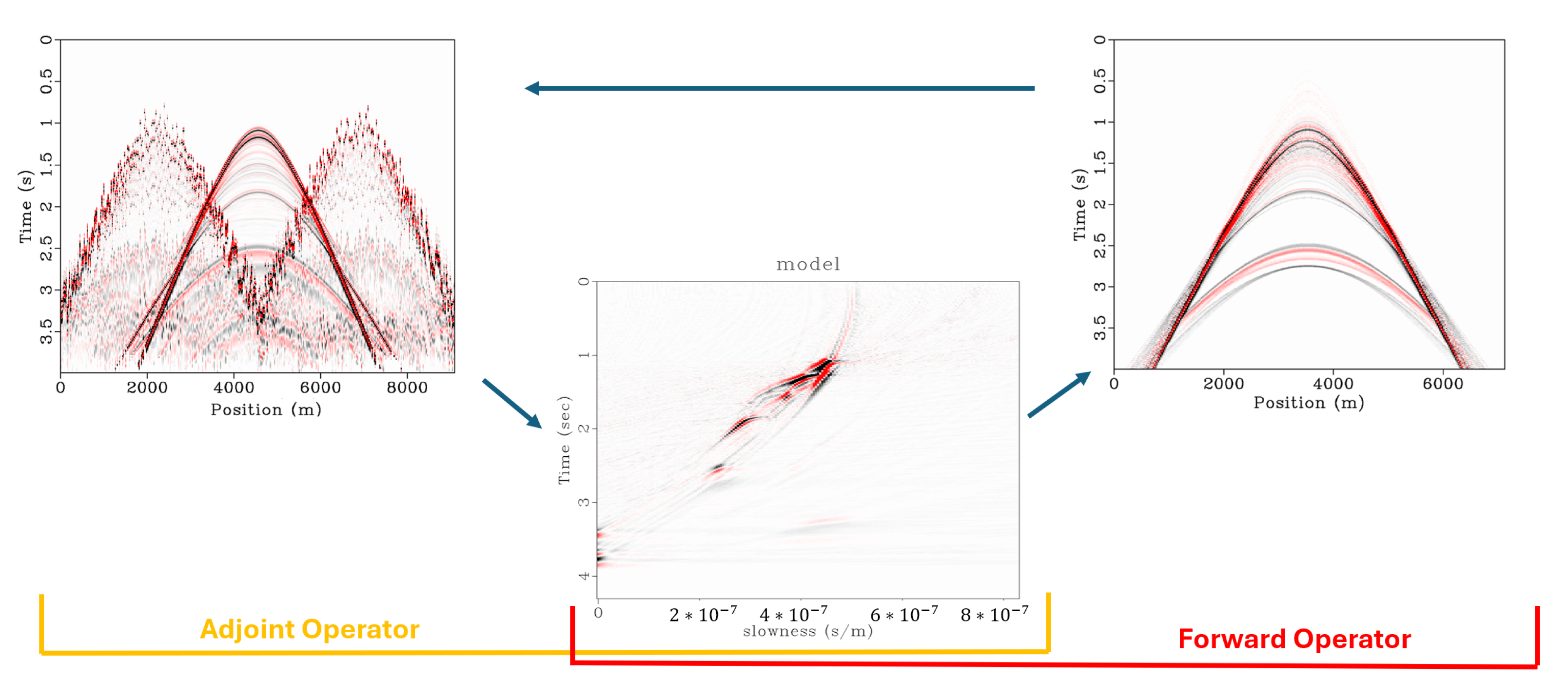
where $\tilde{\mathbf{D}}$ is the pseudo deblended data, $\mathbf{R}$ is the Radon transform operator, $\mathbf{m}$ is the model, $\mu$ is the trade-off parameter, and p and q are the data and model norms, respectively. A graphical representation of Radon denoising can be seen in Figure 2, using standard hyperbolic Radon to downweight spontaneous events in the shot record in an attempt to recover the coherent signal.

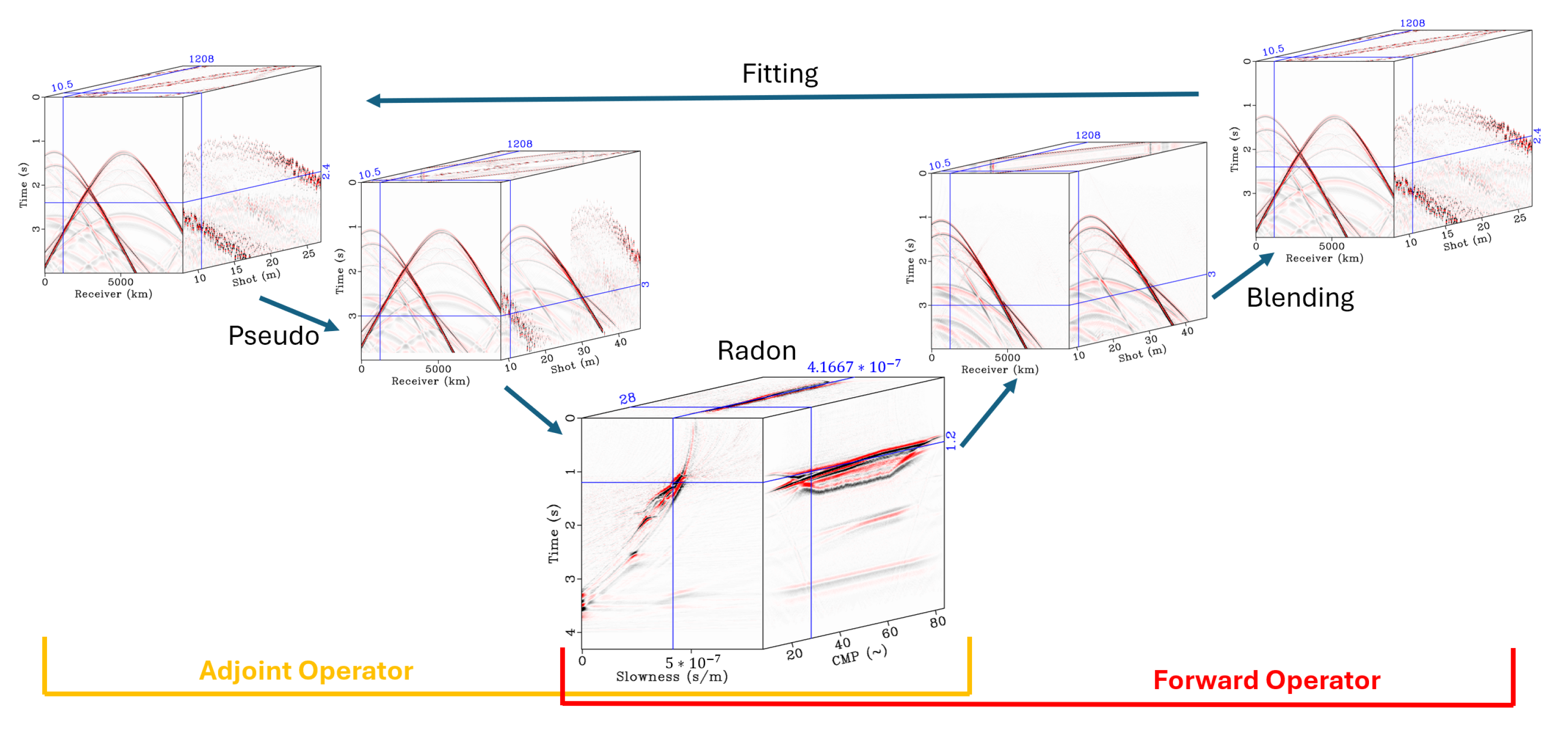
Given that blending noise from one shot record is a signal from another, our sporadic blending noise has the same amplitudes as that of the shot itself. This issue at high blending fold manifests in the high-amplitude noise completely overwhelming sections of low-amplitude events in the signal, which makes traditional filtering-based recovery methods nearly impossible. However, the use of inversion allows us to explain the interfering high-amplitude events and effectively remap only the interfering amplitude, thus allowing us to recover the lower-amplitude signals.The schematic for the inversion-based approach can be seen in Figure 3. However, this approach does not come without its own drawbacks, mainly in the memory requirements, as the entire blending dataset plus the corresponding model must be held in memory. Despite initial expectations, this method does not have any significant runtime difference compared to a similar inversion-based denoising approach, as an inversion must be performed in both cases. When compared to a Radon denoising approach, the inversion approach uses a different objective function as it seeks to incorporate both the blending operator and the Radon operator in the inversion. We can formulate the objective function using the already discussed weights as well as Equation (6):

$$J=\left|\right|{\mathbf{W}}_{\mathbf{r}}{(\mathbf{b}-\mathbf{\Gamma }\mathbf{Lm})\left|\right|}_p^p+\mu \left|\right|{\mathbf{W}}_{\mathbf{m}}\mathbf{m}{\left|\right|}_q^q.$$

(12)

Here, the input is not the pseudo-deblended data, but the blended data, and the operator contains both the blending and Radon operators.

By implementing deblending as an inversion-based operation using the blending and Radon operators together, the system acts like an overcomplete dictionary, where the information is represented and redundant in the pseudo-deblended frames. This aids in convergence as the redundant information explains each other through the remapping of data back to their respective shot frames.

3. High-Performance Computing (HPC) Considerations

The sparse hyperbolic Radon transform is used in our deblending algorithm to reformat the ill-posed blending operator to an inversion problem that uses sparse regularization. This Radon operator allows us to benchmark the performance of a highly parallelizable operation using a series of parallel processing methods. To properly code the HRT to run efficiently in openMP, we send outer offset loops to separate threads to calculate the transform in the adjoint operator; for the forward operator, we then send each outer slowness loop instead. The pseudo-code for the Radon transform can be written as seen in Algorithm 1.

Algorithm 1 Radon Pseudo Code

1:  function  radon 2:       #PRAGMA OMP PARALLEL FOR ▹ insert for parallelization of loop 3:       for q = slowness do 4:             for h = offset do 5:                   $moveout=h^2\ast q$ 6:                   for it = 0 to nt do 7:                         $time=\sqrt{{(it\ast dt)}^2+moveout}$ 8:                         $model[iqNt+it]+=data[ihNt+INT(time/dt\left)\right]$ 9:                   end for 10:            end for 11:      end for 12:  end function

For our implementation in CUDA, we set up a two-dimensional thread configuration with one dimension for each of the time and slowness dimensions in the standard code, then calculated the transform independently for each output cell for each thread. To implement the HRT in openMPI, we send the data pertaining to each shot in the transform to separate nodes and then calculate the transform independently on each node using either the CUDA or openMP methods stated above. We then collect the data at the master at the end of the calculation. The CUDA pseudo-code can be seen in Algorithm 2.

Algorithm 2 CUDA Radon Pseudo Code

1:  __global__ 2:  function CUDA_ radon 3:       int it = blockIdx.x * blockDim.x + threadIdx.x 4:       int iq = blockIdx.y * blockDim.y + threadIdx.y 5:       if (iq >= nq || it >= nt) return 6:       int $iqNt=iq\ast nt$ 7:       double $timemax=dt\ast nt$ 8:       for h = offset do 9:             int $ihNt=ih\ast nt$ 10:           double $moveout=h^2\ast q$ 11:           double $time=\sqrt{{(it\ast dt)}^2+moveout}$ 12:           $model[iqNt+it]+=data[ihNt+(INT\left)\right(time/dt\left)\right]$ 13:     end for 14:  end function

Because a significant number of parallel applications use multidimensional data, the CUDA API groups thread blocks into multiple dimensions, up to three. This is beneficial to the implementation of Radon as there are generally three data dimensions for the transform, one each for offset, time, and velocity. However by assigning each of our variables to a dimension, we can eliminate their respective loops, but this is not the most efficient way to implement the algorithm. Because the model is an accumulation across the offset dimension, we would encounter a data race if the offset dimension h is executed in parallel. If the offset were set as a third thread dimension in CUDA, an atomic operator would be required; this was initially tested and produced significantly slower results than the algorithm provided above. By only parallelizing the two grid dimensions, we avoid the need to use atomic accumulation operators, which can cause significant slowdowns, with each thread performing work for each grid cell in what can be called output-aligned optimization.

This algorithm is interesting in that most of it can be optimized in parallel, but there exist many challenges to proper parallelization. The main challenge of optimizing and parallelizing the algorithm is due to the large memory swaps required for every iteration. These memory issues arise due to the constant need to change domains in the blending operator, resulting in large-scale non-sequential access to the data. The other challenge we face is that this algorithm cannot be properly parallelized across distributed memory systems (servers) using openMPI, as the gradient calculation at every iteration needs to be calculated using the blended operator which requires resorting all data. Since distributed memory in clusters requires splitting the dataset across nodes instead of keeping it all in the master node’s RAM, the resorting process imposes a very difficult challenge for an openMPI implementation. Due to this requirement, each node in a cluster would need to send data back after every calculation to calculate the next step, and then the master will need to resend the results back to each node. For our implementation in CUDA instead of using multiple nodes, we utilize a single high-performance machine, where both the Radon and the least-squares descent algorithm are rewritten using CUDA kernels.

4. Results

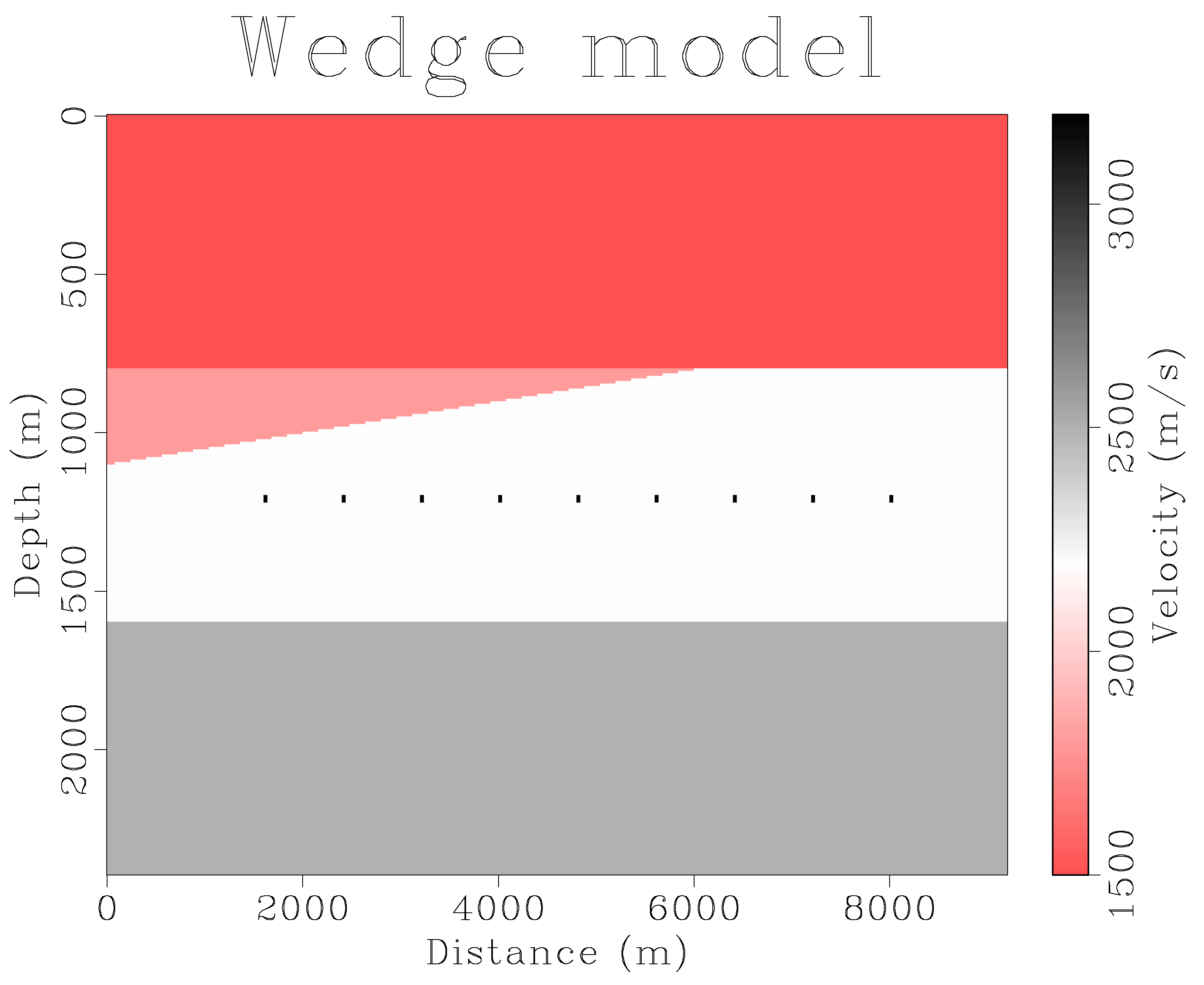
As our test data are mainly synthetic and marine data, we assume that the data space is free of outliers; thus, we utilized the ${\ell }_2$ in the data space, for a mixed norm ${\ell }_2$-${\ell }_1$ inversion. For our testing, we utilized three datasets, two that were created synthetically through finite difference, and one real-world marine dataset from the Gulf of Mexico that was numerically blended. For the synthetic datasets, finite difference modelling was run with 300 shots and 300 receivers evenly spaced at the surface. The first dataset and the most simplistic is the wedge model dataset seen in Figure 4. The wedge model consists of two layers, one triangular wedge, and a set of hard points to test the reconstruction of low-amplitude diffractions. The wedge data were blended with two overlapping shots with delay times randomized between 0 and 400 samples.

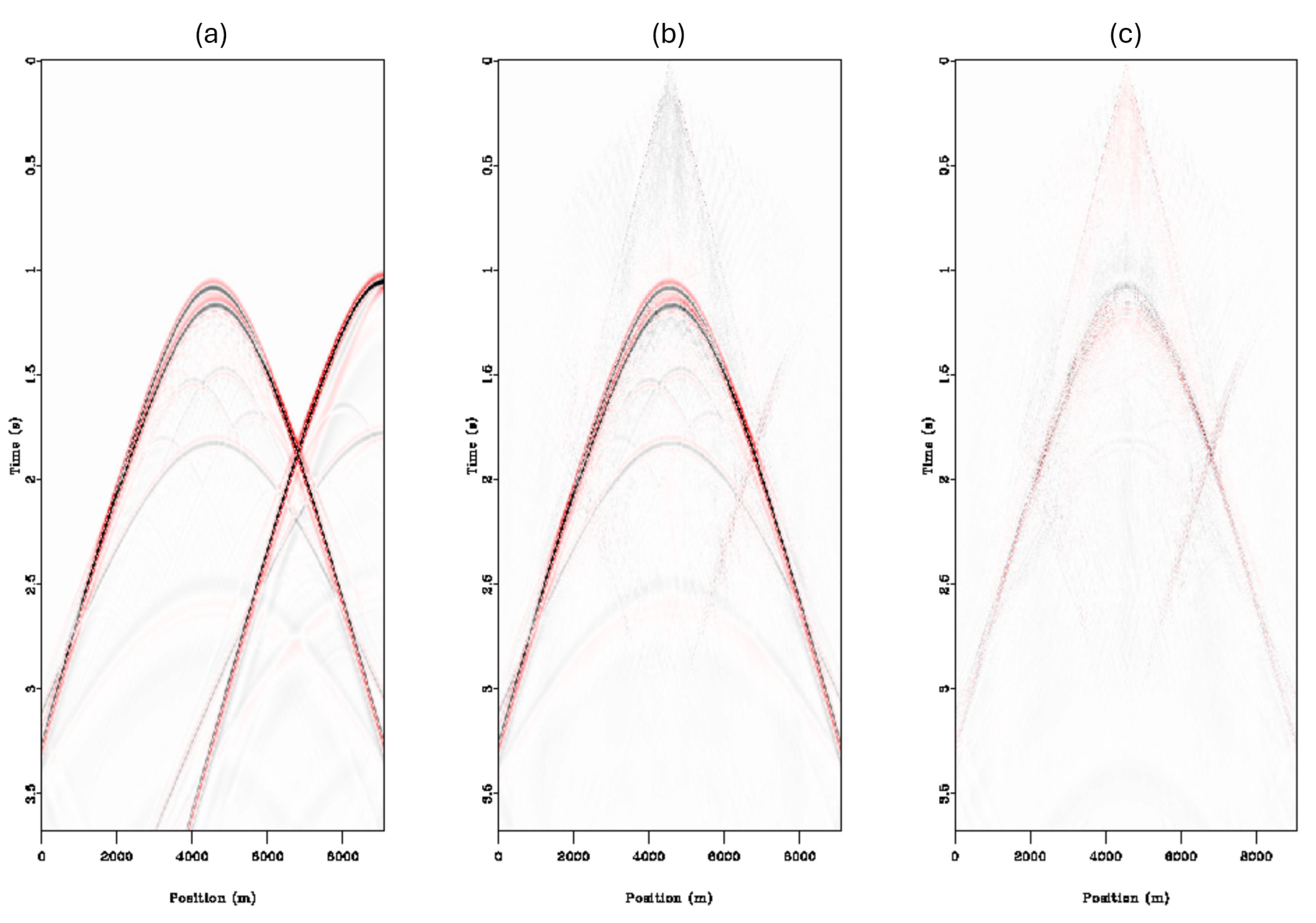
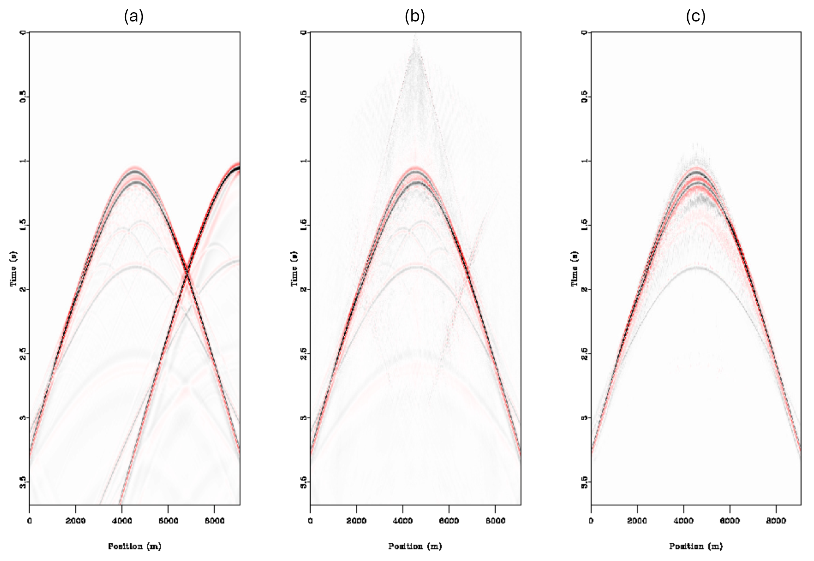
The deblending can be seen in Figure 5, where the blending noise seen in the pseudo deblended data in Figure 5b is removed through inversion in Figure 5c. Subsequently, the results were transformed into the shot domain, as depicted in Figure 6.

Despite some residual interference in the blended shot, the deblending process effectively removed the secondary interfering shot and retained the target shot well, including the diffractions. These can be observed near the top of both Figure 6b,c.

A comparison of our inversion method and a denoising method is shown in Figure 7. The denoising method also utilizes the sparse HRT as a denoising engine to remove the random blending noise in the pseudo-deblended gathers. The primary distinction from the inversion method is that the denoising approach does not involve the blending operator. In the CMP domain, the high amplitudes of the blending noise make direct removal through general noise reduction methods difficult. This is because differentiating noise from data becomes increasingly difficult as the blending noise has the same amplitude as the signal we aim to recover. Without the additional information that the blending operator provides, this similarity makes it challenging to discern which parts of the data are noise and which are coherent signals. As can be seen in Figure 7, the denoising result successfully deblended the data, but at the cost of the lower-amplitude data of the diffraction arrivals, which were removed along with the blending noise.

Synthetic test number 2 was generated via finite difference using the standard Marmousi model [21]. As test 1 showed that our deblending engine effectively deblended our data, we decided to make test number 2 more of a stress test, one in which a non-inversion-based deblending method would have difficulty effectively deblending. We significantly increased the difficulty by reducing the range of our random delay times and also increasing the number of overlapping shots to five up from two, conditions we do not expect to see in the real world currently. 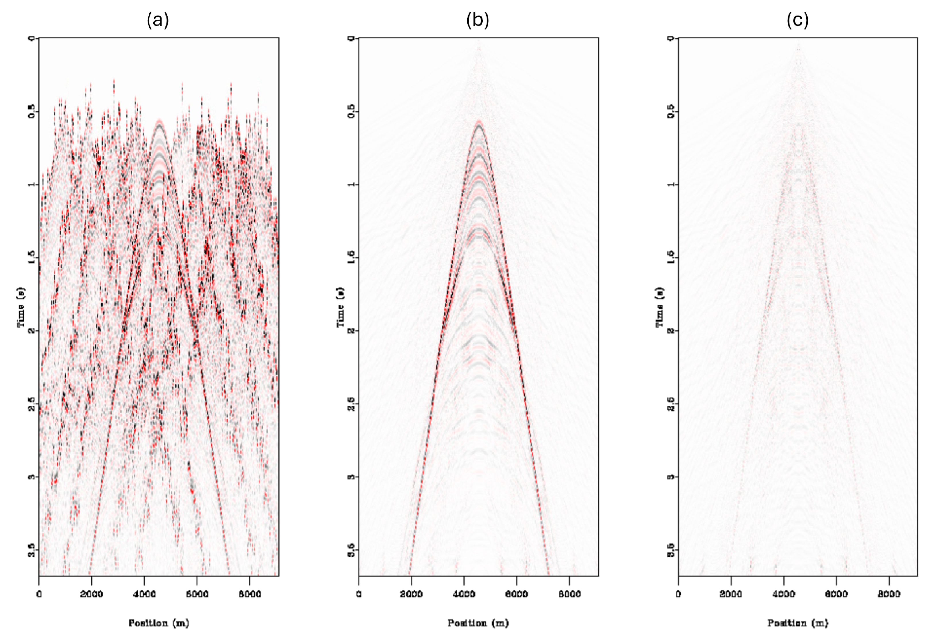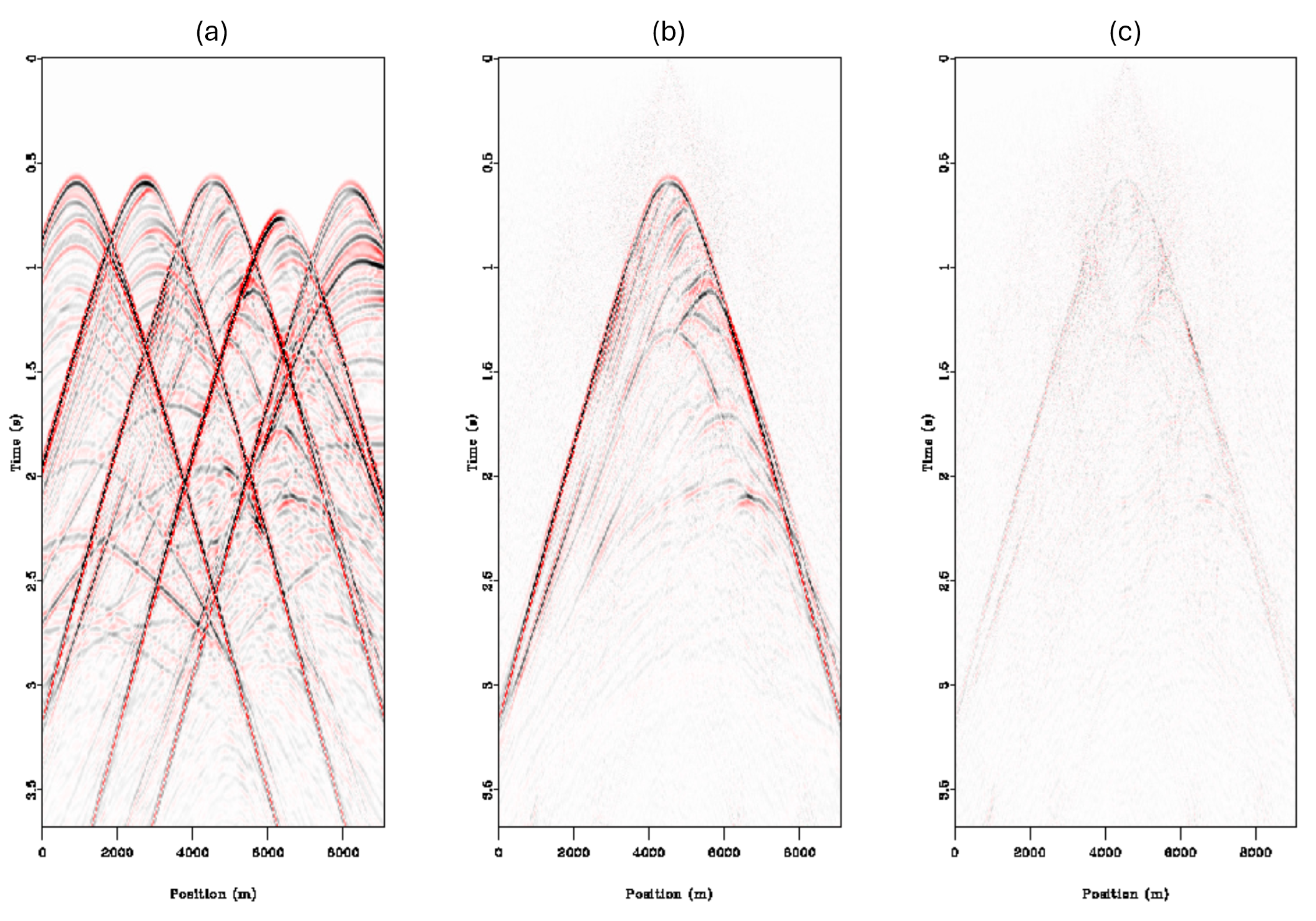Figure 8a shows the blended data in the CMP domain; it is easy to visualize how difficult it would be for a normal denoiser without the blending operator to distinguish the data from the interference in this image.

Analyzing the results of the second test, we can see in Figure 8 that our recovery of low-amplitude reflections is effective even when completely overwhelmed by high-amplitude interference from other shots. Taking a look at the reconstruction error for the shot domain in Figure 9, we can see that the main differences are reduced amplitudes of the higher-amplitude events and the introduction of very low amplitude background noise; we believe that the amplitude error may come from enforcing too much sparsity in the model space, which generally causes these issues in high-resolution Radon, or not fully separating the blending shots and smearing the higher amplitudes across the data as background noise.

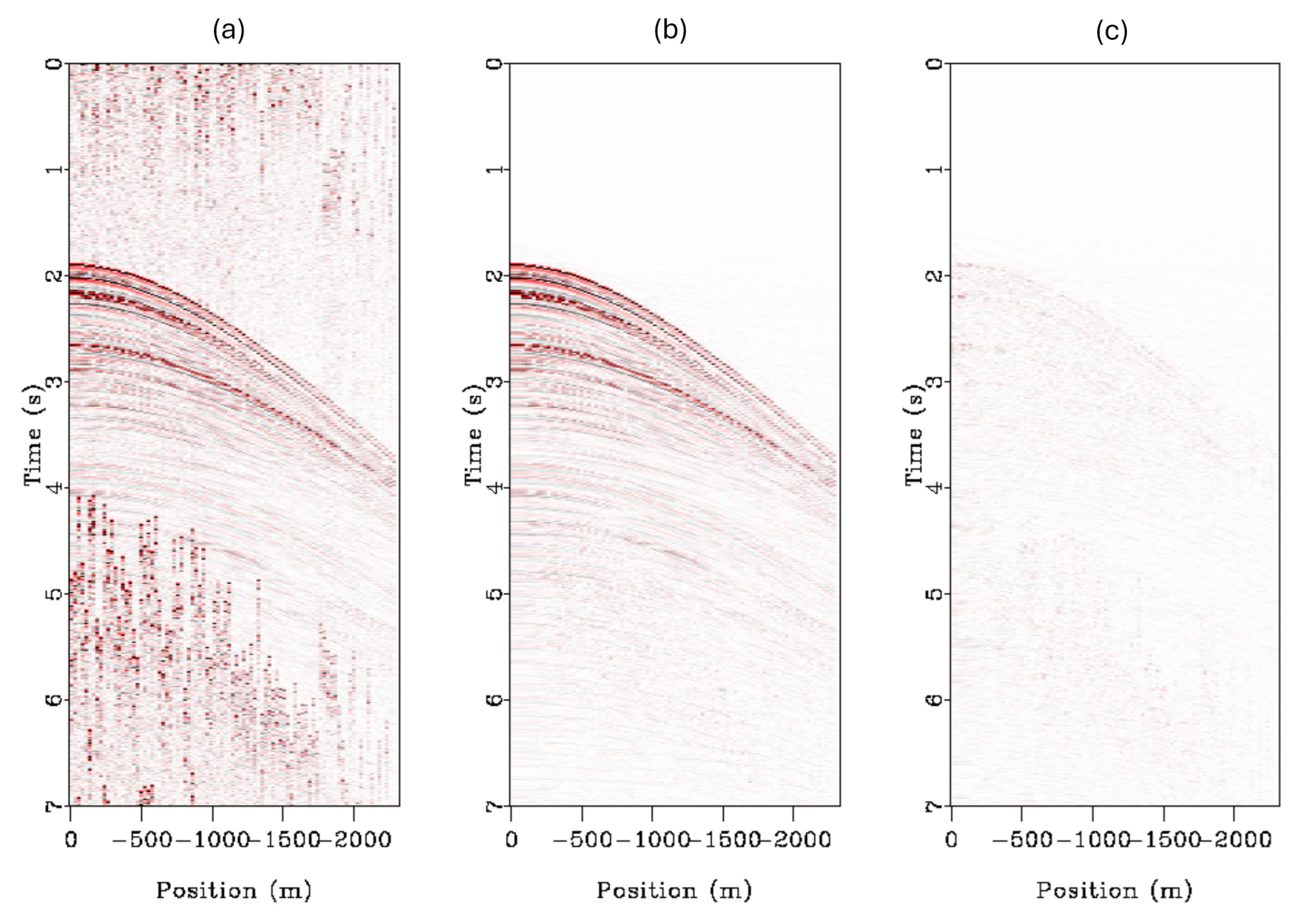
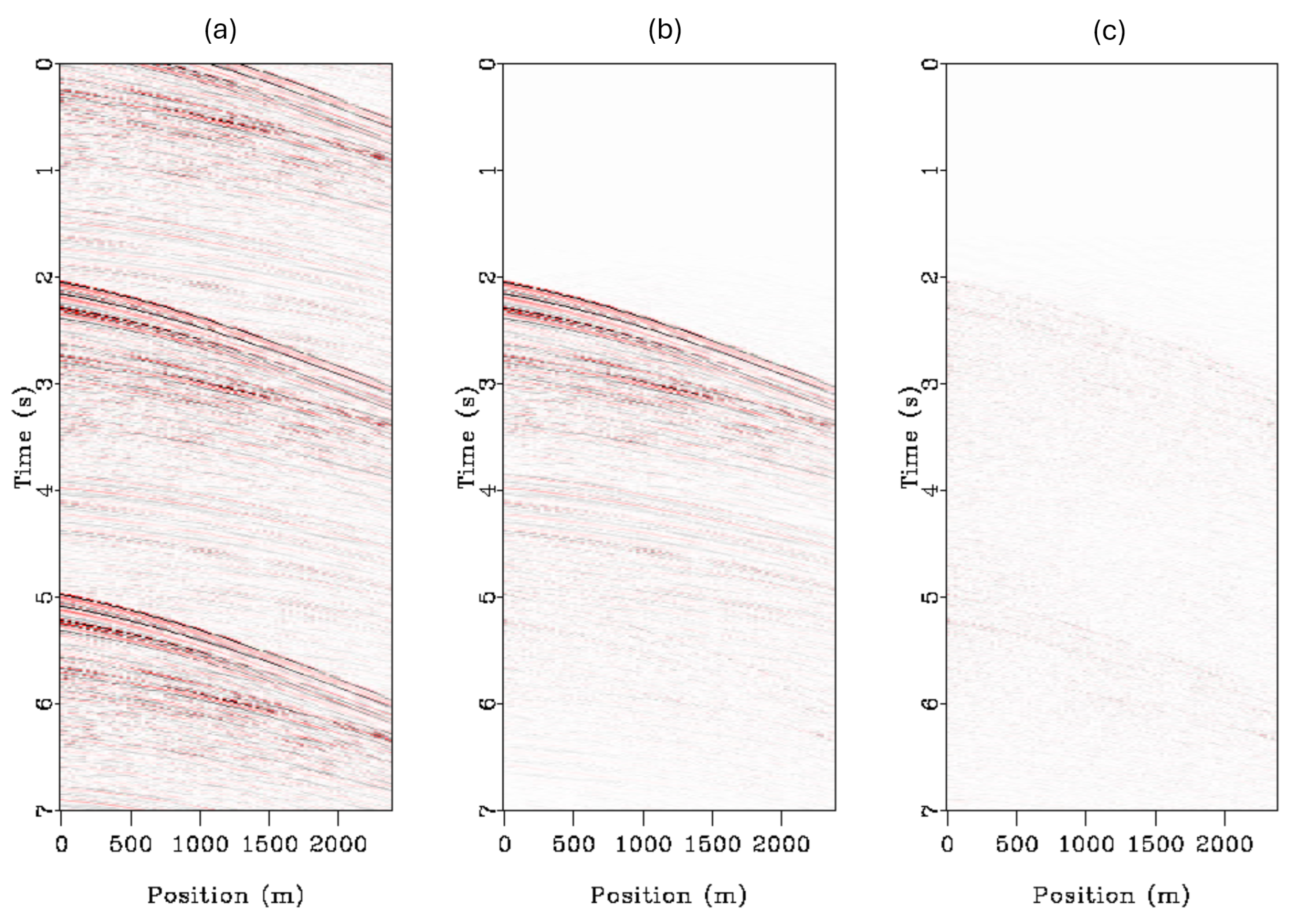
Our final test was a real-world dataset pulled from the Gulf of Mexico, known as the BP Tiber WATS dataset [8,22], which was then numerically blended. The blending scheme was configured differently compared to the others, as this was also a test of another acquisition schedule known as continuous listening. In continuous listening, we effectively have a single supershot, as the data are recorded until all shots are fired and shots are allowed to overlap. The cut-down dataset consisted of 90 shots and 90 receivers, with a shot-to-shot overlap of 70% randomized between 0 and 200 samples. The results of the deblending of the Gulf of Mexico dataset can be seen in the CMP domain in Figure 10 and the shot domain in Figure 11. Analyzing the results, we can see that the deblending algorithm is exceptionally effective at shot separation on the real-world dataset, with good recovery of all events seen in the data. The main error we can observe is that in the shot domain, shots are not perfectly deblended, and some amplitude from the trailing shot can still be seen in the recovered shot. This can be observed around 5.2 s in Figure 11c.

Limitations to this approach lie in the assumptions inherent in the use of the hyperbolic Radon transform. The main assumption of this approach is the hyperbolic trajectory of all seismic arrivals, which are expected to be accurately represented in Radon space. However, this presumption becomes problematic when considering the unique characteristics of land seismic data. The statics inherent to land data can induce vertical shifts in the samples, deviating from their hyperbolic alignment. Such discrepancies lead to an ineffective mapping in the Radon domain and potentially compromise the integrity of the deblending process.

We ran both the deblending algorithm and Radon transform algorithm on a range of different hardware to show the performance of the algorithms using the different parallelization methods in different conditions: a laptop, two workstations, and our in-house server cluster. The laptop utilizes an Intel i7 8750H 6-core CPU with an Nvidia RTX 2060 MAX-Q GPU, the first workstation is equipped with an AMD Threadripper 3960× 24-core CPU, with an Nvidia RTX 3080Ti, and the second workstation has an Intel i7 9800× 8-core CPU equipped with an Nvidia RTX 2060-super GPU. These results can be seen in

Table 1. Table of average runtimes for Radon and least squares deblending on different machines.

Processor (API)	Radon Transform Time (s)	LS Deblending Time (s)
i7 6800k 6-core (openMP)	4462	2590
i5 8600 6-core (openMP)	3773	1748
i7 8750H 6-core (openMP)	4044	2203
i7 9800× 8-core (openMP)	2715	1390
TR 3960× 24-core (openMP)	1123	581
RTX 3060 (CUDA)	147	174
RTX 3080Ti (CUDA)	108	142
RTX 2060 Max-Q (CUDA)	184	206
RTX 2060 Super (CUDA)	157	198
TR 3960× (openMPI)	420	—

. The Runtime between the Radon transform and the deblending algorithm cannot be directly compared as they were performing different tasks; the relative difference in the runtime between different hardware shows the effect the sorting has on the different implementations.

It can be seen that there is a significant computational advantage in moving from CPU processing (openMP) to GPU-based processing (CUDA). The openMPI results show a significant speedup compared to the openMP results and close the gap with the CUDA results; this speedup can mainly be attributed to the coarser-grained nature of the openMPI. The openMPI implementation shares fewer resources between threads; thus, less overall memory management has to be performed by the system, at the cost of overall RAM space as more copies of data are made. In standard Radon transform testing, the CUDA-based code reduced compute time by over an order of magnitude compared to the openMP version; after the introduction of the least-squares algorithm, the advantage diminished by a large amount. Due to the openMPI distributing all work, including the LS optimization across the nodes, it can run the LS optimization in a parallel fashion that neither the openMP nor CUDA code can, resulting in an overall faster computational time versus openMP and approaches to the CUDA implementation. OpenMPI deblending, however, cannot be properly implemented as the host node must collect all data from the other nodes to perform the LS calculation every iteration; this results in large memory transfers across the network which incur a significant latency and transfer rate hit. The overhead associated with the openMPI implementation is so large that we did not notice a benefit in our prototyping of the program as compared to even single-threaded runtimes. It must be noted, however, that openMPI used the largest amount of RAM in this exercise, about 122 GB, compared to the openMP and CUDA implementations which used 8 GB of RAM and 8 GB + 8 GB (mirrored) VRAM, respectively. The main trade-off between a CUDA/GPU-based approach and an OpenMP approach would be that of speed versus portability; the CUDA approach is significantly faster but requires an Nvidia GPU, while the OpenMP approach will work on any device that supports OpenMP parallelization in the compiler, which is any modern CPU that exists on the market.

5. Conclusions

We proposed a method for deblending that employs a linear inversion of a composite transform operator in the CMP domain. This inversion, when used with the blending operator, allows us to predict and remap, rather than eliminate, interfering shot information. This, in turn, facilitates the accurate recovery of low-amplitude events, even in data that are heavily blended. The implementation of a sparse constraint on the inversion algorithm enables us to arrive at a unique solution that enhances the coherency of the signal in hyperbolic arrivals. Furthermore, the use of hyperbolic Radon transforms in the CMP domain provides us with an operator that is efficient and well matched to our data, promoting coherence in our recovery and circumventing aliasing issues. Consequently, we are confident that our inversion approach is an effective strategy for deblending simultaneously sourced data while safeguarding low-amplitude events. We have also explored additional methods to accelerate this framework through applications on both the CPU and GPU, each with its own set of advantages and disadvantages.