Article

Particle Swarm Optimization-Based Model Abstraction and Explanation Generation for a Recurrent Neural Network

1
Institute of Logistics Science and Engineering, Shanghai Maritime University, Shanghai 200120, China
2
School of Accounting, Nanjing University of Finance and Economics, Nanjing 210023, China
*
Authors to whom correspondence should be addressed.
Algorithms 2024, 17(5), 210; https://doi.org/10.3390/a17050210
Submission received: 18 April 2024 / Revised: 10 May 2024 / Accepted: 10 May 2024 / Published: 13 May 2024
(This article belongs to the Special Issue Deep Learning for Anomaly Detection)

Abstract

:
In text classifier models, the complexity of recurrent neural networks (RNNs) is very high because of the vast state space and uncertainty of transitions, which makes the RNN classifier’s explainability insufficient. It is almost impossible to explain the large-scale RNN directly. A feasible method is to generalize the rules undermining it, that is, model abstraction. To deal with the low efficiency and excessive information loss in existing model abstraction for RNNs, this work proposes a PSO (Particle Swarm Optimization)-based model abstraction and explanation generation method for RNNs. Firstly, the k-means clustering is applied to preliminarily partition the RNN decision process state. Secondly, a frequency prefix tree is constructed based on the traces, and a PSO algorithm is designed to implement state merging to address the problem of vast state space. Then, a PFA (probabilistic finite automata) is constructed to explain the RNN structure with preserving the origin RNN information as much as possible. Finally, the quantitative keywords are labeled as an explanation for classification results, which are automatically generated with the abstract model PFA. We demonstrate the feasibility and effectiveness of the proposed method in some cases.

Graphical Abstract

1. Introduction

Deep learning is a branch of machine learning in artificial intelligence (AI) that uses artificial neural network architecture to learn from data and mimic human thinking patterns [1]. A recurrent neural network (RNN) is a typical deep learning model that takes in sequence data. It connects all units in a chain-like manner and processes them along a time-ordered or logic-ordered sequence [2]. The RNN has been broadly applied in natural language processing (NLP) fields, such as text classification, sentiment analysis, machine translation, and other time series analysis areas. For the text classification in NLP, one of the security threats in RNNs, i.e., adversarial text attacks, is increasingly attracting people’s attention. Real-world application scenarios for adversarial text attacks include spam detection, harmful text detection, and malware checking [3,4,5]. More and more text classification systems are deploying RNNs with enormous layers and neurons, and security is significant for these systems. One of the troubles is that RNNs will produce results out of the attacker’s unfriendly purpose with ulteriorly attacking, which may lead to a catastrophe [6]. The users or developers need to know what kind of abnormal behavior of RNNs is involved in the system, that is, providing clear explanations for the output results. With appropriate explanations, the classification results can be more acceptable, and the undesirable RNN model can be repaired under some guidance [6,7]. Explainability is an important dimension for developing trustworthy RNNs, and it is also the guarantee for the large-scale application of RNNs.
Like other deep learning models, it is almost impossible to fully understand the internal structural organizations of a large-scale RNN and clarify the communication paths between its neurons [8]. When an RNN model contains vast layers, it is difficult to adopt a suitable mechanism to describe the decision-making process in the RNN. Even if we can list all the weights, inputs, and outputs of activation functions for each neuron node, we still do not know how those large and constantly changing numbers are organically combined to complete a prediction or decision-making task. Therefore, users either have little knowledge of what the system makes decisions based on or cannot afford the time and space costs to handle the dynamic changes and every static detailed parameter of RNN neurons. Providing explanations for RNN text classification results is an important and valuable research topic.
In recent years, some works have attempted to achieve the explainability of RNN models through model abstraction techniques [9,10]. Model abstraction can obtain a concise approximate model for an original RNN, which removes irrelevant or trivial information and keeps specific properties under consideration. Explaining RNNs on an abstraction model is beneficial. Firstly, the state space of the abstraction model is significantly reduced, which can effectively save time and space to visit the original RNN, especially when the dataset is large [11]. Secondly, some practical model analysis and verification techniques can be applied to the abstraction model to explain the original RNN [12]. This undoubtedly meets the inherent requirement of transparency in explainability principles. Thirdly, it is difficult and costly to reverse engineer an abstraction model to reproduce an RNN model, which provides reliable protection for the original RNN [13].
The main challenges in applying model abstraction to explain RNNs are as follows. Firstly, it is not easy to map the specific insertion patterns with neural activation, unlike convolutional neural networks (CNNs), which have a fixed number of neurons and play a particular role in feature extraction. The network layers in RNNs typically cannot maintain the same potential spatial functions due to their dynamic behavior over time, and the length of different input sequences varies with the dynamic behavior over time. Secondly, the text data processed by the RNN is essentially discrete, which makes it more difficult to abstract than pixels in image data.

1.1. Related Works

RNN model abstraction has accumulated some works. According to the method of model abstraction, they can be divided into two categories: active learning abstraction and passive learning abstraction. Passive learning refers to constructing abstract models based on one or a series of traces of RNNs [14]. Active learning involves conducting experiments or tests to complete the abstraction model by the learner adaptively. The basic idea for active learning is based on the MAT (minimally equal teacher) framework proposed by Dana Anglin [15]. Until now, most effective active learning algorithms conform to the MAT framework [16]. According to the abstract model type, they can be divided into a decision tree, non-deterministic and deterministic finite state automaton (NFA/DFA), discrete-time Markov chain (DTMC), weighted finite automaton (WFA), probabilistic finite automaton (PFA), etc. According to the purpose, i.e., the subsequent work, of model abstraction, they can be separated into two branches: abstract RNNs for explaining and abstract RNNs for verifying or analyzing. We will review the existing related works of RNN model abstraction according to the subsequent purpose.

1.1.1. Explanation of RNNs Based on Model Abstraction

Hou et al. [17] propose a learning finite state automata (FSA) method to explain the impact of gate units on the gated RNN mechanism. This method empirically explores the text sentiment analysis tasks of multiple gated RNNs. The abstraction model FSA visually explains the RNN decision-making process, which explains the semantic aggregation state in RNNs. However, the article does not provide a global quantitative explanation from the perspective of feature influence, and the learned FSA cannot express the characteristics of probability transition between states. Fan et al. [18] use an evolutionary merging algorithm to learn a simple non-deterministic model NFA. This abstraction process loses too much information, as the expression of NFA is limited, which leads to the accuracy being very low. Wei et al. [19] propose a WFA model learning technique for RNNs and provide ask-oriented global explanations at the word level, guided by transformation matrix embedding. It has better accuracy and scalability than the L* algorithm.

1.1.2. Formal Verification or Analysis of RNNs Based on Model Abstraction

Yellin and Weiss [20] learn the deterministic finite automata (DFA) from sequences of RNNs using the algorithm in [21] and use the pattern rule sets to infer context-free grammars (CFGs). Context-free language (CFL) rules are more suitable for natural language processing than automata. This algorithm is relatively easy to understand and can extend to non-context-free languages. However, the extracted DFA often contains some noise, which either comes from RNN training or the inherent noise factors of the L* algorithm. Therefore, interference patterns are usually inserted into DFA, causing the results to deviate from the pattern rule set. Barbot et al. [22] propose an active learning algorithm for extracting visible pushdown syntax for RNNs. It learns DFA and then uses A* search to extract the CFGs, which are applied to a surrogate model trained in context-free language. The limitation of this article is that it mainly targets visual pushdown languages, namely, structured data (annotated language data, programs, XML documents, etc.), and its practical applicability is limited. Hong et al. [11] propose an AdaAX method instead of identifying patterns on pre-determined clusters, which identifies a set of finer-grained patterns in direct data. Then, these small sets gradually merge to form states, allowing users to trade fidelity for lower complexity adaptively. This method ultimately learns the DFA model and mainly focuses on model rule extraction. It has some shortcomings, such as low automation and high computational costs. Wang et al. [23] learn the RNN as a DTMC, in which state traces extraction part uses the predicate abstraction technique. Afterward, genetic algorithms were used for state merging. Weiss et al. [24] learn PFA from the RNN by adjusting the L* algorithm and use PFA for formal validation of RNN language models. Dong et al. [25] use unsupervised learning algorithms to obtain discrete partitions of RNN state vectors, construct symbol traces, and apply the AAlergia algorithm [26] to learn PFA. This method has robust scalability, and it has been applied to adversarial sample detection in large-scale text classification tasks. However, the learning accuracy of this algorithm is slightly inferior, as a single AAlergia algorithm is used in the state merging process. Its interval contraction speed is slow, as it adopts the interval optimization strategy of golden section search in model selection, so there is still space for improvement.

1.2. Contributions

This work focuses on model abstraction and explanation generation of RNNs for text classification. As shown in Section 1.2, there are two main shortcomings of current model abstraction for RNNs: difficulty in dealing with large-scale RNNs and excessive information loss in abstract models. To deal with these, this work proposes two optimizations: using the PSO (Particle Swarm Optimization) algorithm to optimize the process of generating abstract models for RNNs, which can cope with large-scale RNN models and improve the scalability of abstract methods, and using PFA as an abstract model for RNNs, which can address too much information loss during the abstraction process and improve the accuracy of abstraction model. In a word, this work proposes a model abstraction and explanation generation framework for RNNs based on the PSO algorithm. The contributions of this work are as follows:
  • Constructing abstract state traces with k-means clustering and building a tree structure;
  • Designing a PSO algorithm to search and learn the abstraction model PFA and find PFA with better complexity and similarity performance when the level of abstraction is constant;
  • Using the abstract model PFA to automatically generate an explanation of the importance of input features in classification tasks;
  • Exploring the practicality of our framework to adversarial text detection in RNN text classification.

1.3. Structure of This Paper

In Section 2, there is an introduction to basic knowledge, including an overview of RNNs and a formal description of PFA. We present, in detail, how to generate clustering traces, how to use PSO to learn PFA, and how to generate RNN explanations based on PFA in Section 3. In Section 4, we evaluate and compare the framework’s performance through some cases. Section 5 analyzes the effectiveness and usefulness of the framework. We conclude and point out the future work in Section 6.

2. Preliminary

2.1. RNNs

Recurrent neural networks bring memory units that are different from other traditional neural networks. The characteristic of the RNN structure is that it has a certain number of serial-connected subnetworks. Its hidden nodes can also store specific historical information, as this memory function is similar to the human brain, allowing RNNs to process recognition tasks like the human brain. It focuses more on helpful information so that it can skip irrelevant messages in the dataset. Its basic unit structure is shown in Figure 1.
In the text classification task, the input is the word vector of the text input word at time step t = i, and the hidden layer output is h i = f u x i + w h i 1 where f ( ) represents the activation function. It can be seen here that the input of the hidden layer at the current step includes the output of the hidden layer from the previous steps, which reflects the meaning of “recurrent” and is also one of the underlying reasons for the memory mechanism in RNNs. The output is o i = s o f t m a x v h i , in which s o f t m a x is the activation function of the output layer. In the above formula, u, v, and w are weight matrices of input, hidden layer, and output vectors, respectively.
The state diagram conforms to a mathematical model of human cognitive patterns and habits. Although state diagrams are widely used in the field of computational science, their universal applicability has also inspired researchers in modern machine learning. The academic community recognizes that since the RNN is complex, we can transform it into a state diagram model and indirectly study the RNN using well-established methods of state diagrams. As a result, many researchers have made crucial contributions, attempting to simplify deep neural networks using state diagram models. Many of these studies have indeed made commendable progress, including L* and various improved methods based on L*. Next, we will introduce one of the state diagram models, namely, probabilistic finite automata.

2.2. PFA

In the automata theory, an automaton does not refer to a concrete machine but rather a dynamic mathematical model of discrete systems that can transform and process information [27,28]. Probabilistic finite automata (PFA) is a branch of automata that is a structured representation of discrete mathematical models. The theory of automata studies the mathematical theory of analyzing and synthesizing automata, an essential branch of control theory. Compared with non-probabilistic finite automata, the characteristic of probabilistic finite automata is that its state transition process provides probability values, which can quantitatively express the randomness of the state transition process [29].
The research fields of automata theory are divided into three categories: abstract theory, structural theory, and self-organization theory. In abstract theoretical research on automata, the structure of the automata itself and the specific forms of its input and output signals are not considered, and the automata is treated as a mathematical system to study its general mathematical properties. The study of the structural theory of automata is a further development of the abstract theory of automata. Structural theory research focuses on the synthesis of automata, methods for constructing automata from meta-automata, and techniques for encoding meta-signals transmitted through input and output channels. The self-organization theory of automata is the result of the development of abstract theory and structural theory of automata. Self-organization theory involves many aspects, such as neural networks, pattern recognition, and other artificial intelligence. In 1969, King-sun Fu et al. applied the concept of fuzzy neurons to automata theory, leading to new developments in the research of neural network theory and the application of automata theory to study the behavior of complex systems, such as RNNs [18,25,30,31]. Below is the mathematical definition of PFA.
Definition 1.
PFA is a tuple of five elements, defined as the alphabet < Σ , Q , δ , Q 0 , Q f > , where Q refers to the possible finite states of the initial, intermediate, and final states observed by the RNN. δ :   Q × Σ Q is the labeled transition function. The transition probability of each edge in the automaton is recorded in δ . Q 0 and Q f are the finite starting state set and the accepting state set, respectively. Below, we will use a simplified statement to classify positive and negative labels as an example.
Example 1.
Case of Converting the sentiment classification process of “This movie is so beautiful!” in an RNN to PFA.
Assume that the PFA shown in Figure 2 is the state transition process of the sentiment classification involved in this input. Firstly, vectorize the input texts and convert them into PFA input vectors. We set all the words input into PFA as follows: “This”, and its corresponding state name is vectorized to w v 0 , “film” to w v 1 , “is” to w v 2 , “nice” to w v 3 , and “not” to w v 4 . Then, the current string is turned into the vector sequence w v 0 w v 1 w v 2 w v 3 . If the start word of the string w v 0 was read by an RNN, the state of the RNN will transit to state 3, with a transition probability of p 0   =   0.9 . Next, there is a corresponding transition of w v 1 , so its transition probability to itself is p 2   =   0.3 . Then, read w v 2 , and transition to state 2 with p 2 = 0.3. Finally, read w v 3 ; the RNN transitions to an acceptable state 4 with a probability of p 4   =   0.7 . PFA in such a case is represented as the following:
  • Alphabet: The numerical value at the right of the separator symbol “/” on the arrowed line between each pair of states in the graph is a set: w v 0 , w v 1 , w v 2 , w v 3 , w v 4 ;
  • State set: Q = { s 1 , s 2 , s 3 , s 4 , s 5 } ;
  • Acceptance set: Q f is the set { s 4 , s 5 } in the graph, in which the set of acceptance state labels is {P, N}. They are nodes with double-edged circles.
  • Transition probability: A numerical value δ is at the left side of the separator “/” between states of the PFA, and δ represents the corresponding probability of transition between states.
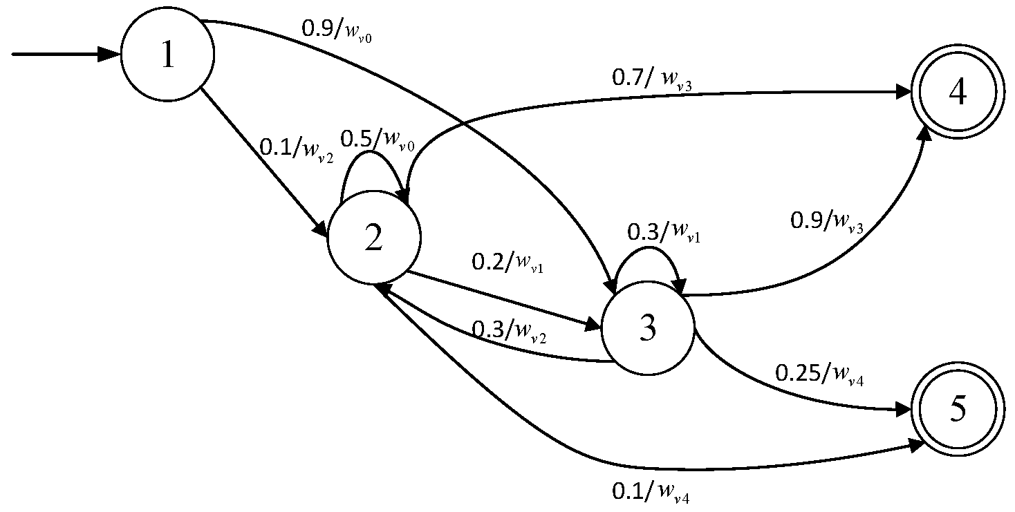
Figure 2. PFA example.
Algorithms 17 00210 g002

3. Model Abstracting and Explaining Framework

This section proposes a PSO-based RNN model abstraction and explanation-generating (called PSO4RNN) framework, as shown in Figure 3. It consists of two main parts: abstraction model learning and explanation generating (called Stage I and Stage II in this Section). Among them, the learning process of an abstraction model mainly includes two steps: state trace abstraction and frequency prefix tree merging (from Step (1) to Step (3) of Stage I). The explanation-generating part (called Stage II below) works based on the learned PFA to explain the classification results.

3.1. Learning Abstraction Model for RNNs

3.1.1. Obtaining the Abstract Traces

The first step in learning a PFA for RNNs is to extract the hidden states. They play a significant role in revealing the internal causal relationships of RNNs, which include hidden layer weight vectors and output layer weight vectors. In addition to the hidden state of an RNN, they also involve processing the state of the input layer, representing discrete texts as numerical vectors. In the field of NLP, the word embedding technique is feasible and effective for word representation. It converts natural language words into digital form, so we can measure their quantitative properties.
If researchers directly obtain all states from RNNs to construct PFA, the construction process will be very cumbersome due to the large observation state table. Therefore, this abstracting technique needs to reduce the number of hidden states continuously. According to the research on RNN model abstraction learning [32,33,34], hidden states with similar behaviors have very close positions in their state vector space, so states with similar behaviors can be integrated into the same region. In Step (1) of Stage I, we use k-means to integrate RNN states, which divide many state vectors into a finite number of clusters to reduce the number of operational state objects in subsequent abstraction learning algorithms. The position vector of the space partition center represents the characteristics of the abstract state. The clustering technique is based on explainable k-means, so abstract techniques ensure explainability in the clustering process. In addition, clustering divides a large number of complex hidden states into a finite number of partitions. This is in line with the natural cognitive pattern of humans in the process of text classification, which is to classify text words based on their meanings and context, judge the importance of numerous words critical to classification results, and then decide the overall class of the whole text.
In the process of abstract states partitioning, appropriate preprocessing (such as word embedding) can reduce the number of input words, the dimensionality of clustering operation input vectors, and the cost of k-means processing. We use a word2vec pre-trained model for word embedding. After the state clustering in the original RNN, it is necessary to construct various abstract state traces. Due to the interweaving of nodes during state partitioning, state transitions also change dynamically. The transitions between different states should be independently recorded and processed. Subsequently, each state transition will be added between the corresponding states, creating a complete sequence from the start to the end state. This yields a state trace. Repeat these steps until all state and model behavior samples create corresponding traces. This process corresponds to Step (2) and Step (3) of Stage I, as depicted in Figure 3.
After sorting out the state traces, the traces will be organized one by one into a frequency prefix tree (FPT). From a practical perspective, an FPT can be considered a special type of PFA, which is a very detailed probabilistic finite automaton. It contains detailed information beyond the user’s needs, often overwhelming the messages that humans should mainly focus on. Therefore, it is necessary to trim the FPT further and reduce the number of useless nodes and edges. Such a process is called learning PFA from the FPT. The following example illustrates a brief process of text classification that abstracts traces and organizes them into a frequency prefix tree. This process corresponds to step (4) of Stage I, as depicted in Figure 3.
Example 2.
An example of trace abstraction for an RNN-based sentiment analysis of movie reviews.
We use PFA in the sentiment analysis case in Example 1 as a description. Firstly, the learned PFA requires segments from comments and then word embedding. If one of the input sentences is s e n 0 , then “This film is nice, I feel satisfied”. Suppose there are 100 sentences in the corpus D c 0 . After word embedding, the words in D c 0 are represented as numerical vectors. The RNN object model is obtained through classical training processes. In s e n 1 , the hidden layer states of words “nice” and “satisfied” are H s 11 , H s 12 , and we record all such results in the corpus as HS = < ( h s 1 , 1 , h s 1 , 2 ) , ( h s 2 , 1 , h s 2 , 2 ) , , ( h s 100 , 1 , h s 100 , 2 ) > . Then, these states of RNN layers are classified into some state partitions.
The formed abstract state trace of the RNN classification process is shown in Figure 4. Assuming these hidden states are s 0 s e n 0 , s 1 s e n 0 , s 2 s e n 0 , they will be organized into a sequence A T 0 . It can be understood as an RNN processing of s e n 0 . All processing paths of sentences in the corpus can be constructed as several traces. In the subsequent process, they will be merged into a frequency prefix tree.

3.1.2. Learning PFA

This whole PSO searching process corresponds to Step (5)–Step (9) in Stage I. This work designs a PSO algorithm for optimizing the search of PFA, with generalization as the objective fitness function. The generalization value can be seen as a quantitative property combined with similarity and complexity. The PSO algorithm merges the frequency prefix tree into PFA, which is obtained from the initial combination of abstract traces. It achieves automatic search during the merging process and makes the merged PFA better fit the behavior of the original RNN.
We set the particle vector of PSO as the position of the i-th particle in space, which is represented as P t x i = P t x i 1 , P t x i 2 , , P t x i D . Unlike the classical PSO algorithm, the solution of the PFA state merging problem is partially presented as a discrete variable, such as the alphabet, so part of the components in the particle space is discrete. For these discrete parts, we adopt measures of partial discrete subsequent decoding for processing. This not only preserves the continuity processing of probability information but also makes reasonable adaptations to the discrete parts. Due to the particularity of PFA learning, we fine tune the traditional PSO based on preliminary theoretical simulation and experimental comparison. In the following, this variant will be referred to as the Partial Discrete Particle Swarm Optimization Algorithm (PD-PSO). We convert the numerical values of certain discrete variables corresponding to particles into integers within the interval [0, N D d ], where N D d is treated as continuous variables to determine the number of possible values for the discrete value of dimension d. In addition, PD-PSO will discretize continuous variables after the algorithm is completed, just like digitizing analog quantities in the field of digital circuits, which may result in quantization errors. The PD-PSO algorithm does not discretize the continuous parts in the searching process.
A good PFA must have two main properties, namely, the similarity between PFA and its corresponding original RNN and the low complexity of PFA itself. Quantifying complexity is relatively easy, but another critical issue is how to determine similarity. Traditional L*-style methods use comparative testing or heuristic algorithms, such as genetic algorithms, to replace comparative testing.
The primary role of PSO is in the merging stage of PFA. The core issue is how to choose a fitness function. The frequency prefix tree obtained from k-means will be transformed into a particle. The target fitness function fit (Ptx) will perform as a guide to optimize the parameters approaching the best fitness and thus obtain the corresponding PFA. The main issue in is controlling the degree of message generalization. The generalization of abstraction models can be seen as a combination of similarity and complexity. The good generalization enables PFA to retain as much essential information about the original RNN as possible, and it is simple enough. Due to the inevitable tradeoffs between these two requirements, it is a long-standing issue that has been discussed in academia. This is also the main reason for the improvement proposed in this work. According to the Bayesian Information Criterion (BIC), a fitness function is constructed based on complexity and similarity, and the optimization objective is defined as minimizing the BIC of the abstract model. Unlike the BIC used in traditional merging algorithms, exporting parameters in PSO4RNN is not based on a golden section search but on a heuristic search. A golden section search is only suitable for the assumption of unimodal functions, but the actual situation indicates that BIC is not a unimodal function [23].
In the PSO4RNN framework, PFA includes both discrete variables that represent whether nodes are connected, as well as continuous variables that represent the transition probability between connected nodes. For PFA, conversion probability is an important continuous parameter, which is one of the reasons why PSO is adopted. The research requirement of abstract learning is to ensure that PFA preserves the key information of the original RNN as much as possible and to make the obtained PFA simple enough. Therefore, we use Equation (1) as the fitness function as follows:
f i t = l o g P A Π μ × A × l o g Π
where Π is the complete set of observation traces, A is the number of states in PFA A , Π is the total number of letters in the observation, and the constant is related to human’s preference for small models. P A Π is calculated by multiplying all transition probabilities in PFA. The model constant μ controls the degree of generalization. If it is 0, a comprehensive and detailed abstract model will be obtained. If it is infinite, a model containing only one state will be generated. It prefers PFA with low complexity and high similarity. Making fitness functions more minor can meet these two requirements.
Below, we set the position and velocity update formula in the PSO4RNN framework. According to this formula, particles can change their position in particle space under the guidance of fitness, and then gradually update their position to near the optimal fitness. Determining the velocity function of the position change and the step size of each change is one of the preparation works in the updating process. If the group is in a D-dimensional search space, there are m p particles in it. Let the position of the i-th particle be P t x i = P t x i 1 , Pt x i 2 , , P t x i d , , P t x i D . The velocity of the i-th particle is P t v i = P t v i 1 , Pt v i 2 , , P t v i d , , P t v i D . The optimal position found at the i-th particle search step is p b i = p b i 1 , p b i 2 , , p b i D . The optimal location found by the group search is P g = p g 1 , p g 2 , , p g D . For each particle, its velocity update of the d-th dimension ( 1 d D ) is expressed in Equation (2) as follows:
v i d k + 1 = ω v i d k + c 1 r 1 p b i d k x i d k + c 2 r 2 p g d k x i d k
where i is the particle number, i = 1, 2, 3, …, m p ; D is the particle dimension; k is the number of iterations; ω is the inertia weight; c 1 is an individual learning factor; c 2 is the group learning factor; r 1 and r 2 are random values within the interval [0, 1], adding the randomness of the search; v i d k is the velocity vector of particle P t x i in the d-th dimension of the k-th iteration; and x i d k is the position vector of particle P t x i in the d-th dimension of the k-th iteration. Since specific values in the dimensions of discrete variables corresponding to particles should be integers, so for these components, there is a position update formula as shown in Equation (3) as follows:
P t x i d k + 1 = P t x i d k + l × P t v i d k + 1
where the operator [·] represents the rounding operation, following the classical rounding rule, and l is the learning rate. l reflects the length of the updating step. The smaller the l, the more time it takes to update its own position; conversely, the faster the updating. The particle will continuously update its position to a range close to the optimal fitness with the required accuracy for the task or until the entire cycle iteration reaches the preset limit. A limit is set to avoid the possibility of too much time consumption when decreasing losses. The PD-PSO algorithm for learning PFA is presented as Algorithm 1. Firstly, we obtain particle vectors expressing frequency prefix trees by PD-PSO. Secondly, we determine the fitness function based on the requirements of complexity and approximation indicators. Thirdly, we determine the current optimal particle and then determine the global position optimal particle. Fourthly, we update particle positions in a loop. When the termination condition is met, the algorithm iteration ends, and the particles are exported. The particles can be roughly processed to obtain different types of FPA components, such as nodes, transitions, and the probability of all transitions. Then, the probability finite automaton is decoded, and the final fitness value is recorded. Afterward, this work needs to evaluate the similarity between PFA and RNNs, as well as the degree of simplicity of the generated PFA.
Algorithm 1. Learning PFA from FPT based on PSO.
Inputs F P T r e e =   < X , Q , δ , Q 0 , Q f , μ 0 > ,   Paticle   P t x = ( P t x 1 , P t x 2 , , P t x D )
Outputs P F A =   < X , Q , δ , Q 0 , Q f , μ 0 >   that   minimize   F i t ( Π , μ , s i z e ( F P T r e e ) )
1   Organize   A T ( X )   into   a   frequency   prefix   tree   F P T r e e ( A T ( X ) ) ;
2   Let   R = be the set of nodes in the final PFA;
3   initialize   Ptx ,   Ptv ,   f i t ( τ , μ , s i z e ( F P T r e e ) )
4  PFA’ ← FPT //candidates PFA from FPT by varying the BIC arguments.
5    P a t i c l e P t P F A 2 P t ( P F A )
6   While   { ( f i t > a l l o w e d e r r o r )   or   ( e p o c h s m a x E p o c h s ) }
7    Calculate the fitness of PD-PSO. //using Equation (1)
8    Update Ptx using Equations (2) and (3)
9    Get the best Ptx that minimizes the fit as much as possible.
10  End while
11  Return Ptx, fit
Example 3.
A simplified learning PFA for RNNs with the PD-PSO merging algorithm.
Here is an ideal example to illustrate the merging process. Assume that the corpus text dataset for a text classification task only contains three sentences, s e n 0 , s e n 1 , s e n 2 . Their state traces are A T 0 , A T 1 , A T 2 . An edge can be constructed into a frequency prefix tree by A T 0 , with nodes representing various abstract states at the trace of A T 0 . Similarly, when merging A T 1 into the constructed tree, it is necessary to consider merging nodes with the same behavior. For example, in one of the simple cases, two traces on the first two nodes are in the same abstract state. This way, their first two nodes can be merged, and the number of repetitions of these two nodes should be recorded, that is, the frequency is 2. Similarly, A T 2 is merged as mentioned earlier, and a complete frequency prefix tree t r e e 0 was consequently obtained, which can fully extract and restore all three state traces. When the number of traces is vast, the merging process can hardly be handled compared with this example. Sometimes, heuristic merging algorithms are needed. In particular, our work uses a PSO-based merging algorithm.
Let us take the frequency prefix tree in Example 2 as an instance. Assuming there are 5 nodes with corresponding states in t r e e 0 , the response states of t r e e 0 is { s 0 ,   s 1 ,   s 2 ,   s 3 ,   s 4 } , and we sample 3 traces from observations of a real-world RNN classification model, which contains A T 0 , A T 1 , A T 2 . The connection path is shown as a solid line: A T 0 = s 0 s 1 s 4 ; dashes: A T 1 : s 0 s 2 s 4 ; and a dashed line: A T 2 = s 0 s 3 s 2 s 1 . The t r e e 0 is as shown in Figure 5.
The position vector of PD-PSO particles in this model can be set as < s 0 , s 1 , s 2 , s 3 , s 4 ,   P ( A T 0 ) , P ( A T 0 ) , P ( A T 0 ) > . P(AT) represents the transition probability between each node of the traces, which can be expressed as a numerical sequence or a weight connection matrix. Afterward, the number of edges and nodes is (3, 5). This pair of numerical values will serve as a representation of complexity, formulating the complexity term in the fitness function. Next, we calculate the similarity term, which is derived from the number of overlapping output labels l b 0 , l b 1 , l b 2 of RNNs and l b 0 , l b 1 , l b 2 of PFA under the same input of s e n 0 , s e n 1 , s e n 2 . If all three labels correspond equally, the similarity is 100%; if two are equal, the similarity is 66.667%. By sorting the complexity and similarity terms separately and inputting them into the BIC formula, the corresponding fitness function fit is obtained. According to the definition of fit, under the same complexity, the larger the fitness function value, the greater the similarity and the better the abstraction effect. When the similarity is constant, the higher the fitness value, the lower the complexity, and the better the abstraction effect. Then, based on the fitness function, the particle update process in PSO4RNN is executed to obtain the particle with the best fitness. Decoding the best particle into a tree yields a probabilistic finite automaton.

3.2. Generating Explanation

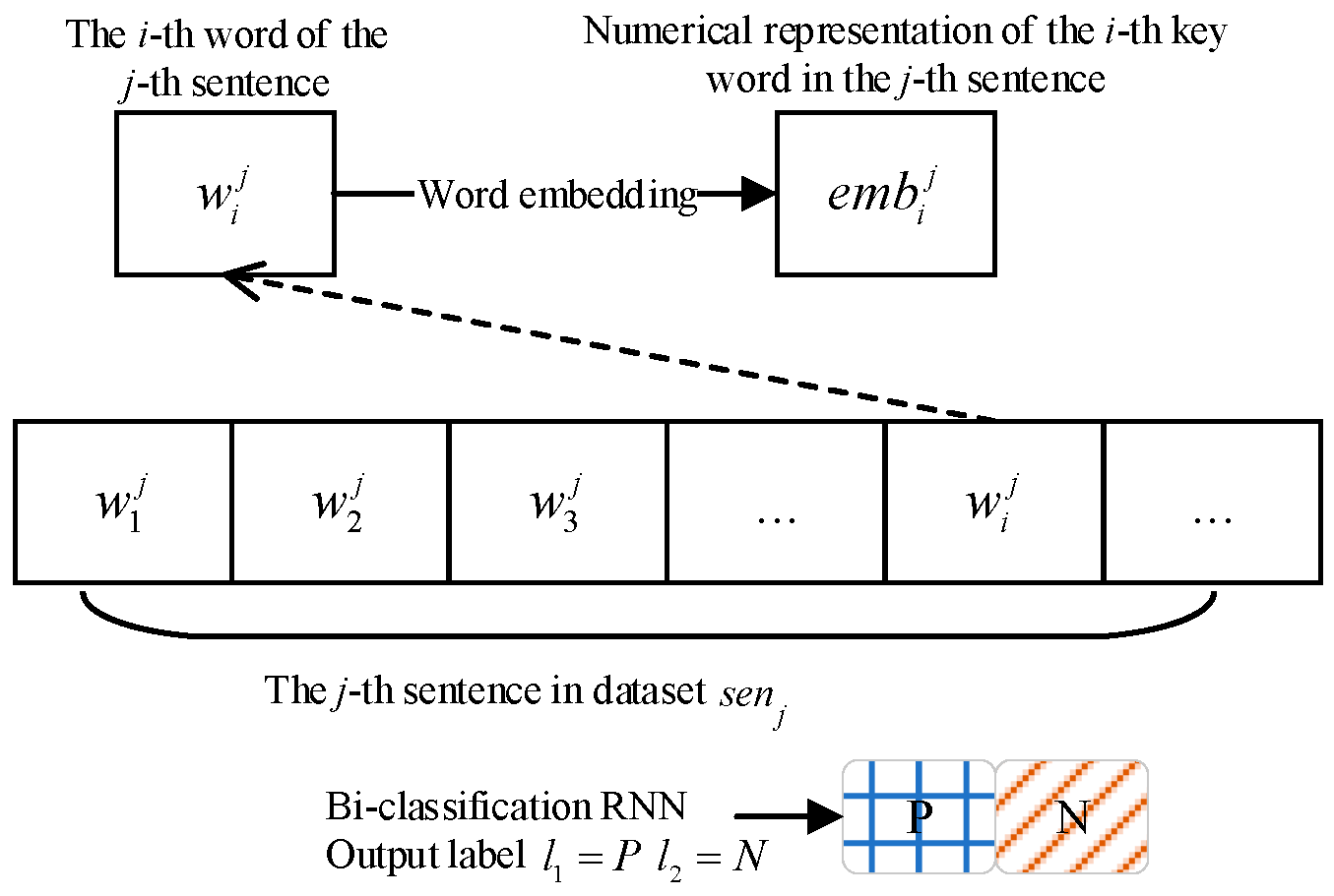
For the convenience of explaining the meaning of variables, Figure 6 shows the main variables involved in the text classification task. The variables and diagram related to RNN structure are shown in Figure 1.
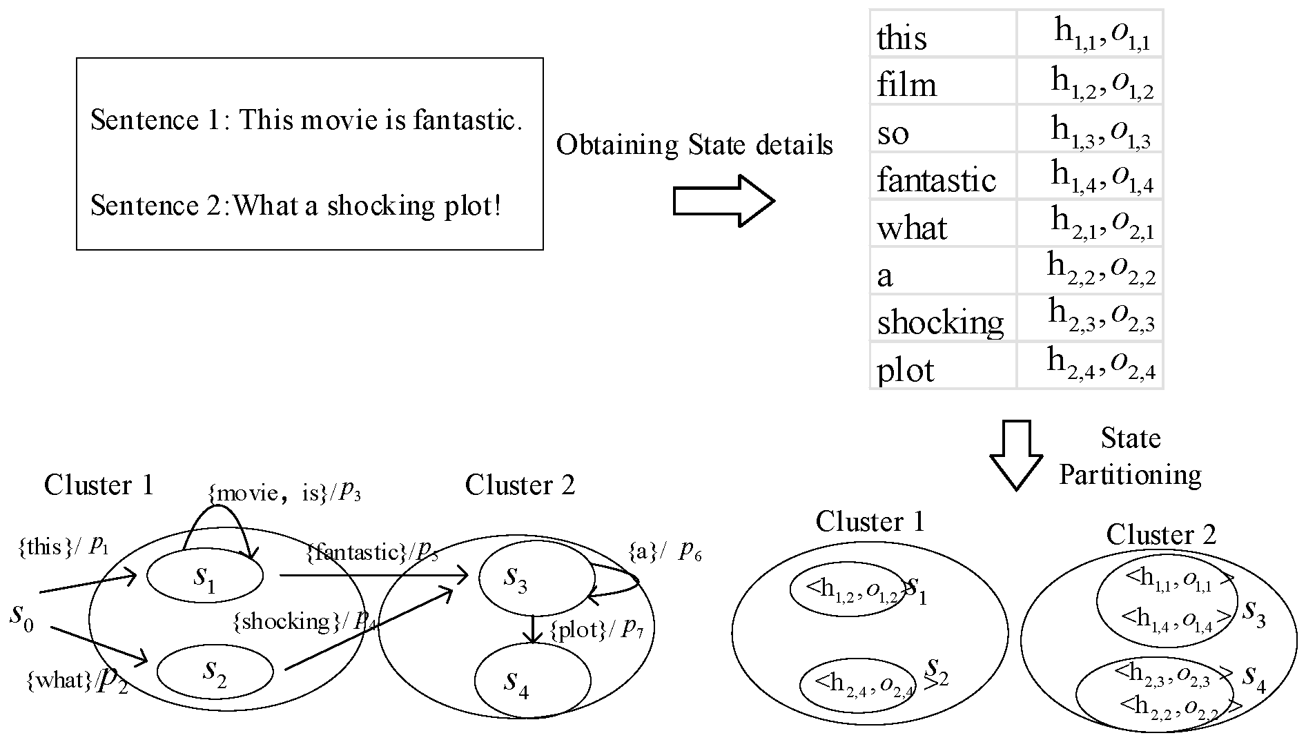
The explanation is to find the next most similar target state executed by the abstraction model when each word is inputted sequentially. In order to discover explainable features in clustering, this work proposes to use a “Compound clustering” approach for state partitioning. It is compounded by outer and inner clustering. The outer clustering C e x = { c 1 , c 2 , , c N l } is divided by the number of classification output labels, where N l is the number of labels. Each of the inner clusters c α is divided into K i n clusters, where 1 α N l . This establishes some correlations between the clustering state and the output results. The following will classify and explain input words based on PFA.
Fan et al. [18] divide the words into three categories: cross-state words, cross-cluster words, and self-pointed words. Actually, the classification result is a rough degree to which input influences output. This can be seen as a primary qualitative causal explanation. Such a word classification relies on a state machine, which assigns categories based on the behavior patterns of each word in the state machine. In other words, we only need to compare the pictures to determine the macroscopic behavior pattern of words on the state transition graph. Cross-cluster words refer to words that belong to different clusters for the current state and the next state, as shown in Figure 7, where “fantasy” and “shooting” are moved from state partition 1 to 2. These types of words can significantly alternate the classification results, which means that they can change the model’s outputs with a high probability. Cross-state words refer to words that belong to the same partition but different inner state clusters. For example, the word “plot” in Figure 7 shifts from s 3 to s 4 in the same cluster c 2 . These words may alter the confidence of predictions. Note that the first word in each sentence can be added to this group first. Self-pointed words refer to words that have the same current and referential states, such as the word “a” that jumps from s 3 to s 3 . These words often do not change much in the classification process, and their hidden state changes are relatively small after importing the RNN. The significance of explaining this classification lies in their main association with the clustering of abstract states. They reflect the external meaning of clustering to some extent.
To provide a quantitative explanation, it is also necessary to calculate the importance score of words. One is the impact of the existence of words on the probability of current prediction, that is, the change in the prediction probability of generating a specific output after inputting the word in the current step compared to the prediction probability of generating the particular output after inputting the word in the RNN before the previous step. The other is the impact of word removal on the final prediction probability. Formally, use h o l w i j and r e m w i j to represent the presence and removal of the influence of words w i j , respectively. This work uses the analysis toolkit Prism [35] to obtain quantitative attributes, such as probability from the PFA model when generating explanations.
h o l w i j = o i j α o i 1 j α
r e m w i j = p s e n j , α p s e n j \ w i j , α
They can be normalized as
h o l w i j = h o l w i j w i j s t j h o l w i j
r e m w i j = r e m w i j w i j s e n j r e m w i j
where s t j \ w i j indicates removing words w i j from the sentence s e n j . Finally, based on the weight coefficients corresponding to the words and the two influence scores above, the weight score of the words is calculated as in Equations (8) and (9), where s c o i j normalizes s c o i j . If the weight score of each word in the sentence s e n j reaches a certain threshold, the high explanation-related words are selected for the a t h output label and stored in i t p s e n j , α . This can be obtained from the sequence of high explanation-related words in the sentence. Algorithm 2 presents the specific process of explanation generation.
s c o i j = θ h o l w i j + r e m w i j
s c o i j = e i j w i j s e n j e i j
Algorithm 2. Explanation-Generating Algorithm.
Input: PFA A , text dataset D t .
Output: high-related explanation words Itp, explanation scores Sco.
  • For each sentence sen j in the text dataset D t do
  •  Obtaining word embeddings on sen j to work out the input word vector for PFA;
  •  Determine feature word classification based on behavior analysis on state
     diagram in terms of PFA
  •  Calculate the weight score of explanation words using Equations (4)–(9);
  •  If (weight score > preset threshold value) then:
  •      Add corresponding words to the set of explanation words;
  •      Record the corresponding weight score as an explanation result;
  •  EndIf
  • End for
  • Return Itp, Sco.
To understand the generation process, we give Example 4.
Example 4.
Explanation generating of sentiments classification for RNN movie reviews.
Take the sentence “This movie is nice!” as a demonstration example. The way in which it is classified as a positive label “P” will be introduced. The word embedding vector is e m b s e n = e m b 1 , e m b 2 , e m b 3 , e m b 4 , and output labels are l b   =   P . We obtain its hidden state h 1 , h 2 , h 3 , h 4 and output state o 1 , o 2 , o 3 , o 4 in the RNN. We then list all the trace paths tr from the input node to the mapped “positive” label node on PFA. The current impact probability hol and the removal impact probability rem are calculated based on Equations (4) and (5). After normalization, based on Equation (9), we can synthesize them to explain which words in the sentence have a significant impact on classification. These words, in this example, are {movie, exciting}, and then we calculate their influence score list as S c o = { ( s c o 2 , s c o 4 ) } .

4. Experimental Results

4.1. Experimental Setup

The cases in the experiment include a regular language and two text classifications. The datasets of the regular language and the movie review are publicly available online (NLP progress sentiment analysis, available online at https://nlpprogress.com/english/sentiment_analysis.html (accessed on 26 December 2023)), while the dataset of the logistics review is based on the logistics reviews of users on Amazon e-commerce platforms (Ni, J. Amazon Review Data. Available online: https://nijianmo.github.io/amazon/index.html (accessed on 28 December 2023)). The first case is the Tomita regular language classification under three artificial grammar rules. These grammar rules are used in automata learning from RNNs [21] to validate learning effectiveness. They consist of three regular languages that are defined over the alphabet {0, 1}. The grammar rules are listed in Table 1. If the string conforms to the syntax, it is marked as positive. In the experiment, training sets of different lengths for each grammar rules were created, and the length varies from 1–12 to 15–17, and the strings with lengths of 3, 11, and 16 were selected as the test set for each grammar rule. The ratio between the training and test sets is 5:1. The second case is a sentiment classification of DLRV. This dataset is extracted from customer evaluations of product logistics and is collected from comments on logistics services at Amazon e-commerce platforms. The ratio between the training and test sets is 4:1. The third case is the sentiment classification of the movie review dataset in the IMDB. The ratio between the training and testing sets is also set to 4:1.
We will measure the effectiveness and efficiency of PSO4RNN with two baseline algorithms. The first one is proposed in [17] (called BSL1 below), which uses an active learning framework to learn DFA from RNNs. The second is proposed in [25] (referred to as BSL2 hereinafter), which learns PFA from RNNs based on the AAlergia algorithm.
In the experiment, the CPU is an AMD Ryzen 7 5800H, the GPU is an Nvidia RTX 3060 Laptop with 6G video memory and Random Access Memory (RAM) with a capacity of 16G. All cases are run on a Windows 11 operating system, and the Scikit-learn toolkit is used to train RNNs. In this work, the PSO4RNN framework is implemented using Python 3.7.1. The text length of the input data they process is consistent. Each case is trained on two RNN models: a Gated Recurrent Unit (GRU) and Long Short-Term Memory (LSTM). We set the number of hidden layers for two RNNs to 1 and the dimension of the hidden state to 508. In the training process, a One-Hot encoding technique is applied to encode characters in the Tomita dataset, and word2vec is used for text classification to convert each word in the real natural language into a 288-dimensional numerical vector.

4.2. Results

4.2.1. Effectiveness

This work is compared with BSL1 and BSL2 with regard to the accuracy and efficiency of the abstraction model.
(1) Accuracy of the abstraction model. The accuracy is the proportion of the number of samples on the training set, and they are the samples of which the RNN outputs approximate to its PFA. They can be calculated by a c c = Σ x D T r s i g n A x R x D T r , where D T r represents the samples in training datasets and D T r is its total number of samples. A is the learned model, R is the target RNN, and T is the testing set of sentences. s i g n A x R x indicates whether the RNN and PFA perform approximating behavior on sample x. There are three datasets in this work, among which the accuracy of Tomita syntax was taken as the mean of the three grammar rules. Classifiers are trained for different tasks on two types of RNNs; so, we create six models for these datasets. In order to scientifically and systematically compare with BSL1 and BSL2, the k-means algorithm is used in all experiments for state partitioning. The number of clusters is fixed to 18. Figure 8 shows a comparison of accuracy for six models under three abstracting techniques.
It can be observed that the models learned by PSO4RNN are significantly more accurate than those generated by BSL1 and BLS2. PSO4RNN usually maintains an accuracy of 80% to nearly 95%, while the accuracy of BSL1 ranges from 50% to slightly above 90%. The accuracy error between the model learned by PSO4RNN and the original RNN model fluctuates within the range of 10%. This indicates that PSO4RNN approaches the behavior of RNNs at a satisfying accuracy. As is shown in Figure 8, the accuracy of PSO4RNN is also slightly higher than that of BSL2. This is partly because the PD-PSO searches for a proper generalization score of PFA instead of the golden section search in BSL2.
(2) Restoration degree of the abstraction model. If the behavior in PFA is consistent with the RNN, it indicates that they share similarities in testing datasets. Due to the inevitable loss of information details in abstraction, it is impossible to 100% replicate the behavior of the RNN. Therefore, the similarity must be examined after model abstraction. The corresponding metric of similarity is the model restoration degree: R e = Σ x T s i g n A x R x T , where A is the learned model, R is the target RNN, and T is the testing set of sentences. s i g n A x R x indicates whether the RNN and PFA perform approximating behavior on sample x. The restoration degree obtained from different models is shown in Table 2.
(3) The abstraction error curve: The abstraction error is defined as the difference between the predicted results on DFA/PFA and the RNN on the training samples. During the experiment, three model abstraction techniques were trained twenty times on the DLRV dataset, and the average error was calculated for all iterations. The curve of their abstraction error is shown in Figure 9. It is an error reduction curve, as it has been normalized.
According to the error curve, it can be seen that when a specific low error value is reached, PSO4RNN has the least number of iterations, and the actual training time is also relatively short. The time consumption is shown in Table 3, which is calculated by averaging eight repeated experiments. All methods are set to 10 clusters in the state clustering process, and the time consumption is how long it takes to learn an automaton at an abstraction error of less than 0.4.
From the statistical results, it can be seen that after ensuring sufficient accuracy for the level of abstraction, PSO4RNN has the lowest time consumption in abstract learning compared to BSL1 and BSL2. This is because the PSO algorithm improves the search efficiency in the learning process of PFA.
(4) Space complexity of the abstraction model. This metric refers to the scale of storage cost by the learned model PFA/DFA. In practical situations, the abstraction model can be represented by an adjacency matrix. Intuitively speaking, the fewer states and edges there are, the lower its complexity. After adjusting the number of clusters and making their abstraction errors below 0.4, we counted the total number of states in the six abstraction models. Table 4 shows the number of states obtained from different abstraction techniques on the IMDB sentiment dataset.
It can be seen that, while ensuring an abstraction error below 0.4, the scale of the abstract model is much smaller than the RNN model. PSO4RNN requires fewer state nodes to keep the behavior of the original RNN. This also indicates that the probabilistic model learned by PSO4RNN is more general, and its abstraction effect is more competitive. DFA learned by BSL1 has a higher number of states because DFA lacks information on probability distribution.

4.2.2. Usefulness

(1)
Explanation Generating
Based on the explanation of PSO4RNN, word clouds and word highlighting are used to visualize the explanation. As shown in Figure 10, a word cloud of the DLRV dataset is calculated from the word frequency under each word category. The font size of a word reflects the appearance frequency in this dataset.
Here are the explanation examples in Figure 11 and Figure 12. The explanation words are highlighted in the sentences of the DLRV and IMDB datasets. The scores under each word are the explanation importance calculated by Algorithm 2.
In Figure 11 and Figure 12, the gray words correspond to self-pointed words, which hardly affect sentiment classification. The blue words correspond to cross-state words, and they do not significantly affect sentiment classification. The red words correspond to cross-cluster words, which influence the sentiment classification. It is not difficult to see that the highlighted words conform to human cognition. That is, cross-cluster words can convey and influence the emotions of the sentence. Through experiments on other texts, we found that this rationality is very common, which can effectively promote human understanding of the cause of the decision making of an RNN. Compared to directly generating explanations on the RNN model, generating explanations by PSO4RNN is faster and reduces the cost of accessing the model. In addition, visualization techniques, such as the word cloud and the highlight explanation, make the explanation intuitive.
(2)
Adversarial Text Detection
Compared to the image field, research on adversarial attacks in the text field remains to be expanded. In addition, the highly discrete nature of text content is different from the pixels of images, which makes it challenging to transfer image adversarial attacks to the one of texts. Adversarial attacks can expose the fragility of machine learning models, which will help to analyze the robustness, especially the explainability of RNNs [36,37]. Identifying and deleting adversarial samples can prevent the generation of adversarial patterns and alleviate adversarial attacks. Abstraction models can be used for adversarial text detection. It has been shown in [38] that adversarial text can be automatically generated by perturbating slightly on non-poisoned text. Typical techniques for generating adversarial text include replacing words with synonyms and using machine learning models to translate sentences multiple times (e.g., from English to Spanish and then back to English).
Inspired by Dong et al.’s work [25], this work uses Equation (10) to describe the adversarial text detection ratio. Given a sentence x, the adversarial text detection ratio can be defined as follows:
T x , y = P x , y P x , y ¯
where y is the output label predicted by the RNN and P(x, y) is the probability from input x to output y on PFA. P x ,   y ¯ represents the total probability of reaching outputs other than y from input x. We use the stochastic model checking tool Prism [35] to compute the probability. We select a threshold T θ for comparison with T(x, y), which can serve as a critical value for distinguishing adversarial text from benign text. If the text’s T(x, y) is less than T θ , it is considered an adversarial text.
Example 5.
Simple Adversarial Text Detection Case.
Let us consider the sentence and PFA in Example 1. Assuming x = “This movie is so beautiful!” and y = P, y ¯ = N. T θ is set as 3. The input that passes through the trace to label P is s 1 s 3 s 3 s 4 . Then, its probability in Equation (10) is P x , y = t r s 1 , s 3 t r s 3 , s 3 t r s 3 , s 4 = 0.2430, where tr(s, s’) means transition probability from s to s’. P(x, y ¯ ) = t r s 1 , s 3 t r s 3 , s 3   t r s 3 , s 5 = 0.0675. According to Equation (10), T(x, y) = 3.6. If it is greater than T θ , then x is not an adversarial text.
Assume there are N b n benign samples and N p n samples with poisoning attacks. There are four modes selected for poisoning: (1) insertion, (2) change, (3) delete, and (4) order swapping. The first step of adversarial text detection is to learn PFA from RNNs. Secondly, the poisoned sentence x’ is input into PFA, and the probability P(x’, y) is calculated based on PFA. Thirdly, a clean sequence x is input into PFA, and we calculate P(x, y). Finally, in Equation (10), the sentences that have a lower ratio T(x, y) than the threshold are identified as adversarial text. For all adversarial samples, if one of them is detected as benign text, it fails to detect real adversarial text. We set the number of samples correctly detected as n u m c d , and then detection accuracy can be defined as A c c a d = n u m c d / N b n . Figure 13 provides an overview of this detection effect evaluation process.
The detection accuracy MSE is the average of A c c a d in ten experiments. The A c c a d MSE of PSO4RNN on three datasets is shown in Table 5. Here, LSTM is an RNN with one hidden layer and 508 hidden nodes, and the number of state clusters is 12.
This result demonstrates that the abstraction technique in PSO4RNN ensures high detection accuracy. It has practical significance in mitigating adversarial text attack scenarios, helping to detect adversarial patterns efficiently. The model learning approach not only provides a way to understand how the RNN works but also has the potential to open the door to applying software analysis techniques (such as model-based testing, model checking, runtime monitoring, and validation) to real-world RNN models.

5. Discussion

The accuracy of the abstraction model indicates how an abstraction model approaches the behavior of RNNs. In Figure 8, it is evident that PSO4RNN performs better than BSL1. This is partly because the model learned by BSL1 only contains state transitions with maximum frequency, while PSO4RNN can preserve almost all state transitions through probability distribution. In addition, it can be observed that BSL2 uses unpropertied parameters to merge FPT in most cases. The complexity metric answers how many resources the learned model takes to mimic an RNN. Remarkably, abstraction models learned by PSO4RNN are the most straightforward.
The restoration degree indicates how a model keeps the original RNN patterns on the testing set. It stands for the generalizing ability of an abstraction model. PSO4RNN performs much better in generalizing than BSL1 and BSL2. This means that PSO4RNN learned more effective rules when analyzing unknown data. This might be attributed to the random strategy of PSO4RNN to search for BIC parameters. For the abstraction error curve and time consumption results, PSO4RNN shows the most efficient technique for learning from an RNN. Because BSL1 takes a lot of time to execute requirements from an RNN, it needs to maintain a huge observation table. BSL2 is also weaker than PSO4RNN because BSL2 applies a trial-and-error strategy to learn PFA from the RNN. In contrast, PSO4RNN uses PSO to search BIC parameters. It does not require testing all possible BIC parameters from a wide range. Guided by fitness, it can self-adaptively update these parameters towards a clearer goal.
Concerning the usefulness of explanation, this work provides two forms tailored for different users: qualitative results and quantitative scores. Common users can directly, according to the color, discriminate the importance of features. Professional researchers may need a quantitative score to analyze in their subsequent studies. In part (2) of Section 4.2.2, we introduce a text adversarial case to prove the usefulness of learned PFA. The usefulness study of this work shows that such a quantitative explanation can serve well in real-world tasks.
Based on the experimental analysis, it can be found that the performance of different techniques varies because of their advantages and disadvantages. The comparisons are compiled in Table 6, which offers a clear and systematic evaluation.

6. Conclusions and Future Works

6.1. Conclusions

This paper proposes a PSO-based model abstraction and explanation generation method for RNNs. This work presents three primary novel contributions as follows:
  • Learning PFA to integrate the information into the abstraction model;
  • Adding PSO module to optimize the state merging algorithm;
  • Abstracting RNN models to simplify the research of explainability;
Compared with the existing RNN abstraction techniques, it performs better in model accuracy and running efficiency. PSO4RNN optimizes the parameter search instead of trial and error, providing a novel technical perspective for the application of heuristic algorithms in state merging. The abstraction provides a novel perspective for explainable artificial intelligence (XAI). Existing works learned the abstraction model a global structure explanation. Moreover, it generates high-related explanation words and their importance scores based on PFA, which can be seen as a well-adapted global explanation. This adaptability mainly comes from the good generalization performance of abstraction model PFA, not only in training set samples. It also provides visualization ways, such as word clouds and feature word highlighting, to increase explainability, greatly enhancing the user friendliness and credibility of abstraction models.
However, this work has several limitations. (1) Restricted by hardware resources, empirical studies are merely investigated on two real-world datasets. The clustering parameter k is selected through haphazard tests. If PSO4RNN is applied to other real-world datasets containing many more samples, the clustering process may not perform optimally. Therefore, choosing a proper k to achieve a satisfying performance becomes meaningful. (2) Computational efficiency can be improved. During experiments, an issue of inadequate computational resources appeared in the state merging process. This means that the throughput of merging processing needs enhancement.

6.2. Future Works

In PSO4RNN, the k-means is used to extract abstract state traces. Selecting a proper number of clusters is not automatic. Therefore, combining other clustering algorithms, such as the DBSCAN or GMM models, is a promising way to overcome this limitation. We will design such a combination in the subsequent works. There is still room for improving computational efficiency in state merging. Parallel or distributed learning strategies also help improve. This will remain to be implemented in future works.
The future work will implement learning the abstraction model at runtime, which can further adaptively compress the state space of the abstraction model. This will be our main future work. A reinforcement learning (RL) method can be promising in abstracting at runtime. Real-world runtime problems usually involve interacting with the dynamic environment, while RL is suitable for solving these problems.
In addition, we aim to shift the abstraction of RNNs from specialized to universally applicable tasks. Empirical research will be conducted on larger-scale pre-trained models, including the most prevalent large-scale language models

Author Contributions

Conceptualization, Y.L. and H.W.; methodology, Y.L.; software, H.W.; validation, Y.L. and H.W.; investigation, Y.L. and Y.M.; resources, H.W.; data curation, H.W.; writing—original draft preparation, Y.L. and H.W.; writing—review and editing, Y.L. and Y.M.; visualization, H.W.; supervision, Y.L. and Y.M.; project administration, Y.L.; funding acquisition, Y.L. All authors have read and agreed to the published version of the manuscript.

Funding

This research was funded by MOE Humanities and the Social Sciences Foundation of China under Grant No. 20YJCZH102 and Singapore–UK Cyber Security of EPSRC under Grant No. EP/N020170/1.

Institutional Review Board Statement

Not applicable.

Informed Consent Statement

Not applicable.

Data Availability Statement

The original contributions presented in the study are included in the article, further inquiries can be directed to the corresponding author/s.

Conflicts of Interest

The authors declare no conflicts of interest.

References

  1. Yüksel, N.; Börklü, H.R.; Sezer, H.K.; Canyurt, O.E. Review of artificial intelligence applications in engineering design perspective. Eng. Appl. Artif. Intell. 2023, 118, 105697. [Google Scholar] [CrossRef]
  2. Zhang, S.; Wu, L.; Yu, S.G.; Shi, E.Z.; Qiang, N.; Gao, H.; Zhao, J.Y.; Zhao, S.J. An Explainable and Generalizable Recurrent Neural Network Approach for Differentiating Human Brain States on EEG Dataset. Ieee Trans. Neural Netw. Learn. Syst. 2022. Article ASAP. [Google Scholar] [CrossRef]
  3. Chang, G.; Gao, H.; Yao, Z.; Xiong, H. TextGuise: Adaptive adversarial example attacks on text classification model. Neurocomputing 2023, 529, 190–203. [Google Scholar] [CrossRef]
  4. Kapil, P.; Ekbal, A. A deep neural network based multi-task learning approach to hate speech detection. Knowl.-Based Syst. 2020, 210, 106458. [Google Scholar] [CrossRef]
  5. Peng, X.; Xian, H.; Lu, Q.; Lu, X. Semantics aware adversarial malware examples generation for black-box attacks. Appl. Soft Comput. 2021, 109, 107506. [Google Scholar] [CrossRef]
  6. Du, M.; Liu, N.; Yang, F.; Ji, S.; Hu, X. On Attribution of Recurrent Neural Network Predictions via Additive Decomposition. In Proceedings of the The World Wide Web Conference, San Francisco, CA, USA, 13–17 May 2019; pp. 383–393. [Google Scholar]
  7. Li, X.Z.; Lin, F.F.; Wang, H.; Zhang, X.; Ma, H.; Wen, C.Y.; Blaabjerg, F. Temporal Modeling for Power Converters with Physics-in-Architecture Recurrent Neural Network. Ieee Trans. Ind. Electron. 2024. Article ASAP. [Google Scholar] [CrossRef]
  8. Chen, W.T.; Zhang, W.E.; Yue, L. Death comes but why: A multi-task memory-fused prediction for accurate and explainable illness severity in ICUs. World Wide Web-Internet Web Inf. Syst. 2023, 26, 4025–4045. [Google Scholar] [CrossRef]
  9. Barredo Arrieta, A.; Díaz-Rodríguez, N.; Del Ser, J.; Bennetot, A.; Tabik, S.; Barbado, A.; Garcia, S.; Gil-Lopez, S.; Molina, D.; Benjamins, R.; et al. Explainable Artificial Intelligence (XAI): Concepts, taxonomies, opportunities and challenges toward responsible AI. Inf. Fusion 2020, 58, 82–115. [Google Scholar] [CrossRef]
  10. Yang, C.; Zhou, W.X.; Wang, Z.Y.; Jiang, B.; Li, D.S.; Shen, H.W. Accurate and Explainable Recommendation via Hierarchical Attention Network Oriented towards Crowd Intelligence. Knowl.-Based Syst. 2021, 213, 106687. [Google Scholar] [CrossRef]
  11. Hong, D.; Segre, A.M.; Wang, T. AdaAX: Explaining Recurrent Neural Networks by Learning Automata with Adaptive States. In Proceedings of the 28th ACM SIGKDD Conference on Knowledge Discovery and Data Mining, Washington DC, USA, 14–18 August 2022; pp. 574–584. [Google Scholar]
  12. Yang, M.; Moon, J.; Yang, S.; Oh, H.; Lee, S.; Kim, Y.; Jeong, J. Design and Implementation of an Explainable Bidirectional LSTM Model Based on Transition System Approach for Cooperative AI-Workers. Appl. Sci. 2022, 12, 6390. [Google Scholar] [CrossRef]
  13. Khmelnitsky, I.; Neider, D.; Roy, R.; Xie, X.; Barbot, B.; Bollig, B.; Finkel, A.; Haddad, S.; Leucker, M.; Ye, L. Analysis of recurrent neural networks via property-directed verification of surrogate models. Int. J. Softw. Tools Technol. Transf. 2023, 25, 341–354. [Google Scholar] [CrossRef]
  14. Guillaumier, K.; Abela, J. Learning DFAs by Evolving Short Sequences of Merges. In Proceedings of the ICGI 2021—15th International Conference on Grammatical Inference, Virtual/New York City, NY, USA, 23 August 2021; pp. 217–236. [Google Scholar]
  15. Angluin, D. Learning regular sets from queries and counterexamples. Inf. Comput. 1987, 75, 87–106. [Google Scholar] [CrossRef]
  16. Vaandrager, F. Model learning. Commun. ACM 2017, 60, 86–95. [Google Scholar] [CrossRef]
  17. Hou, B.J.; Zhou, Z.H. Learning With Interpretable Structure From Gated RNN. IEEE Trans. Neural Netw. Learn. Syst. 2020, 31, 2267–2279. [Google Scholar] [CrossRef]
  18. Fan, M.; Si, Z.; Xie, X.; Liu, Y.; Liu, T. Text Backdoor Detection Using an Interpretable RNN Abstract Model. IEEE Trans. Inf. Forensics Secur. 2021, 16, 4117–4132. [Google Scholar] [CrossRef]
  19. Wei, Z.; Zhang, X.; Zhang, Y.; Sun, M. Weighted automata extraction and explanation of recurrent neural networks for natural language tasks. J. Log. Algebr. Methods Program. 2024, 136, 100907. [Google Scholar] [CrossRef]
  20. Yellin, D.M.; Weiss, G. Synthesizing Context-free Grammars from Recurrent Neural Networks. In Proceedings of the Tools and Algorithms for the Construction and Analysis of Systems, TACAS 2021, Luxembourg City, Luxembourg, 27 March–1 April 2021; Springer: Cham, Switzerland, 2021; pp. 351–369. [Google Scholar]
  21. Weiss, G.; Goldberg, Y.; Yahav, E. Extracting Automata from Recurrent Neural Networks Using Queries and Counterexamples. In Proceedings of the 35th International Conference on Machine Learning, Stockholm, Sweden, 10–15 July 2018; Proceedings of Machine Learning Research; pp. 5247–5256.
  22. Barbot, B.; Bollig, B.; Finkel, A.; Haddad, S.; Khmelnitsky, I.; Leucker, M.; Neider, D.; Roy, R.; Ye, L. Extracting Context-Free Grammars from Recurrent Neural Networks using Tree-Automata Learning and A* Search. In Proceedings of the ICGI 2021—15th International Conference on Grammatical Inference, Virtual/New York City, NY, USA, 23 August 2021; pp. 113–129. [Google Scholar]
  23. Wang, J.; Sun, J.; Yuan, Q.; Pang, J. Learning probabilistic models for model checking: An evolutionary approach and an empirical study. Int. J. Softw. Tools Technol. Transf. 2018, 20, 689–704. [Google Scholar] [CrossRef]
  24. Weiss, G.; Goldberg, Y.; Yahav, E. Learning deterministic weighted automata with queries and counterexamples. In Proceedings of the 33rd International Conference on Neural Information Processing Systems, Vancouver, BC, Canada, 8–14 December 2019; Weiss, G., Goldberg, Y., Yahav, E., Eds.; Curran Associates Inc.: New York City, NY, USA, 2019; pp. 8560–8571. [Google Scholar]
  25. Dong, G.; Wang, J.; Sun, J.; Zhang, Y.; Wang, X.; Dai, T.; Dong, J.S.; Wang, X. Towards interpreting recurrent neural networks through probabilistic abstraction. In Proceedings of the 35th IEEE/ACM International Conference on Automated Software Engineering, Virtual Event, 21–25 December 2021; pp. 499–510. [Google Scholar]
  26. Mao, H.; Chen, Y.; Jaeger, M.; Nielsen, T.D.; Larsen, K.G.; Nielsen, B. Learning Probabilistic Automata for Model Checking. In Proceedings of the 2011 Eighth International Conference on Quantitative Evaluation of SysTems, Aachen, Germany, 5–8 September 2011; pp. 111–120. [Google Scholar]
  27. Bhattacharya, C.; Ray, A. Thresholdless Classification of chaotic dynamics and combustion instability via probabilistic finite state automata. Mech. Syst. Signal Process. 2022, 164, 108213. [Google Scholar] [CrossRef]
  28. Ishimoto, Y.; Kondo, M.; Ubayashi, N.; Kamei, Y. PAFL: Probabilistic Automaton-Based Fault Localization for Recurrent Neural Networks. Inf. Softw. Technol. 2023, 155, 107117. [Google Scholar] [CrossRef]
  29. Wang, Q.; Zhang, K.; Ororbia, A.G., II; Xing, X.; Liu, X.; Giles, C.L. An Empirical Evaluation of Rule Extraction from Recurrent Neural Networks. Neural Comput. 2018, 30, 2568–2591. [Google Scholar] [CrossRef]
  30. Carr, S.; Jansen, N.; Topcu, U. Task-Aware Verifiable RNN-Based Policies for Partially Observable Markov Decision Processes. J. Artif. Intell. Res. 2021, 72, 819–847. [Google Scholar] [CrossRef]
  31. Wang, C.; Lawrence, C.; Niepert, M. State-Regularized Recurrent Neural Networks to Extract Automata and Explain Predictions. Ieee Trans. Pattern Anal. Mach. Intell. 2023, 45, 7739–7750. [Google Scholar] [CrossRef]
  32. Du, X.; Xie, X.; Li, Y.; Ma, L.; Liu, Y.; Zhao, J. DeepStellar: Model-based quantitative analysis of stateful deep learning systems. In Proceedings of the 2019 27th ACM Joint Meeting on European Software Engineering Conference and Symposium on the Foundations of Software Engineering, Tallinn, Estonia, 26–30 August 2019; pp. 477–487. [Google Scholar]
  33. Maes, P. Concepts and experiments in computational reflection. In Proceedings of the Conference Proceedings on Object-Oriented Programming Systems, Languages and Applications, Orlando, FL, USA, 4–8 October 1987; pp. 147–155. [Google Scholar]
  34. Vouros, G. Explainable Deep Reinforcement Learning: State of the Art and Challenges. ACM Comput. Surv. 2023, 55, 92. [Google Scholar] [CrossRef]
  35. Kwiatkowska, M.; Norman, G.; Parker, D. PRISM 4.0: Verification of Probabilistic Real-Time Systems. In Proceedings of the International Conference on Computer Aided Verification, CAV 2011, Snowbird, UT, USA, 14–20 July 2011; Springer: Berlin/Heidelberg, Germany, 2011; pp. 585–591. [Google Scholar]
  36. Chen, C.; Dai, J. Mitigating backdoor attacks in LSTM-based text classification systems by Backdoor Keyword Identification. Neurocomputing 2021, 452, 253–262. [Google Scholar] [CrossRef]
  37. Wang, B.; Yao, Y.; Shan, S.; Li, H.; Viswanath, B.; Zheng, H.; Zhao, B.Y. Neural Cleanse: Identifying and Mitigating Backdoor Attacks in Neural Networks. In Proceedings of the 2019 IEEE Symposium on Security and Privacy (SP), San Francisco, CA, USA, 19–23 May 2019; pp. 707–723. [Google Scholar]
  38. Li, J.; Ji, S.; Du, T.; Li, B.; Wang, T. TextBugger: Generating Adversarial Text Against Real-World Applications. arXiv 2018, arXiv:1812.05271. [Google Scholar]
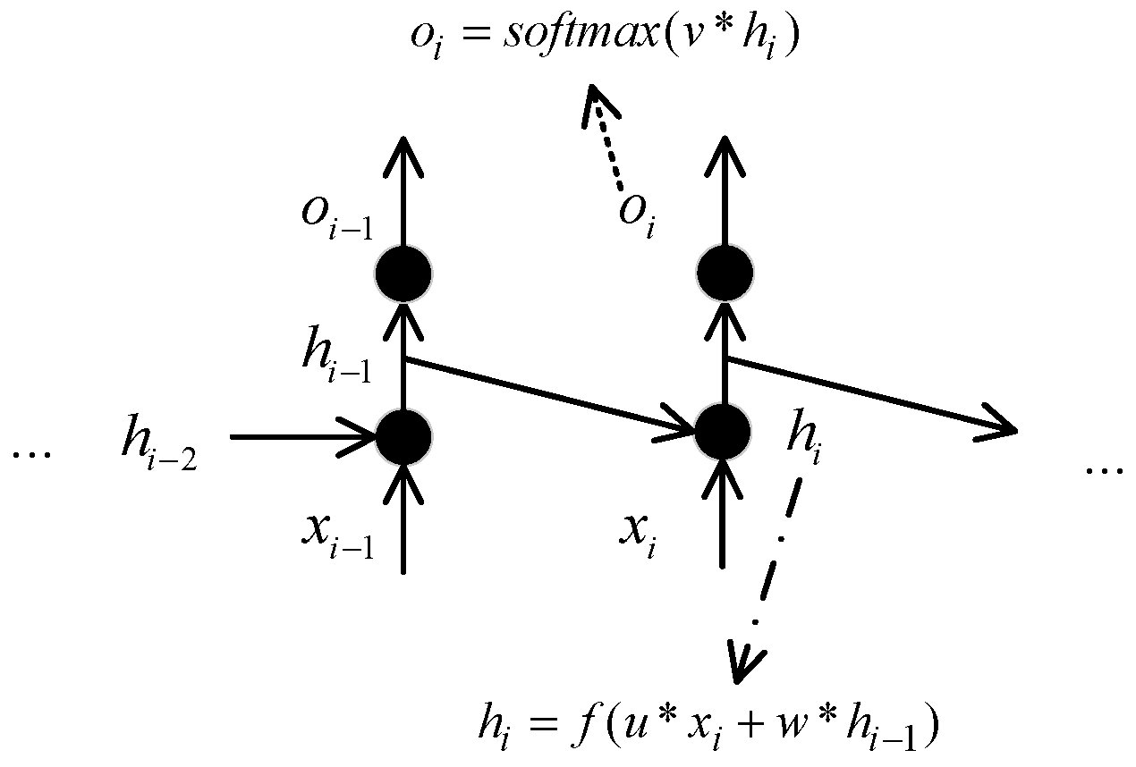
Figure 1. RNN basic unit.
Algorithms 17 00210 g001
Figure 3. PSO4RNN framework.
Algorithms 17 00210 g003
Figure 4. Abstract state trace in Example 2.
Algorithms 17 00210 g004
Figure 5. Example of a frequency prefix tree.
Algorithms 17 00210 g005
Figure 6. Meanings of the main variables in the text classification process.
Algorithms 17 00210 g006
Figure 7. State partitioning of two sentences.
Algorithms 17 00210 g007
Figure 8. Accuracy of different abstraction models on the training sets.
Algorithms 17 00210 g008
Figure 9. Error change curves of three models.
Algorithms 17 00210 g009
Figure 10. Word cloud of cross-cluster words, cross-state words, and self-pointed words in the DLRV dataset. Subfigure (a) corresponds to the word cloud of the cross-cluster words, Subfigure (b) corresponds to the word cloud of the cross-state words, and Subfigure (c) corresponds to the word cloud of the self-pointed words.
Algorithms 17 00210 g010
Figure 11. Explanation of Highlighted Keywords on DLRV. Sentences (ac) are text samples in DLRV. The gray words correspond to self-pointed words. The blue words correspond to cross-state words. The red words correspond to cross-cluster words.
Algorithms 17 00210 g011
Figure 12. Explanation of highlighted keywords in the IMDB. Sentences (ac) are text samples in IMDB. The gray words correspond to self-pointed words. The blue words correspond to cross-state words. The red words correspond to cross-cluster words.
Algorithms 17 00210 g012
Figure 13. Adversarial text detection evaluation process.
Algorithms 17 00210 g013
Table 1. Three Tomita artificial grammar rules.
GrammarDescription
Tomita_11*
Tomita_2(10)*
Tomita_3Compliments of ((0|1)* 0)*1(11)*(0(0|1)*1)*0(00)*(1(0|1)*)*
Note: In regular expressions, the asterisk (*) is a quantifier used to specify that the preceding expression can be repeated zero or more times.
Table 2. Classification restoration degree of the original model on the test datasets.
Abstracting TechniqueIMDB-ReDLRV-ReTomita-Re
BSL10.430.390.62
BSL20.460.360.65
PSO4RNN0.670.470.83
Table 3. Time consumption of the three techniques for LSTM abstraction learning.
Time Consumption BSL1 BSL2PSO4RNN
Tomita-LSTM0.23 h0.12 h0.11 h
IMDB-LSTM0.34 h0.17 h0.13 h
DLRV-LSTM0.37 h0.23 h0.21 h
Note: the unit of time cost is hours (h).
Table 4. The number of states abstracted from different models.
Technique TypeState Numbers
BSL1 on GRU text sentiment analysis37
BSL1 on LSTM text sentiment analysis43
BSL2 on GRU text sentiment analysis25
BSL2 on LSTM text sentiment analysis31
PSO4RNN on GRU text sentiment analysis22
PSO4RNN on LSTM text sentiment analysis28
Table 5. Adversarial text detection accuracy based on PSO4RNN.
DatasetAdversarial Sample Detection Accuracy MSE
Tomita93%
IMDB92%
DLRV89%
Table 6. Characteristics comparison of this work and existing techniques.
CharacteristicsBSL1BSL2PSO4RNN
RNN structure explanationyesyesyes
Feature importance explanationnonoyes
Probabilistic informationnot consideredyesyes
BIC parameter searching methodnonetrial and errorheuristic
Note: Row 1 in Table 6 shows whether the technique provides an explanation of the global structure of the RNN. Row 2 means whether the technique provides a quantitative explanation of features. Row 3 means whether the learned model considers the probabilistic information. Row 4 indicates the method used in the searching process.
Disclaimer/Publisher’s Note: The statements, opinions and data contained in all publications are solely those of the individual author(s) and contributor(s) and not of MDPI and/or the editor(s). MDPI and/or the editor(s) disclaim responsibility for any injury to people or property resulting from any ideas, methods, instructions or products referred to in the content.