Article

Three-Way Alignment Improves Multiple Sequence Alignment of Highly Diverged Sequences

1
Department of Biology, University of Ottawa, 30 Marie Curie, P.O. Box 450, Ottawa, ON K1N 6N5, Canada
2
Ottawa Institute of Systems Biology, Ottawa, ON K1H 8M5, Canada
*
Author to whom correspondence should be addressed.
Algorithms 2024, 17(5), 205; https://doi.org/10.3390/a17050205
Submission received: 25 March 2024 / Revised: 2 May 2024 / Accepted: 8 May 2024 / Published: 10 May 2024
(This article belongs to the Special Issue Advanced Research on Machine Learning Algorithms in Bioinformatics)

Abstract

:
The standard approach for constructing a phylogenetic tree from a set of sequences consists of two key stages. First, a multiple sequence alignment (MSA) of the sequences is computed. The aligned data are then used to reconstruct the phylogenetic tree. The accuracy of the resulting tree heavily relies on the quality of the MSA. The quality of the popularly used progressive sequence alignment depends on a guide tree, which determines the order of aligning sequences. Most MSA methods use pairwise comparisons to generate a distance matrix and reconstruct the guide tree. However, when dealing with highly diverged sequences, constructing a good guide tree is challenging. In this work, we propose an alternative approach using three-way dynamic programming alignment to generate the distance matrix and the guide tree. This three-way alignment incorporates information from additional sequences to compute evolutionary distances more accurately. Using simulated datasets on two symmetric and asymmetric trees, we compared MAFFT with its default guide tree with MAFFT with a guide tree produced using the three-way alignment. We found that (1) the three-way alignment can reconstruct better guide trees than those from the most accurate options of MAFFT, and (2) the better guide tree, on average, leads to more accurate phylogenetic reconstruction. However, the improvement over the L-INS-i option of MAFFT is small, attesting to the excellence of the alignment quality of MAFFT. Surprisingly, the two criteria for choosing the best MSA (phylogenetic accuracy and sum-of-pair score) conflict with each other.

1. Introduction

Inferring evolutionary relationships among various species from molecular data, such as protein, DNA, and RNA sequences, is a basic problem in evolutionary biology. Multiple sequence alignment (MSA) is a primary step in phylogenetic reconstruction, and the accuracy of MSA directly affects the accuracy of reconstructing a phylogeny, especially a deep phylogeny [1,2,3,4].
The most common method for aligning two sequences (pairwise sequence alignment, or PSA) is the Needleman–Wunsch algorithm [5], which is a dynamic programming (DP) approach that finds the optimal alignment based on a given scoring scheme [6,7,8]. Using DP in PSA is feasible in quadratic time and memory, which can even be reduced to linear memory requirement [9]. The idea of using DP for sequence alignment can be easily extended to MSA. However, multi-dimensional DP is practically infeasible even for a small number of sequences, due to time and space complexity [10].
As an alternative, a progressive alignment approach was proposed for MSA [11] and implemented in many alignment tools, such as MAFFT [12], MUSCLE [13], T-COFFEE [14], and CLUSTAL-W [15]. Progressive alignment fundamentally simplifies the task of MSA by breaking it down into a series of pairwise and profile alignments. Progressive alignment involves constructing a guide tree to determine the order of aligning sequences and performing pairwise and profile alignment from the leaves of the guide tree to the root. The guide tree is usually constructed by using distance-based methods like UPGMA and neighbor joining (NJ) from a distance matrix obtained mainly from (1) k-tuple similarity or (2) PSA.
Current MSA methods and tools perform well on aligning closely related sequences [16]. However, the performance of these methods decreases with sequence divergence [17,18,19]. Virtually everyone interested in deep phylogeny is looking for ways to improve MSA. Some have incorporated secondary structure to guide the sequence alignment [20,21,22,23], while others explored post-alignment refinement [1,17]. The improvement of MSA with these approaches remains limited.
A guide tree is a crucial component in progressive alignment, and its accuracy affects the accuracy of output alignment [24]. A few studies have shown that an inaccurate guide tree could be a major source of error in progressive sequence alignment [25,26]. Therefore, different strategies for improving guide trees have been proposed [24]. Two criteria have been used to evaluate the effect of guide trees on the accuracy of MSA generated by MAFFT and ClustalW, including (1) the sum-of-pair score (SPS), excluding shared gaps in pairwise comparisons, and (2) the accuracy of phylogenetic reconstruction [27,28]. The result indicates that the final SPS is affected little by the initial guide tree, but better guide trees significantly improve the accuracy of the reconstructed phylogenies.
However, constructing an accurate guide tree is difficult for highly diverged sequences. Aligning three sequences using dynamic programming is expected to improve the alignment and, in particular, the estimated distances used to build the initial guide tree [14,15,29,30].
Three-dimensional dynamic programming (3D_DP), as formulated by Gotoh [31], represents an extension of the Needleman–Wunsch algorithm originally proposed for pairwise sequence alignment. Gotoh contributed to developing 3D-DP for an affine gap penalty. His approach to 3D-DP increases the time and space requirements to cubic complexity, which is not feasible for long sequences. The Carrillo–Lipman [32] algorithm was proposed to narrow down the search space within N-dimensional dynamic programming. The idea of this method is to combine the initial MSA with information from each pairwise alignment to define lower bounds for the two-dimensional projection of the optimal path. Consequently, this strategy enables us to focus solely on the cells within the N-dimensional lattice that satisfy these bounds.
In this study, we aim to improve the accuracy of the guide tree, especially for highly diverged sequences, by using three-way alignment to measure the distance between sequences. The three-way alignment is expected to improve the three constituents’ pairwise alignments and distance estimations, leading to more accurate distance estimates and the resulting guide trees. We assess the performance of MAFFT [12] with two types of guide trees, one generated internally by MAFFT and the other based on three-way alignment.

2. Materials and Methods

2.1. Carrillo–Lipman Algorithm for Three Sequences

In this section, we restate the Carrillo–Lipman equations for three sequences [32]. Suppose we have three sequences, s 1 , s 2 , and s 3 . The optimal alignment for these three sequences has the highest score based on the SPS criterion. Therefore, any other alignment has a lower score, leading to the following inequality:
S γ S ( γ e ) 0 ,
where γ and γ e are the optimal and arbitrary alignments, respectively. The SPS of a 3-way alignment is as follows:
S γ = S γ 12 + S γ 13 + S γ 23 ,
S γ 12 + S γ 13 + S γ 23 S γ e 0 ,
where the γ 12 is the pairwise alignment of s 1 and s 2 , γ 13 is the pairwise alignment of s 1 and s 3 , and γ 23 is the pairwise alignment of s 2 and s 3 . In other words, any of these pairwise alignments can be considered the projection of γ on the three surfaces of 3D-DP.
Based on Equation (3), we can write the following three inequalities for each projection of γ :
S γ 12 S γ e S γ 13 + S γ 23 S γ 13 S γ e S γ 12 + S γ 23 S γ 23 S γ e S γ 12 + S γ 13
For each pair of sequences, we can find the optimal alignment which has the highest SPS, so we can write the following:
S γ 12 S γ 12 S γ 13 S γ 13 S γ 23 S γ 23
where γ 12 , γ 13 , and γ 23 are the optimal pairwise alignments. Using these three inequalities, we can rewrite the Equation (4) as the following inequalities:
S γ 12 S γ e S γ 13 + S γ 23 S γ 13 S γ e S γ 12 + S γ 23 S γ 23 S γ e S γ 12 + S γ 13
The Carrillo–Lipman algorithm defines the following three boundaries based on the above inequalities:
L 12 = S γ e S γ 13 + S γ 23 L 13 = S γ e S γ 12 + S γ 23 L 23 = S γ e S γ 12 + S γ 13
L 12 is the lower bound for the score of the pairwise alignment of S 1 and S 2 , L 13 is the lower bound for the score of the pairwise alignment of S 1 and S 3 , and L 23 is the lower bound for the score of the pairwise alignment of S 2 and S 3 . In other words, L 12 ,   L 13 , and L 23 are the lower bounds for the measure of the projection of any 3-dimensional optimal path into the planes determined by each pair of sequences. Then, when looking for γ , we need only consider those paths in the cubic that their pairwise alignment satisfies the related inequality.
Similar to the Carrillo–Lipman algorithm, we call the set of paths for which their projection on the planes ( S 1 , S 2 ) , ( S 1 , S 3 ) , and ( S 2 , S 3 ) satisfies the inequality (6), X 12 , X 13 , and X 23 respectively. Thus, the paths in the set, as follows:
X = X 12 X 13 X 23 ,
are the only possible candidates to be an optimal path. To consider only the paths in X means having to apply the dynamic programming procedure to find γ only in subregion Y of the cubic. Let Y 12 , Y 13 , and Y 23 be the set of points for which their projection on each plain satisfies the related bound. Therefore, the set is as follows:
Y = Y 12 Y 13 Y 23 ,
This theory proves that it is unnecessary to apply the dynamic programming method to the entire cubic, and it suffices to consider just subregion Y . For each pair of sequences, we use 2D dynamic programing to find the PSA score to calculate γ 12 ,   γ 13 , and γ 23 , as required for calculating the lower bounds, applying the Carrillo–Lipman algorithm on all possible triplets. It is noteworthy that the performance of this method heavily relies on the initial alignment γ e used for identifying lower bounds. To significantly reduce the search area, this alignment should closely approximate the optimal path. The time and space saved by this method is more for highly similar sequences than for highly diverged sequences.

2.2. Three-Way Alignment Algorithm

Let A, B, and C represent three sequences, and their lengths are denoted by n ,   m ,   a n d   l , respectively. For three residues of A i ,   B j , and C k at position ( i , j , k ) , there are seven possible alignment configurations. M ( i , j , k ) represents the best score when three residues are aligned. I x y ( i , j , k ) , I x z ( i , j , k ) , and I y z ( i , j , k ) are the scores of introducing one gap in C k , B j , and A i respectively. Similarly, I x ( i , j , k ) , I y ( i , j , k ) , and I z ( i , j , k ) represent the scores for aligning a residue in A i , B j , and C k while introducing gaps in the other two sequences.
The 3-way alignment algorithm was formulated by Gotoh [31] for the affine gap penalty. By convention, the criterion for choosing the best alignment among all possible ones is equivalent to maximum parsimony, i.e., the alignment with the smallest alignment cost incurred by indels and mismatches is the best alignment. Expressed alternatively, the best alignment is the one with the highest alignment score as a function of matches and mismatches, as well as gap open and gap extension penalties. With three sequences, an aligned site with two residues in the first two sequences and a gap in the third sequence is interpreted as having a single change (a deletion in the third sequence), with u D representing the deletion cost. Similarly, an aligned site with a single residue in sequence 1 and a gap in the two other sequences is also interpreted as a single change, i.e., a single insertion in sequence 1, with u I representing this insertion cost. Gotoh [31] used u D = u I = u in his alignment algorithm, with the implicit assumption that insertions and deletions occur equally frequently. This was also adopted by Huang [33]. However, Kruspe and Stadler [29] treated u D and u I differently. We defined Equations (10)–(16) in a similar way to those in [29], with a slight modification to facilitate the implementation of the Carrillo–Lipman algorithm, as follows:
M i , j , k = m a x M i 1 , j 1 , k 1 I x y i 1 , j 1 , k 1 I x z i 1 , j 1 , k 1 I y z i 1 , j 1 , k 1 I x i 1 , j 1 , k 1 I y i 1 , j 1 , k 1 I z i 1 , j 1 , k 1 + S A i , B j , C k ,
I x y i , j , k = m a x M i 1 , j 1 , k 2 G O I x z i 1 , j 1 , k 2 G O I y z i 1 , j 1 , k 2 G O I z i 1 , j 1 , k 2 G O I x y i 1 , j 1 , k 2 G E I x i 1 , j 1 , k 2 G E I y i 1 , j 1 , k 2 G E + S A i , B j ,
I x z i , j , k = m a x M i 1 , j , k 1 2 G O I x y i 1 , j , k 1 2 G O I y z i 1 , j , k 1 2 G O I y i 1 , j , k 1 2 G O I x z i 1 , j , k 1 2 G E I x i 1 , j , k 1 2 G E I z i 1 , j , k 1 2 G E + S A i , C k ,
I y z i , j , k = m a x M i , j 1 , k 1 2 G O I x y i , j 1 , k 1 2 G O I x z i , j 1 , k 1 2 G O I x i , j 1 , k 1 2 G O I y z i , j 1 , k 1 2 G E I y i , j 1 , k 1 2 G E I z i , j 1 , k 1 2 G E + S B j , C k ,
I x i , j , k = m a x M i 1 , j , k 2 G O I y z i 1 , j , k 2 G O . I x y i 1 , j , k G O G E I x z i 1 , j , k G O G E I y i 1 , j , k G O G E I z i 1 , j , k G O G E I x i 1 , j , k 2 G E ,
I y i , j , k = m a x M i , j 1 , k 2 G O I x z i , j 1 , k 2 G O I x y i , j 1 , k G O G E I y z i , j 1 , k G O G E I x i , j 1 , k G O G E I z i , j 1 , k G O G E I y i , j 1 , k 2 G E ,
I z i , j , k = m a x M i , j , k 1 2 G O I x y i , j , k 1 2 G O I x z i , j , k 1 G O G E I y z i , j , k 1 G O G E I x i , j , k 1 G O G E I y i , j , k 1 G O G E I z i , j , k 1 2 G E ,
In the formulae above, G O and G E are gap open and gap extension penalties, and S ( α , β ) denotes the score of aligning two residues, which is determined using a scoring matrix such as PAM or BLOSUM. The score of aligning three residues is the sum-of-pair score (SPS), i.e., S A i , B j , C k = S A i , B j + S A i , C k + S B j , C k .
The specification in Equations (10)–(16) carry some benefits in the context of the Carrillo–Lipman method described previously. Because we are searching for an optimal three-way alignment satisfying Gotoh’s equations, we need to estimate the γ e , which is an arbitrary alignment of three sequences A, B, and C. In our implementation, we estimated γ e using progressive alignment and used it in the Carrillo–Lipman equations. Therefore, we used 2GO for ( I x y , I x y , I x z ) to be consistent with the calculation of SPS. An aligned site with two residues in two sequences and a gap in the third sequence is counted as two indel events in SPS (i.e., an indel between sequence 1 and sequence 3 and an indel between sequence 2 and sequence 3). Similarly, an aligned site with a residue in sequence 1 and a gap in sequence 2 and sequence 3 is also counted as two indel events is SPS. By using 2GO in ( I x y , I x y , I x z ), we can estimate γ e based on the progressive alignment and use it in Carrillo–Lipman equations. Equations (10)–(16) do not conflict with Gotoh’s equations.
Similar to the PSA with the affine gap penalty function, we need to establish seven traceback matrices to reconstruct the optimal alignment once the scoring matrices are completed. The values within these matrices are determined during the forward procedure and are used in the subsequent traceback procedure.

2.3. Simulated Dataset

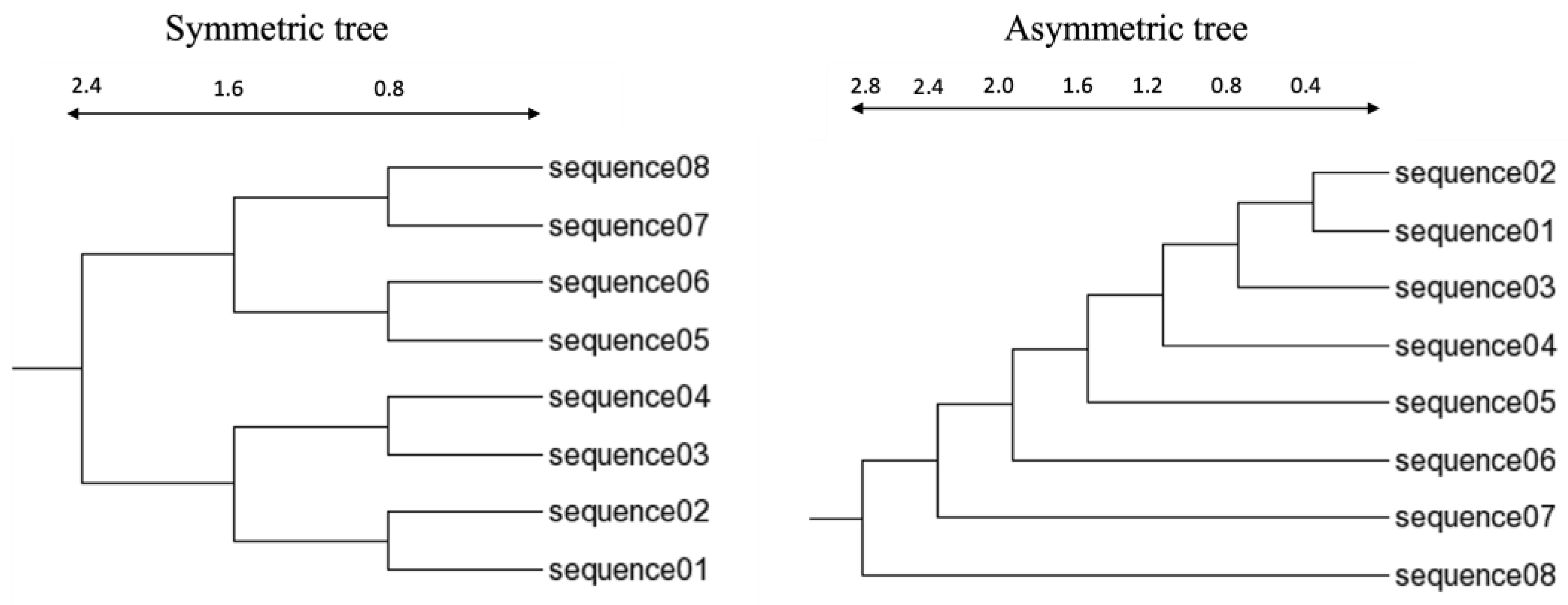
We generated our amino acid sequence datasets based on symmetric and asymmetric trees with 16 taxa (Figure 1) and 8 taxa (Figure 2). For the 16-taxa tree, two different sets of branch lengths were used to generate sequences with different levels of divergency, and 50 datasets have been generated for each tree. We used the Alisim tool, provided by IQ-TREE [34], to produce aligned sequences with an average length of 500 for each tree. The Jones–Taylor–Thornton (JTT) substitution model [35] was used for all datasets. There are two types of amino acid substitution models. The first type is based on counting empirical substitutions from a large number of aligned protein sequences, with the hope that the resulting substitution model will be one-hat-fits-all. The second type is derived from the maximum likelihood method based on a specific set of protein sequences (e.g., vertebrate mitochondrial proteins). They all specify the transition probabilities between amino acids given a branch length in a tree.
An insertion/deletion rate of 0.05 was used for both the 16-taxa and 8-taxa trees. The power law distribution (POW) was used as the insertion/deletion size, with a = 2 and power = 100. Therefore, we have the following four datasets based on 16-taxa trees: (1) a symmetric tree and (2) a half-symmetric tree, with branch lengths specified on the left panel of Figure 1, and and (3) an asymmetric tree and (4) a half-asymmetric tree, with branch lengths specified in the right panel of Figure 1. We have the following two datasets based on 8-taxa trees: (1) a symmetric tree and (2) an asymmetric tree with branch lengths specified in Figure 2. The simulated data and C source code implementing the 3-way alignment are included in the Supplementary Materials.

2.4. Measuring Distance Matrix and Constructing Guide Tree

For each dataset, we aligned all possible triplets (56 and 560 triplets for 8-taxa and 16-taxa topologies, respectively) using the Carrillo–Lipman algorithm with the BLOSUM62 matrix, a gap-open penalty of 10, and a gap-extension penalty of 2. Each pair of sequences exists in n 2 triplets. Therefore, to measure the distance between two sequences, we calculated the average over their distances in all those n 2 triplets. The final distance matrix contains the average distance of each sequence pair. We used the JTT model to measure evolutionary distances between each pair of sequences in the aligned triplets. The resulting distance matrices were then used as inputs to the NJ algorithm in the PHYLIP package to construct guide trees that would later be used in progressive multiple alignment.

2.5. Seqeuence Alignment with MAFFT

We compared the performance of MAFFT with the MAFFT-generated guide trees against the 3-way alignment guide trees. In this study, we assess the performance of three different algorithms of MAFFT, including FFT-NS-1, FFT-NS-2, and L-INS-i (which is the most accurate option in MAFFT). We used MAFFT default, except for specifying FFT-NS-1, FFT-NS-2, or L-INS-i. The FFT-NS-1 option measures distances based on the sharing of k-tuples between sequences (where k is typically 6). A guide tree is then reconstructed using UPGMA to guide the subsequent multiple alignment. FFT-NS-2 reconstructs a new guide tree using the alignment generated by FFT-NS-1 and realigns sequences based on the new tree. We expect FFT-NS-2 to generate a more accurate alignment compared to the FFT-NS-1 because of the recomputing of the guide tree. L-INS-i uses local alignments with the Smith–Waterman algorithm to generate a distance matrix instead of the k-tuple method. Moreover, it uses a new objective function combining the weighted sum-of-pair score (WSP) and COFFEE-like score, which measure the consistency between MSA and PSA [12].

2.6. Comparing the Accuracy of Phylogenetic Trees

MSAs generated in the previous step were used to construct phylogenetic trees using PhyML [36], with the option of simultaneously optimizing tree topology, branch length, and rates. These PhyML trees were then compared with the true tree for both the 16-taxa and 8-taxa trees, shown in Figure 1 and Figure 2, through calculation of Robinson–Foulds distances (RFds) [37]. The RFd between the true tree and the reconstructed tree is taken as a proxy for phylogenetic accuracy, where RFd = 0 means that the two trees share the same topology, and larger RFd values are associated with inaccuracies. RFd values between trees were computed using the APE package [38] in R. Note that RFd only measures the topological difference between trees but not the differences in branch lengths. Thus, a reconstructed tree would be considered identical to the true tree when RFd = 0, even if the two trees differ in branch lengths.

3. Results

3.1. Three-Way Alignment Tends to Generate Guide Trees Closer to the True Tree than Other Approaches

We first evaluated the two guide trees, one generated from the MAFFT L-INS-i option and the other using our three-way alignment (3-WAY in Table 1) by comparing them with the true tree (i.e., the tree used for sequence simulation). With the symmetric tree, both approaches recovered some true trees, but the three-way alignment approach recovered slightly more true trees (Table 1). Similarly, the RFd is greater for L-NS-i than it is for the three-way alignment approach. These results are consistent with our hypothesis that the three-way alignment approach would produce better guide trees. However, these differences are small and not statistically significant, given our sample size of 50 sets of simulated sequences (two-tailed paired-sample t-test, t = 1.1881, DF = 49 and p = 0.2405, Table 1). Given the effect size, a sample of 140 would be needed get a p value below 0.05.
With the asymmetric tree, neither the L-NS-i approach nor the three-way alignment results in a guide tree that is identical to the true tree (Table 1). However, the difference in the RFd, similar to the results with symmetric trees, is in the expected direction, i.e., being smaller for the three-way alignment than for the L-INS-i approach. However, the difference between the two groups is not statistically significant given the sample size of 50 for each group (t = 1.1586, DF = 49, p = 0.2522).
Table 2 presents the result of the comparisons of guide trees for 16-taxa trees. There are four different 16-taxa trees, including half-symmetric, symmetric, half-asymmetric, and asymmetric trees, which are represented as H-S tree, S tree, H-AS tree and AS tree, respectively, in Table 2. We compared the guide trees from four different approaches, including three-way alignment (3-WAY in Table 2) and the three MAFFT options (FFT-NS-1, FFT-NS-2, and L-INS-i), based on the simulated sequences. The guide trees reconstructed from k-tuple similarities (FFT-NS-1 and FFT-NS-2, with k = 6) are apparently much worse than those reconstructed from pairwise alignment (L-INS-i) or three-way alignment (Table 2). However, just as in Table 1, there is no significant difference between the last two approaches. The L-INS-i approach actually performed slightly better than the three-way alignment approach with the H-AS tree, recovering more true trees (41 versus 39) and having a smaller mean RFd (0.36 versus 0.52) than the three-way alignment approach (Table 2), although the difference is not statistically significant. The only difference reaching borderline significance involves the asymmetric tree (Table 2). The three-way alignment appears to produce a better guide tree, with an RFd nearly significantly smaller than that of the L-INS-i option (paired sample t-test, t = 1.8448, DF = 49, p = 0.0711).

3.2. Three-Way Alignment Leads to More Accurate Phylogenetic Results than Other Approaches

How will the difference in the guide tree affect the final phylogenetic reconstruction? We obtained MSA from each of the three types of guide trees as follows: (1) the true tree used for sequence simulation, (2) the guide tree reconstructed by the L-INS-i approach, and (3) the guide tree from the three-way alignment (3-WAY in Table 3). These MSAs are then used to reconstruct phylogenies by PhyML. We expect the MSAs obtained with the true tree as the guide tree to recover true trees but are interested in whether the three-way alignment approach will outperform the L-INS-i approach.
Using the true tree as the guide tree apparently increases the chance of the true tree being recovered through the aligned sequences, which is true for both the 8-taxa symmetric and asymmetric trees (Table 3). With the symmetric tree, the three-way alignment approach outperformed the L-NS-i approach, recovering more true trees and having a smaller mean RFd (Table 3). However, the difference is not statistically significant given the sample size of 50 for each group (two-tailed paired-sample t-test, t = 1.4289, DF = 49, p = 0.1594).
With the asymmetric tree, none of the 50 MSAs from the L-INS-i approach recovered a true tree, and neither did the three-way alignment approach (Table 3). However, the RFd is smaller for the three-way alignment approach (mean RFd = 5) than that of the L-NS-i approach (RFd = 6). The difference is statistically significant based on a paired-sample t-test (t = 3.6293, DF = 49, p = 0.0007). This difference between the L-INS-i and the three-way alignment approach is also consistent with the results in Table 1.
We also performed the same comparison of phylogenetic results from the 16-taxa trees (Table 4). We compared the accuracy of the reconstructed phylogenetic trees from the FFT-NS-1, FFT-NS-2, L-INS-i, and three-way alignment methods. The results are similar to those in Table 2, i.e., the guide trees reconstructed from six-tuple similarities (FFT-NS-1 and FFT-NS-2) are worse than those reconstructed from pairwise alignment (L-INS-i) or three-way alignment (Table 4). When the true tree was used as the guide tree, the resulting MSA recovered the true tree, except in the case of the asymmetric tree (AS tree in Table 4). Thus, the true tree is indeed the best guide tree, although there are controversies on this seemingly self-evident statement, as we will discuss later.
For the half-symmetric tree (H-S tree) and half-asymmetric tree (H-AS tree), because of reduced sequence divergence, the true tree was recovered from most of the datasets. Even the FFT-NS-1 and the FFT-NS-2 approaches perform well, recovering 90% and 94% of the true trees, respectively, in the H-S tree case and 80% and 81% in the H-AS case (Table 4).
For the symmetric tree (S tree in Table 4), the FFT-NS-1 and FFT-NS-2 approaches recovered few true trees, but the L-INS-i and the three-way approaches recovered most of the true trees (Table 4). RFd is slightly smaller for the three-way alignment approach than it is for the L-INS-i approach, but the difference is not significant (paired-sample t-test, t = 0.7035, DF = 49, p = 0.2425). For the asymmetric tree (AS tree in Table 4), both the L-INS-i and the three-way alignment approaches recovered few true trees. The RFd is slightly smaller for the three-way alignment approach, but the difference is not significant (paired-sample t-test, t = 0.4928, DF = 49, p = 0.6244).

3.3. Accuracy of the Guide Tree Affects the Accuracy of the Final Tree from MSA

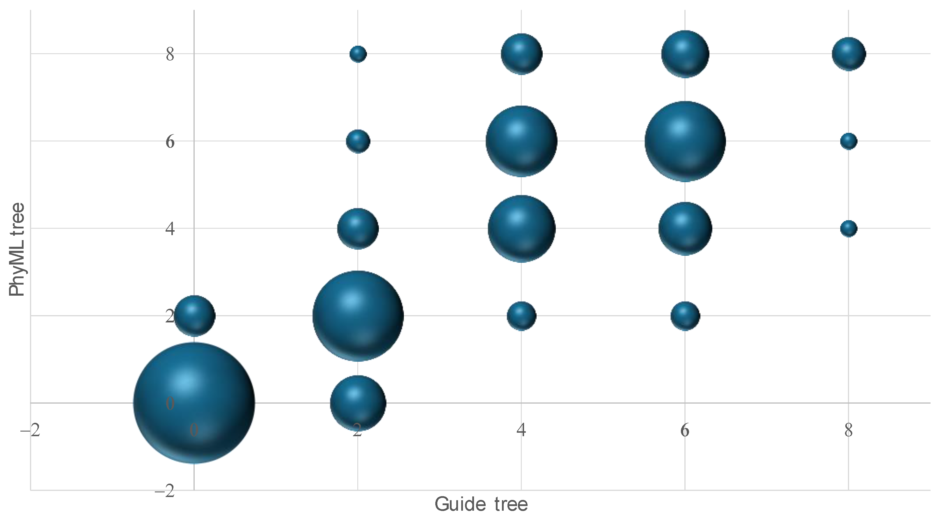
We evaluated the hypothesis that the quality of guide trees directly influences the phylogenetic accuracy by directly examining the association in RFd between the guide tree and the final phylogenetic reconstruction from PhyML. For the 8-taxa tree, we combined results from two simulations (symmetric and asymmetric trees) and the two types of guide trees (the L-INS-i and three-way alignment approaches), so that there are 200 guide trees and 200 PhyML trees from the resulting MSA. There is a strong association in RFd between the guide tree and the PhyML-reconstructed final tree (Figure 3). When the guide tree has an identical topology as the true tree (RFd = 0 between the two), the resulting PhyML-reconstructed tree also tend to have the topology of the true tree; when the guide tree deviates much from the true tree, so does the resulting PhyML-reconstructed tree (Figure 3).
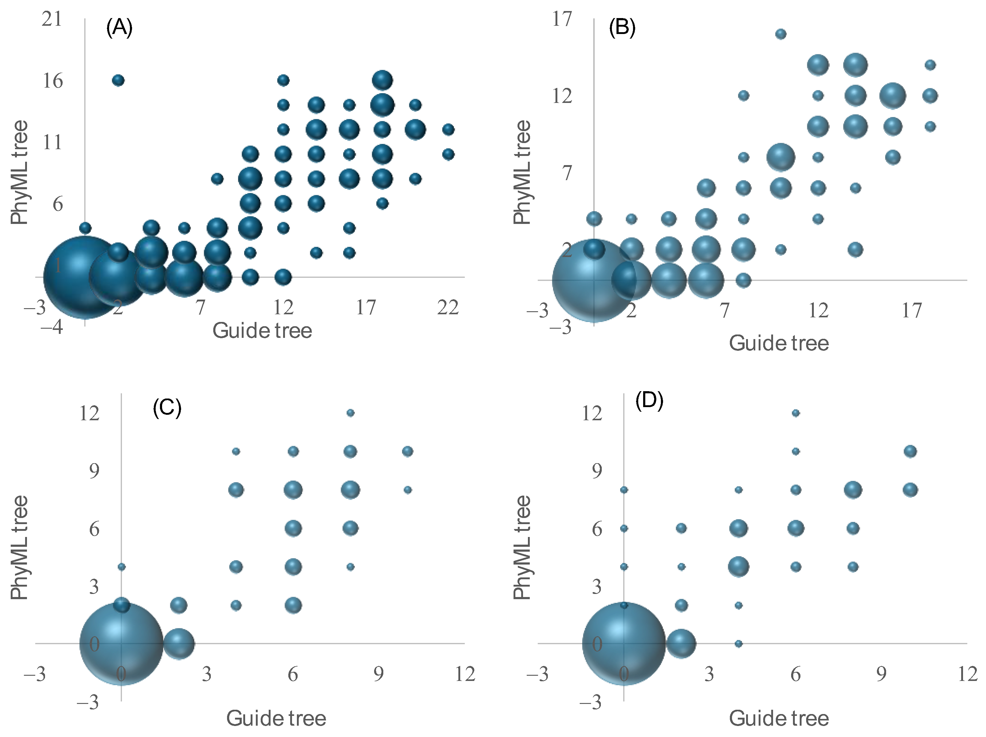
We have done the same for 16-taxa trees (Figure 4), including the fast but inaccurate FFT-NS-1 and FFT-NS-2 options in MAFFT, in addition to the L-INS-i and three-way alignment approaches. For each of these approaches, we combined the results from four simulations (the symmetric and asymmetric trees and the half-symmetric and half-asymmetric trees). Thus, each sub-figure in Figure 4 includes 200 guide trees and 200 PhyML trees. It is clear that the two fast and inaccurate options (that generate guide trees from six-tuple similarities) produced poor guide trees (large RFd values), as well as the final PhyML trees from the resulting MSA (Figure 4A,B) relative to the L-INS-i approach that generated the guide tree from local pairwise alignment (Figure 4C) or to the three-way alignment approach (Figure 4D). However, for all the four approaches, the guide tree quality strongly affects the accuracy of the final PhyML tree (Figure 4). The relationship between the guide tree RFd and PhyML tree RFd are all highly significant (p < 0.0001).

3.4. Sum-of-Pair Score May Not Be a Good Criterion for Choosing the Best MSA

There are two criteria that can be used to evaluate the quality of an MSA. The first is phylogenetic accuracy, i.e., the MSA that results in the most accurate phylogenetic reconstruction is the best MSA. This criterion is conceptually fine but not computationally practical. Also, one can generally evaluate phylogenetic accuracy only for simulated sequences with a known true tree. The second criterion is the sum-of-pair score (SPS) or its variations, such as weighted SPS [39,40,41]. This weighted SPS is used in the default option in MUSCLE and the G-INS-i and L-INS-i options in MAFFT. The criterion is computationally practical and expected to be generally consistent with the first criterion. Our results in the previous section show that when an MSA is generated with the true tree as a guide tree, this MSA tends to result in the most accurate phylogenetic reconstruction. It is, therefore, interesting to know if an MSA generated with the true tree as a guide tree also leads to the highest SPS.
We compared SPS from two types of MSAs, one generated using the true tree as the guide tree (the “trueTree” approach) and the other generated using the accurate L-INS-i option (the “L-INS-i” approach, which creates the guide tree based on local pairwise alignment) in MAFFT. The input sequences are simulated with symmetric and asymmetric trees as before, with an average sequence length of 500 amino acids. Each simulated data set generated two MSAs, one from the trueTree approach and the other from the L-INS-i approach. The two MSAs were also used for phylogenetic reconstruction using PhyML. When the true tree was used as a guide tree, the final PhyML tree was closer to the true tree (smaller RFd) than that of the L-INS-i approach (Figure 5A,C). This difference is highly significant based on a paired-sample t-test (p < 0.0001 for data in Figure 5A,C). Thus, when phylogenetic accuracy is used as a criterion, the MSA resulting from using the true tree as a guide tree is better than MSA from the L-INS-i approach.
Surprisingly, SPS is higher for the MSA from the L-INS-i than the MSA from using the true tree as the guide tree (Figure 5B,C). This is consistent for both the asymmetric tree and the symmetric tree. The difference is highly significant based on a paired-sample t-test (p < 0.0001). This creates a conflict in choosing the best MSA. With the criterion of phylogenetic accuracy as a criterion, the MSA from the trueTree approach is better; with the SPS as the criterion, the MSA from the L-INS-i approach is better.
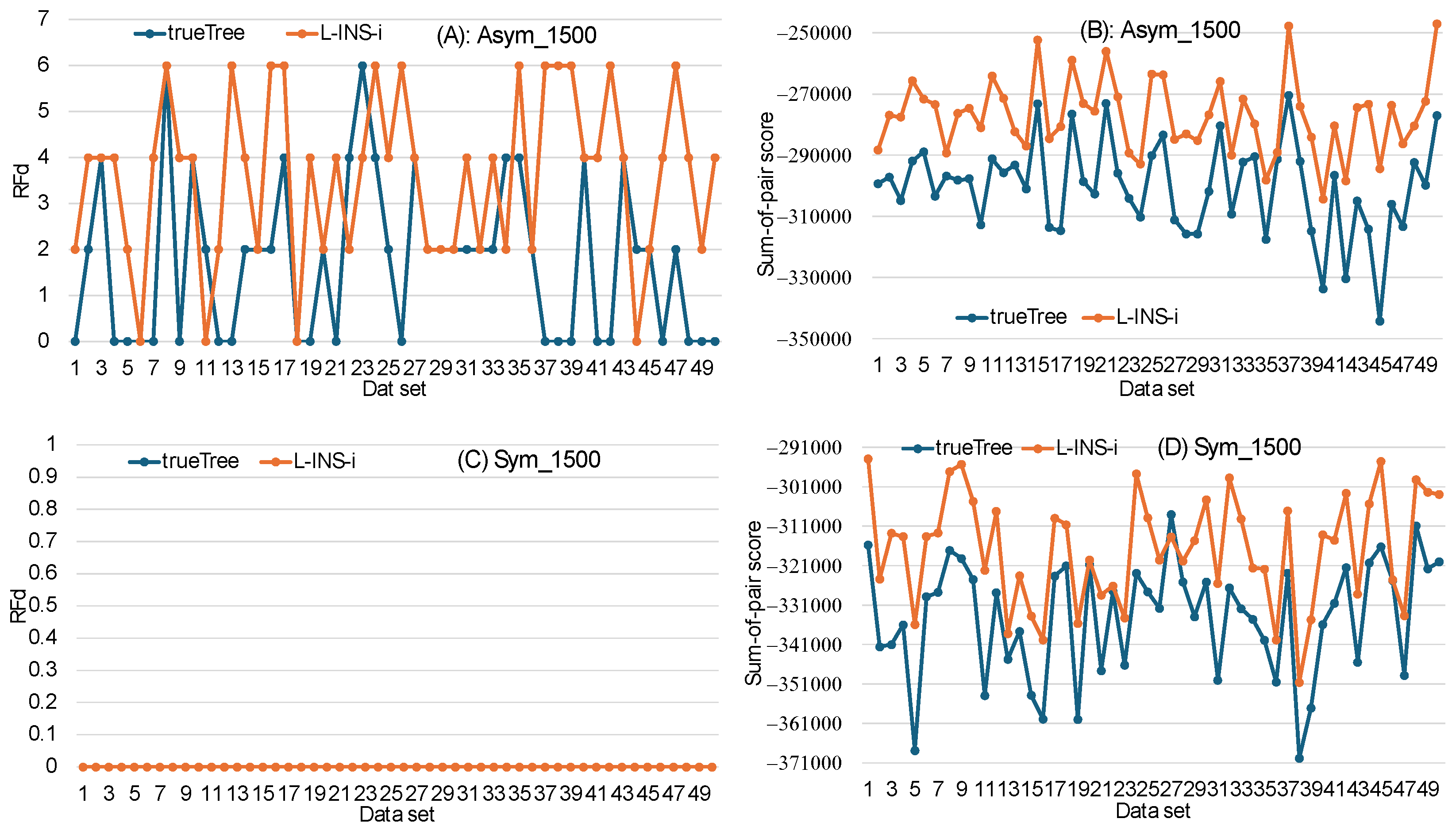
To further confirm the results in Figure 5, we simulated longer sequences with an average length of 1500 amino acids according to those symmetric and asymmetric trees. The same computation was repeated. For asymmetric trees (Figure 6A), the trueTree approach (MSA obtained with the true tree as a guide tree) generated PhyML trees more similar than those generated from the L-INS-i approach. This difference in RFd between the trueTree and the L-INS-i approaches is highly significant (paired-sample t-test, p < 0.0001). The longer sequence length allowed both the trueTree and the L-INS-i approaches to recover all symmetric true trees (Figure 6C). Thus, the criterion of phylogenetic accuracy still favors the trueTree approach over the L-INS-i approach. The relevant scatter plots for dataset used in Figure 5 and Figure 6 are provided in Supplementary Materials.
In contrast, SPS is higher for MSA from the L-INS-i approach than that of the trueTree approach (Figure 6B,C), which is consistent with the results in Figure 5. Thus, the SPS criterion tends to favor MSAs that do not generate the best tree. The conflict between the two criteria appears real.

3.5. Performance of the Three-Way Alignment on Benchmark Datasets

We performed a quick evaluation of the performance of the three-way alignment approach by using the BAliBASE [42] benchmark datasets of protein sequences. We selected 60 highly diverged reference alignments, including (1) the first 20 sets in in RV11 (BB110001-BB11020), (2) 20 randomly chosen sets in RV30, and (3) 20 arbitrarily chosen sets from RV12 (BB12002-BB12006, BB12009, BB12010, BB12012-BB12024). These MSAs were corroborated with other information, such as protein structure, and may be considered the best approximation of the true alignment. From each of these 60 sets of protein sequences, we generated two additional alignments, one from MAFFT with the accurate L-INS-i option and the other from the three-way alignment approach. These three MSAs are referred to as BAliBase, L-INS-i, and three-way. From each alignment, a PhyML tree is built with the default LG model and the simultaneous optimization of tree topology, branch lengths, and rates. The three resulting trees were also designated BAliBase, L-INS-i, and three-way, respectively. The BAliBase tree was taken as the best approximation of the true tree. The RFd value was calculated between the BAliBase tree and the L-INS-i tree and between the BAliBase tree and the thee-way tree. The results are similar to those with simulated sequences. The mean RFd is 3.03333 between the BAliBase and L-INS-i trees and 2.66667 between the BAliBase and three-way trees. The two are marginally significant based on a one-tailed paired-sample test (t = 1.6638, DF = 59, one-tailed p = 0.0507).

4. Discussion

There are disagreements involving guide trees in progressive multiple sequence alignment. First, what is the best guide tree for progressive multiple sequence alignment? Second, how can we obtain the best guide tree? There are also disagreements on what criterion should be used in choosing the optimal MSA. If phylogenetic reconstruction is the ultimate goal, then phylogenetic accuracy obviously should be the ultimate criterion for choosing the best MSA. Given that this criterion cannot be practically used, does the SPS criterion serve as a good proxy? This study aims to address these questions, with a focus on highly diverged sequences that are hard to align.

4.1. Is the True Tree the Best Guide Tree for Progressive Multiple Sequence Alignment?

One would tend to assume that the true tree should be the best guide tree. However, this assumption conflicts with the principle that multiple sequence alignment should start with the most similar sequences and progress toward less similar sequences (R. C. Edgar, pers. comm.). This conflict is illustrated with the following true tree:
((S1:0.001, S2:0.1):0.001, (S3:0.001,S4:0.1):0.001).
S1 and S3 are the most similar sequences, with a pairwise distance of only 0.003. They should therefore be aligned first following the principle stated above. However, the true tree would not allow S1 and S3 to be aligned first and would force S1 and S2 (or S3 and S4) to be aligned first. This is one of the reasons for widely used multiple sequence alignment programs, such as MAFFT [12] and MUSCLE [13], to use a modified version of UPGMA to reconstruct the guide tree, because UPGMA will cluster S1 and S3 together. Such a guide tree ensures that S1 and S3 would be aligned first. Will such a guide tree and the resulting MSA cause phylogenetic distortion in the final reconstructed tree? Our results, especially those in Table 3 and Figure 3 and Figure 4, suggest that if the accuracy of the final phylogeny is taken as a criterion, the true tree indeed is the best guide tree. Version 5 of MUSCLE [43] includes an ensemble of trees for exploring the consequence of the resulting MSA on phylogenetic reconstruction. This would help phylogeneticists appreciate the variation in guide trees and the resulting reconstructed phylogenies.

4.2. How to Obtain the Best Guide Tree?

If we agree that the true tree is the best guide tree, then how do we obtain a guide that is the best approximation of this true tree? In this research, we explore the potential of three-way alignment in improving the accuracy of the guide tree. Our results are consistent with the hypothesis that three-way alignment can produce better guide trees (exhibiting lower RFd with true tree) compared to guide trees from PSA or k-tuple approaches, leading to improved MSAs and the phylogenetic reconstruction based on the MSAs (Table 1, Table 2, Table 3 and Table 4). Two lines of evidence were presented to support the conclusion that the guide tree from the three-way alignment (3-WAY) is better than that generated from the most accurate option in MAFFT (L-INS-i, which creates the initial guide tree from local pairwise alignment). First, the guide tree from the 3-WAY approach is closer to the true tree than that from the L-INS-i approach. Second, when the MSA generated from 3-WAY and L-INS-i guide trees were fed to PhyML for phylogenetic reconstruction, the MSA from the 3-WAY guide tree produced PhyML trees closer to the true tree than that from the L-INS-i approach.
While guide trees based on k-tuple similarities in MAFFT are poor, the guide tree from the L-INS-i option in MAFFT is very good, and three-way alignment may be useful only in the most challenging cases with extremely diverged sequences. Sequences simulated from our half-symmetric and half-asymmetric trees are comparable in divergence to many real homologous amino acid sequences, yet MAFFT performed well with these sequences. Only with the highly diverged sequences simulated from the asymmetric trees did MAFFT experience difficulties in generating quality MSA (Table 1, Table 2, Table 3 and Table 4).

4.3. Is Sum-of-Pair Score or Its Derivative a Good Criterion for Choosing the Best MSA?

The best MSA should produce the true tree, especially when the objective of sequence alignment is accurate phylogenetic reconstruction. However, phylogenetic accuracy cannot be used directly as a criterion because the true tree is unknown, except in simulated sequences. One would hope that the sum-of-pair score (SPS) or its variations, such as weighted SPS, which is computationally practical and widely used as a criterion for choosing the best MSA, would be equivalent to the criterion of phylogenetic accuracy. In other words, the MSA with the highest SPS is also the MSA that would result in the most accurate phylogeny. Our results (Figure 5 and Figure 6) suggest that this is not the case. From each set of our simulated sequences, two MSAs were produced, one with the true tree as the guide tree (trueTree) and the other using the guide tree from the L-INS-i approach (L-INS-i). When these two MSAs were fed to PhyML for phylogenetic reconstruction, the MSA from the trueTree approach produced trees more similar to the true tree than that from the L-INS-i approach. However, the latter has significantly higher SPS than the former. Thus, the two criteria are inconsistent.
It is difficult to provide a specification of time complexity with the Carrillo–Lipman algorithm. This algorithm for the three-way alignment includes three pair-wise alignments, followed by a simplified three-way alignment that does not need to visit all cells in the cube. The time complexity for this last step is difficult to express because the time required for this step depends on the nature of the three sequences. If the three sequences are nearly identical, then we have the best scenario, and the time required for this step would be almost linear. If the three sequences are highly diverged and differ much in length (i.e., many indel events), then the time requirement for this step would be similar to the plain three-way alignment using dynamic programming. Because we aim to improve the sequence alignment of highly diverged sequences, the time saved with the Carrillo–Lipman algorithm is not substantial.
One time-saving protocol is to first identify regions of consistency among the three pairwise alignments in each three-way alignment using the approach proposed by Gotoh [44]. The regions of consistency do not need three-way alignment. They can serve as anchors so that one only needs to do three-way alignment for sequence segments between such anchors.

5. Conclusions

In progressive multiple sequence alignment, the quality of a guide tree affects the quality of MSA and the quality of subsequent phylogenetic reconstruction. The three-way alignment improves the quality of the guide trees and results in more accurate phylogenetic reconstruction. The two criteria for choosing the best MSA, phylogenetic accuracy and sum-of-pair score, conflict with each other.

Supplementary Materials

The following supporting information can be downloaded at: https://www.mdpi.com/article/10.3390/a17050205/s1, simulated data in directories 8tax_dataset, 16taxa_dataset, MSA_length1500; source code in directory Source_code. Equivalent scatter plots for Figure 5 and Figure 6 in SuppfileS1.xlsx.

Author Contributions

M.A.R. and X.X. designed the study. M.A.R. developed the algorithm, designed and wrote the relevant software, simulated, and analyzed the data. M.A.R. wrote the original draft of the manuscript. M.A.R., A.K. and X.X. reviewed and edited the manuscript. X.X. supervised and coordinated the study. All authors have read and agreed to the published version of the manuscript.

Funding

This work is supported by the Natural Sciences and Engineering Research Council of Canada (NSERC) Discovery Grant to X.X. [RGPIN-2024-05641].

Institutional Review Board Statement

Not applicable.

Informed Consent Statement

Not applicable.

Data Availability Statement

Data are contained within the article and in the Supplementary Materials.

Acknowledgments

We would like to thank Kazutaka Katoh for detailed explanations on MAFFT and Robert C. Edgar for the discussion on why the true tree may not necessarily be a good guide tree for sequence alignment. Stephane Aris-Brosou, Arvind Mer, and Marcel Turcotte provided many comments that improved the manuscript. The computational resources were provided by Compute Canada. Three anonymous reviews and editorial feedback improved the manuscript substantially.

Conflicts of Interest

The authors declare that there are no conflicts of interest.

References

  1. Xia, X. Post-Alignment Adjustment and Its Automation. Genes 2021, 12, 1809. [Google Scholar] [CrossRef] [PubMed]
  2. Hall, B.G. Comparison of the Accuracies of Several Phylogenetic Methods Using Protein and DNA Sequences. Mol. Biol. Evol. 2005, 22, 792–802. [Google Scholar] [CrossRef] [PubMed]
  3. Goldman, N. Effects of Sequence Alignment Procedures on Estimates of Phylogeny. BioEssays 1998, 20, 287–290. [Google Scholar] [CrossRef]
  4. Morrison, D.A.; Ellis, J.T. Effects of Nucleotide Sequence Alignment on Phylogeny Estimation: A Case Study of 18S rDNAs of Apicomplexa. Mol. Biol. Evol. 1997, 14, 428–441. [Google Scholar] [CrossRef] [PubMed]
  5. Needleman, S.B.; Wunsch, C.D. A General Method Applicable to the Search for Similarities in the Amino Acid Sequence of Two Proteins. J. Mol. Biol. 1970, 48, 443–453. [Google Scholar] [CrossRef] [PubMed]
  6. Eddy, S.R. What Is Dynamic Programming? Nat. Biotechnol. 2004, 22, 909–910. [Google Scholar] [CrossRef] [PubMed]
  7. Sankoff, D. Minimal Mutation Trees of Sequences. SIAM J. Appl. Math. 1975, 28, 35–42. [Google Scholar] [CrossRef]
  8. Sankoff, D.; Cedergren, R.J.; Lapalme, G. Frequency of Insertion-Deletion, Transversion, and Transition in the Evolution of 5S Ribosomal RNA. J. Mol. Evol. 1976, 7, 133–149. [Google Scholar] [CrossRef] [PubMed]
  9. Hirschberg, D.S. A Linear Space Algorithm for Computing Maximal Common Subsequences. Commun. ACM 1975, 18, 341–343. [Google Scholar] [CrossRef]
  10. Smith, T.F.; Waterman, M.S. Identification of Common Molecular Subsequences. J. Mol. Biol. 1981, 147, 195–197. [Google Scholar] [CrossRef]
  11. Feng, D.-F.; Doolittle, R.F. Progressive Sequence Alignment as a Prerequisite to Correct Phylogenetic Trees. J. Mol. Evol. 1987, 25, 351–360. [Google Scholar] [CrossRef] [PubMed]
  12. Katoh, K.; Misawa, K.; Kuma, K.; Miyata, T. MAFFT: A Novel Method for Rapid Multiple Sequence Alignment Based on Fast Fourier Transform. Nucleic Acids Res. 2002, 30, 3059–3066. [Google Scholar] [CrossRef] [PubMed]
  13. Edgar, R.C. MUSCLE: Multiple Sequence Alignment with High Accuracy and High Throughput. Nucleic Acids Res. 2004, 32, 1792–1797. [Google Scholar] [CrossRef] [PubMed]
  14. Notredame, C.; Higgins, D.G.; Heringa, J. T-Coffee: A Novel Method for Fast and Accurate Multiple Sequence alignment11Edited by J. Thornton. J. Mol. Biol. 2000, 302, 205–217. [Google Scholar] [CrossRef] [PubMed]
  15. Thompson, J.D.; Higgins, D.G.; Gibson, T.J. CLUSTAL W: Improving the Sensitivity of Progressive Multiple Sequence Alignment through Sequence Weighting, Position-Specific Gap Penalties and Weight Matrix Choice. Nucleic Acids Res. 1994, 22, 4673–4680. [Google Scholar] [CrossRef] [PubMed]
  16. Thompson, J.D.; Plewniak, F.; Poch, O. A Comprehensive Comparison of Multiple Sequence Alignment Programs. Nucleic Acids Res. 1999, 27, 2682–2690. [Google Scholar] [CrossRef] [PubMed]
  17. Noah, K.E.; Hao, J.; Li, L.; Sun, X.; Foley, B.; Yang, Q.; Xia, X. Major Revisions in Arthropod Phylogeny through Improved Supermatrix, with Support for Two Possible Waves of Land Invasion by Chelicerates. Evol. Bioinform. Online 2020, 16, 1176934320903735. [Google Scholar] [CrossRef]
  18. Regier, J.C.; Shultz, J.W.; Zwick, A.; Hussey, A.; Ball, B.; Wetzer, R.; Martin, J.W.; Cunningham, C.W. Arthropod Relationships Revealed by Phylogenomic Analysis of Nuclear Protein-Coding Sequences. Nature 2010, 463, 1079–1083. [Google Scholar] [CrossRef] [PubMed]
  19. Xia, X. PhyPA: Phylogenetic Method with Pairwise Sequence Alignment Outperforms Likelihood Methods in Phylogenetics Involving Highly Diverged Sequences. Mol. Phylogenetics Evol. 2016, 102, 331–343. [Google Scholar] [CrossRef]
  20. Bellamy-Royds, A.B.; Turcotte, M. Can Clustal-Style Progressive Pairwise Alignment of Multiple Sequences Be Used in RNA Secondary Structure Prediction? BMC Bioinform. 2007, 8, 190. [Google Scholar] [CrossRef]
  21. Masoumi, B.; Turcotte, M. Simultaneous Alignment and Structure Prediction of Three RNA Sequences. Int. J. Bioinform. Res. Appl. 2005, 1, 230–245. [Google Scholar] [CrossRef] [PubMed]
  22. Xia, X. Phylogenetic Relationship Among Horseshoe Crab Species: Effect of Substitution Models on Phylogenetic Analyses. Syst. Biol. 2000, 49, 87–100. [Google Scholar] [CrossRef] [PubMed]
  23. Xia, X.; Xie, Z.; Kjer, K.M. 18S Ribosomal RNA and Tetrapod Phylogeny. Syst. Biol. 2003, 52, 283–295. [Google Scholar] [CrossRef] [PubMed]
  24. Zhan, Q.; Ye, Y.; Lam, T.-W.; Yiu, S.-M.; Wang, Y.; Ting, H.-F. Improving Multiple Sequence Alignment by Using Better Guide Trees. BMC Bioinform. 2015, 16, S4. [Google Scholar] [CrossRef] [PubMed]
  25. Capella-Gutiérrez, S.; Gabaldón, T. Measuring Guide-Tree Dependency of Inferred Gaps in Progressive Aligners. Bioinformatics 2013, 29, 1011–1017. [Google Scholar] [CrossRef] [PubMed]
  26. Penn, O.; Privman, E.; Landan, G.; Graur, D.; Pupko, T. An Alignment Confidence Score Capturing Robustness to Guide Tree Uncertainty. Mol. Biol. Evol. 2010, 27, 1759–1767. [Google Scholar] [CrossRef] [PubMed]
  27. Nelesen, S.; Liu, K.; Zhao, D.; Linder, C.R.; Warnow, T. The Effect of the Guide Tree on Multiple Sequence Alignments and Subsequent Phylogenetic Analyses. In Biocomputing 2008; World Scientific: Singapore, 2007; pp. 25–36. ISBN 978-981-277-608-2. [Google Scholar]
  28. Ye, Y.; Cheung, D.W.; Wang, Y.; Yiu, S.-M.; Zhan, Q.; Lam, T.-W.; Ting, H.-F. GLProbs: Aligning Multiple Sequences Adaptively. In Proceedings of the International Conference on Bioinformatics, Computational Biology and Biomedical Informatics, Wshington, DC, USA, 22–25 September 2013; Association for Computing Machinery: New York, NY, USA; pp. 152–160. [Google Scholar]
  29. Kruspe, M.; Stadler, P.F. Progressive Multiple Sequence Alignments from Triplets. BMC Bioinform. 2007, 8, 254. [Google Scholar] [CrossRef] [PubMed]
  30. Chien, R.-T.; Liao, Y.-L.; Wang, C.-A.; Li, Y.-C.; Lu, Y.-C. Three-Dimensional Dynamic Programming Accelerator for Multiple Sequence Alignment. In Proceedings of the 2018 IEEE Nordic Circuits and Systems Conference (NORCAS): NORCHIP and International Symposium of System-on-Chip (SoC), Tallinn, Estonia, 30–31 October 2018; pp. 1–5. [Google Scholar]
  31. Gotoh, O. Alignment of Three Biological Sequences with an Efficient Traceback Procedure. J. Theor. Biol. 1986, 121, 327–337. [Google Scholar] [CrossRef] [PubMed]
  32. Carrillo, H.; Lipman, D. The Multiple Sequence Alignment Problem in Biology. SIAM J. Appl. Math. 1988, 48, 1073–1082. [Google Scholar] [CrossRef]
  33. Huang, X. Alignment of Three Sequences in Quadratic Space. SIGAPP Appl. Comput. Rev. 1993, 1, 7–11. [Google Scholar] [CrossRef]
  34. Ly-Trong, N.; Naser-Khdour, S.; Lanfear, R.; Minh, B.Q. AliSim: A Fast and Versatile Phylogenetic Sequence Simulator for the Genomic Era. Mol. Biol. Evol. 2022, 39, msac092. [Google Scholar] [CrossRef] [PubMed]
  35. Jones, D.T.; Taylor, W.R.; Thornton, J.M. The Rapid Generation of Mutation Data Matrices from Protein Sequences. Bioinformatics 1992, 8, 275–282. [Google Scholar] [CrossRef]
  36. Guindon, S.; Dufayard, J.-F.; Lefort, V.; Anisimova, M.; Hordijk, W.; Gascuel, O. New Algorithms and Methods to Estimate Maximum-Likelihood Phylogenies: Assessing the Performance of PhyML 3.0. Syst. Biol. 2010, 59, 307–321. [Google Scholar] [CrossRef]
  37. Robinson, D.F.; Foulds, L.R. Comparison of Phylogenetic Trees. Math. Biosci. 1981, 53, 131–147. [Google Scholar] [CrossRef]
  38. Paradis, E.; Claude, J.; Strimmer, K. APE: Analyses of Phylogenetics and Evolution in R Language. Bioinformatics 2004, 20, 289–290. [Google Scholar] [CrossRef] [PubMed]
  39. Edgar, R.C.; Batzoglou, S. Multiple Sequence Alignment. Curr. Opin. Struct. Biol. 2006, 16, 368–373. [Google Scholar] [CrossRef]
  40. Gotoh, O. A Weighting System and Aigorithm for Aligning Many Phylogenetically Related Sequences. Bioinformatics 1995, 11, 543–551. [Google Scholar] [CrossRef]
  41. Altschul, S.F.; Carroll, R.J.; Lipman, D.J. Weights for Data Related by a Tree. J. Mol. Biol. 1989, 207, 647–653. [Google Scholar] [CrossRef] [PubMed]
  42. Thompson, J.D.; Koehl, P.; Ripp, R.; Poch, O. BAliBASE 3.0: Latest Developments of the Multiple Sequence Alignment Benchmark. Proteins Struct. Funct. Bioinform. 2005, 61, 127–136. [Google Scholar] [CrossRef]
  43. Edgar, R.C. Muscle5: High-Accuracy Alignment Ensembles Enable Unbiased Assessments of Sequence Homology and Phylogeny. Nat. Commun. 2022, 13, 6968. [Google Scholar] [CrossRef]
  44. Gotoh, O. Consistency of Optimal Sequence Alignments. Bull. Math. Biol. 1990, 52, 509–525. [Google Scholar] [CrossRef] [PubMed]
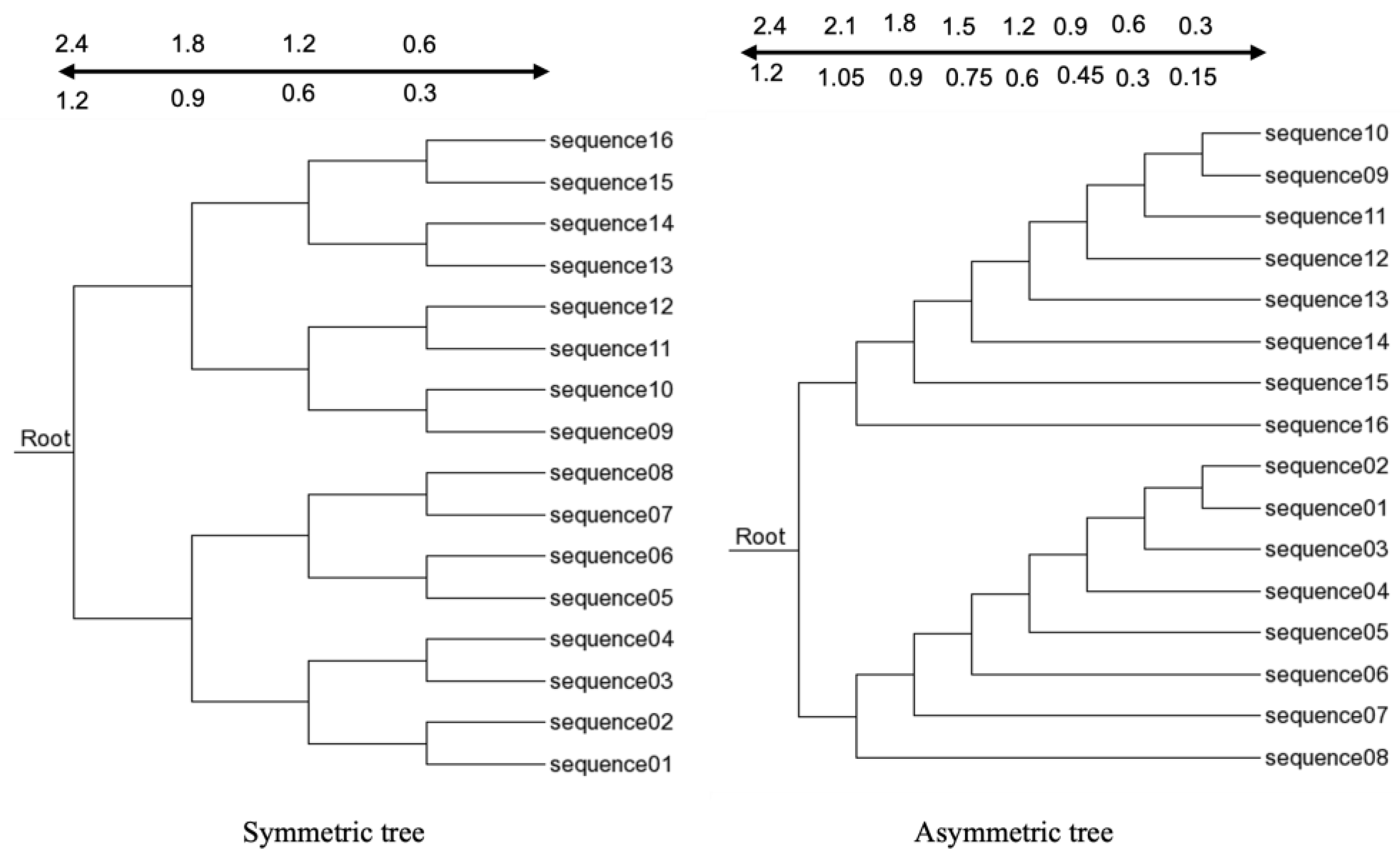
Figure 1. The 16-taxa trees used for simulating sequences. The branch lengths from the leaf to each internal node are indicated by the scale above the tree. Trees referred to as symmetric and asymmetric trees use the top numbers of the scale. Trees referred to as half-symmetric and half-asymmetric trees use the bottom numbers of the scale.
Algorithms 17 00205 g001
Figure 2. Eight-taxa trees used for simulating sequences of high divergence. The scale indicates the branch lengths from the leaf to the internal nodes.
Algorithms 17 00205 g002
Figure 3. Relationship between RFd of a guide tree and RFd of the corresponding PhyML tree from the resulting MSA, based on the 8-taxa symmetric and asymmetric trees. A bubble plot was used because many points overlap each other. The relationship is highly significant (n = 200, r = 0.83143, p < 0.0001).
Algorithms 17 00205 g003
Figure 4. Relationship between RFd of guide trees and RFd of phylogenetic trees generated by PhyML, based on 16-taxa trees. (A) FFT-NS-1 approach in which the guide tree was generated from 6-tuple similarities. (B) FFT-NS-2 approach in which the guide tree is recomputed from the first round of multiple sequence alignment. (C) L-INS-i approach in which the guide tree is from local pairwise alignment. (D) Three-way alignment approach in which the guide tree was described in the Section 2. A bubble plot was used because many points overlapped with each other.
Algorithms 17 00205 g004
Figure 5. Conflict between two criteria (phylogenetic accuracy and sum-of-pair score) in choosing the best MSA. Sequences with an average length of 500 are simulated with the 16-taxa symmetric and asymmetric trees. Two MSAs were produced from each set of sequences, one with the true tree as the guide tree (trueTree) and the other with the L-INS-i approach (L-INS-i), which generates a guide tree from local pairwise alignment. Sum-of-pair score was calculated for each MSA. PhyML was used for phylogenetic reconstruction for each MSA, and the Robinson–Foulds distance (RFd) was calculated between the true tree and the PhyML tree. The trueTree approach produced PhyML trees closer to the true tree than that of the L-INS-i approach for both the asymmetric tree (A) and symmetric tree (C). However, the L-INS-i approach produced MSAs with higher sum-of-pair scores than that of the trueTree approach, which is true for both the asymmetric tree (B) and symmetric tree (D).
Algorithms 17 00205 g005
Figure 6. Conflict between two criteria (phylogenetic accuracy and sum-of-pair score) in choosing the best MSA. Sequences with an average length of 1500 are simulated with the 16-taxa symmetric and asymmetric trees. Computations are the same as in Figure 5. The trueTree approach produced PhyML trees closer to the true tree than those of the L-INS-i approach for both the asymmetric trees (A), and both algorithms produced PhyML trees identical to true tree for the symmetric tree (C). However, the L-INS-i approach produced MSAs with higher sum-of-pair scores than those of the trueTree approach, which is true for both the asymmetric tree (B) and symmetric tree (D).
Algorithms 17 00205 g006
Table 1. Rresult of comparing guide trees generated uising 3-way alignment and L-INS-i methods based on simulated amino acid sequences on 8-taxa symmetric and asymmetric trees.
Symmetric TreeAsymmetric Tree
Guide TreeNtrue (1)RFd (2)SERFd (3)Ntrue (1)RFd (2)SERFd (3)
L-INS-i270.920.142405.120.1993
3-WAY310.760.138704.840.2067
(1) Ntrue: the number of correctly reconstructed trees (RFd = 0) using a method. (2) RFd: mean RFd from 50 simulated sets of sequences. (3) SERFd: standard error of RFd.
Table 2. Quality of guide trees generated using three MAFFT options (FFT-NS-1, FFT-NS-2, L-INS-i) and the 3-way alignment (3-WAY), based on simulated amino acid sequences the 16-taxa trees, including half-symmetric (H-S tree), symmetric (S tree), half-asymmetric (H-AS tree), and asymmetric (AS tree) trees. Other column labels are the same as in Table 1.
H-S TreeS TreeH-AS TreeAS Tree
Guide TreeNtrueRFdSERFdNtrueRFdSERFdNtrueRFdSERFdNtrueRFdSERFd
FFT-NS-1351.080.269309.240.5107152.520.3514015.320.5817
FFT-NS-2341.280.295607.240.4495291.160.24970130.4891
L-INS-i5000390.60.1429410.360.109806.480.2325
3-WAY5000400.40.1143390.520.149135.80.3886
Table 3. Phylogenetic accuracy from different guide trees. Sequences were simulated for the 8-taxa symmetric and asymmetric trees. MSAs were generated (1) with the true tree (True Tree), (2) from the L-INS-i option (L-INS-i), and (3) from the 3-way alignment (3-WAY). Phylogenetic reconstruction was performed with PhyML. Other column headings are the same as in Table 2.
Symmetric TreeAsymmetric Tree
Guide TreeNtrueRFdSERFdNtrueRFdSERFd
True Tree5000211.520.2180
L-INS-i290.920.1637060.2356
3-WAY340.680.1469050.2231
Table 4. Result of comparing the reconstructed phylogenetic trees using PhyML and MSA generated with FFT-NS-1, FFT-NS-2, L-INS-i, and MAFFT using three-way alignment guide trees and true tree as input to MAFFT for 16-taxa trees, including half-symmetric, symmetric, half-asymmetric, and asymmetric trees. Column headings are the same as in Table 2.
H-S TreeS TreeH-AS TreeAS Tree
Guide TreeNtrueRFdSERFdNtrueRFdSERFdNtrueRFdSERFdNtrueRFdSERFd
True tree500050005000182.400.3182
FFT-NS-1450.120.0679113.280.3865400.440.1314011.160.4203
FFT-NS-2470.200.0857133.280.3908430.320.1193010.520.4345
L-INS-i5000450.200.0857440.280.114406.600.3758
3-Way5000480.120.0887460.160.075516.360.3114
Disclaimer/Publisher’s Note: The statements, opinions and data contained in all publications are solely those of the individual author(s) and contributor(s) and not of MDPI and/or the editor(s). MDPI and/or the editor(s) disclaim responsibility for any injury to people or property resulting from any ideas, methods, instructions or products referred to in the content.