Prime Number Sieving—A Systematic Review with Performance Analysis

Abstract

The systematic generation of prime numbers has been almost ignored since the 1990s, when most of the IT research resources related to prime numbers migrated to studies on the use of very large primes for cryptography, and little effort was made to further the knowledge regarding techniques like sieving. At present, sieving techniques are mostly used for didactic purposes, and no real advances seem to be made in this domain. This systematic review analyzes the theoretical advances in sieving that have occurred up to the present. The research followed the PRISMA 2020 guidelines and was conducted using three established databases: Web of Science, IEEE Xplore and Scopus. Our methodical review aims to provide an extensive overview of the progress in prime sieving—unfortunately, no significant advancements in this field were identified in the last 20 years.

1. Introduction

A prime number is an integer number that has exactly two divisors: 1 and itself. Semantic Scholar [1] returns more than 8.9 million entries for the query “prime number”—of these, a little over 1.6 million are from Computer Science and Mathematics; the rest are from unrelated domains like Biology or Geology, demonstrating the importance of prime numbers to other disciplines.

There are two main categories of methods to generate prime numbers:

• Systematic generation—produces all the prime numbers in an interval as large as possible, usually using a technique like sieving;
• Discrete or Pragmatic generation—computes one or a small set of undetermined, very large prime numbers using various deterministic or non-deterministic approaches.

Prime numbers have been known since the very beginning of science—the first example of a prime sieving technique was attributed to Eratosthenes in the 3rd century BCE [2], and other prime sieving algorithms were later devised by the mathematician Euler or, closer to our time, Sundaram. Still, a sieving algorithm does not necessarily relate to primes, as it is a generic technique for generating/counting a complete set of elements adhering to some rule/pattern (see Algorithm 1):

Algorithm 1 The Generic Sieve Algorithm

Generate a set of candidates for the wanted elements; Parse through and strike out those elements that do not verify the required rules/patterns; Count or use the remaining set of candidates, as this has all the elements that were searched for.

For a long time, the discrepancy between the hardware capabilities and resource requirements of the existing systematic algorithms was so large that it discouraged almost all of the specialists working in the field. Meanwhile, the demand for the fast generation of very large prime numbers imposed by cryptography algorithms proved to be more attractive, so almost everybody migrated from systematic to pragmatic prime generation. Nowadays, the power of modern CPUs has evolved dramatically; server memory is routinely now in the terabytes zone and the increase in local parallel computing using devices like GPUs and FPGAs provides new, promising opportunities in this domain.

The goal of this review is to determine the state-of-the-art regarding the fundamental prime sieving algorithms and how new and emerging technologies have impacted these algorithms. After presenting some basic mathematical notions (Section 3.1), we start our study with some early history of the domain (Section 3.2.1), followed by a study of the most representative algorithms invented in the quest for sublinearity (Section 3.2.2)—all the algorithms are discussed in detail and accompanied by a performance analysis. Afterward, we discuss the sieving parallelization attempts (Section 3.3) and enumerate the alternative approaches to prime sieving we could identify in the literature of this domain (Section 3.4). We close our study with a proposal for a taxonomy of sieves (Section 4.1) and make a modest attempt to systematize the paths through which this field of study can be further explored and advanced (Section 4.2).

2. Methodology

This systematic review was performed via a methodical search for publications regarding prime sieving in the following databases: Web of Science [3], IEEE Xplore [4] and Scopus [5]. The review was carried out in accordance with the PRISMA (Preferred Reporting Items for Systematic reviews and Meta-Analyses) statement, version 2020 [6].

An initial search with “prime numbers” relayed a very large number of articles—most of those were not related to sieving, so we tried to narrow the search by adding the keywords “sieving” and “generation”. The narrower search was limited to Computer Science, Mathematics and some closely related domains (see

Table 1. Search results.

Search Phrase		Databases
		Web of Science	IEEE Xplore	Scopus
Initial	prime numbers	29,949	2935	31,176
Narrower	prime numbers AND generation	409	323	635
	prime numbers AND sieving	492	37	440

).

Removing duplicates and texts without the word “prime” in the Abstract, left us with 1432 articles. Small spelling variations prevented automatic filters from spotting another 36 duplicates, which were eliminated “manually”, so the final list of candidates contained 1396 entries. A closer examination of the Abstract for each article reduced the candidates to 102 records (most of them dealt with pragmatic large prime number generation and cryptography, while many others were about theoretical math aspects, and some were completely non-related to our topic).

The full texts of the remaining articles were examined casually: many were concentrated on mathematical topics related to primes and number theory (the term “sieve” has many connotations in mathematics: there is a General Number Field Sieve (GNFS) that is used in factorization, or a Large Sieve and other types of sieves related to the general Sieve Theory); thus, only 36 articles were found to be relevant to the generation of prime numbers in sequence. An in-depth analysis of these articles found that some were trivial or irrelevant to our theme. Meanwhile, our archaeological endeavours dug up some articles of great historical importance (presented in Section 3.2.1), and dozens of other significant papers were discovered while searching through the references—in the end, the bibliography contained more than 60 pertinent entries (see Figure 1).

The quantitative analysis covered all the algorithms we found to be relevant throughout the evolution of sieving—given the age of some of the initial studies, the results were compared and analyzed using updated performance data generated through ad-hoc translations of the original algorithms. To avoid any bias or subjective interpretations, the algorithms were all implemented in the same language and run on the same machine.

More recent articles talking about parallelization usually do not contain any relevant quantitative data and replicating their work would definitely surpass the scope of this review. Secondary studies or novel methods that may have potential but for which the associated studies were not conclusive enough were only briefly mentioned. Trivial articles (such as a simple comparison of two established methods without any significant insight) were excluded.

3. Outcomes and Discussion

Besides some references to Sieve of Eratosthenes in didactic contexts, very little is universally known regarding the generation of prime numbers in sequence, so a very small introductory section about the mathematical roots of sieving is required.

The classic attempts to optimize the sieving process will be examined, and then some endeavours to parallelize this process will be presented. Finally, some of the most recent works related to the problem are mentioned, together with some considerations regarding these works. Based on this systematic review, an attempt will be made in Section 4 to formulate some directions that can benefit from further study.

NOTE: Our experiments used C/C++ to create succinct, self-contained code that can be readily compiled across several different platforms. The accompanying code used in this review can be found on GitHub at https://github.com/mirceag70/Sieving-for-primes-Review (accessed on 10 April 2024).

3.1. Mathematical Roots of Sieving for Primes

A prime number is a number that has exactly two divisors: 1 and itself (1 is not a prime number; 2 is the only even prime number). A number that is not prime is called composite and can be expressed as a unique product of prime numbers. Two numbers a and b are coprime if they have no common divisor greater than 1 (GCD$(a,b)=1$). All sieving algorithms work exclusively with positive integers.

Sieve Theory was ignited by Eratosthenes’ sieve (SoE) for prime numbers and obtained a life of its own, with ambitions far surpassing the “simple” process of sifting for primes [7]. However, SoE remains the most popular sieving technique—see Algorithm 2.

Algorithm 2 Basic SoE algorithm

Initialize a list with all the possible candidates (i.e., the numbers from 2 up to the maximum value N we are looking for); Remove from the list all the multiples of the first number in the list that has not yet been visited; Repeat step 2 until we reach the end of the list; The remaining numbers in the list are all the prime numbers lower than N.

As explained in [8], the complexity of SoE is as follows:

$$\mathbf{C}\left(SoE\right)=\mathbf{O}\left(N\ln \right(\ln \left(N\right)\left)\right)$$

(1)

based on Martens’ theorem [9]:

$$\sum _{p⩽x}\left(\frac{1}{p}\right)\approxeq \ln \left(\ln \left(x\right)\right)(\leftarrow \mathrm{where}p\mathrm{is}\mathrm{prime})$$

(2)

Euler postulates that this partial sum of the reciprocals of the first prime numbers [10] is the logarithm of the associated harmonic series. The relation between Riemann’s zeta function (for $s=1$) and the identity proved by Euler is shown as follows:

$$\zeta \left(s\right)=\sum _{n=1}^{\infty }\left(\frac{1}{n^s}\right)=\prod _p\left(\frac{1}{1-p^{-s}}\right)(\leftarrow \mathrm{where}p\mathrm{is}\mathrm{prime})$$

(3)

This is important in our context because, in that proof, Euler implicitly used an improved version of SoE: the Sieve of Euler (SoE+). While SoE computes more multiples than required, SoE+ will compute exactly as many multiples are required to eliminate all composites from the list—see Algorithm 3.

Algorithm 3 Basic SoE+ algorithm

Create a list A with all the numbers from 2 up to the maximum value N, plus an empty list B for the primes; Mark down for removal from list A all the numbers equal to the product of the first number in the list, multiplied with each number remaining in the list, including itself; Remove from list A all marked numbers; Move the first number from list A in list B; Repeat from step 2 until list A is empty; List B contains now all the primes lower than N.

Ignoring the overhead, there is exactly one main complex operation per number (either mark and remove the number from the primary list or move it to the primes list), meaning that this technique is linear:

$$\mathbf{C}(SoE+)=\mathbf{O}\left(N\right)$$

(4)

It is known that Euler used a version of the product above (3) to prove the infinitude of prime numbers, which is related to the problem of counting all the prime numbers lower than x—we call this number $\pi \left(x\right)$. First, Chebyshev stated the existence of a relationship between $\pi \left(x\right)$ and $\frac{x}{ln\left(x\right)}$ [8], then both de la Vallee Poulis and Hadamard established more precise formulas: in general, for large numbers, we can approximate the following formula (called Prime Number Theorem [8]):

$$\pi \left(x\right)\approxeq \frac{x}{\ln \left(x\right)}$$

(5)

Where required, more precise approximations for the upper and lower bounds were given by Dusart [11]:

$$\frac{x}{\ln \left(x\right)}\left(1+\frac{0.992}{\ln \left(x\right)}\right)⩽\pi \left(x\right)(\leftarrow \mathrm{where}x⩾599)$$

(6)

and

$$\pi \left(x\right)⩽\frac{x}{\ln \left(x\right)}\left(1+\frac{1.2762}{\ln \left(x\right)}\right)(\leftarrow \mathrm{where}x>1)$$

(7)

Last formula (7) is very useful to obtain minimal yet sufficient vector sizes in various algorithms.

Finally, Sundaram sieve (SoS), from 1934 [12], is based on the observation that each and every composite number can be expressed as $(2i+1)(2j+1)=2(i+j+2ij)+1$ (see Algorithm 4).

Algorithm 4 Basic SoS algorithm

Initialize a list with all the numbers from 2 up to half of the maximum value N that we are looking for; For all $(i,j)$, where $1⩽i⩽j$, remove from the list all values equal to $i+j+2ij$; For each number left in the list, double it and then add 1; Add number 2 to head of the list; The list now contains all the primes lower than N.

The technique is quite elegant, but unfortunately has considerably worse complexity than SoE:

$$\mathbf{C}\left(SoS\right)=\mathbf{O}\left(N\ln \right(N\left)\right)$$

(8)

3.2. Classic Sieve Algorithms

3.2.1. Days of Yore

The first mention we found of a computer algorithm being used to generate primes dates to more than 60 years ago [13]. The topic was submitted by T.C.Wood in 1961 as a very short article: a third of a column on a two-column page in Communications of ACM journal, containing less than 50 words of text plus 9 lines of archaic code, with labels and gotos. The algorithm, called Algorithm 35: Sieve, was described as using the Sieve of Eratosthenes, but is actually it a brute-force, trial-division-based sieve—as memory was a very scarce resource for computers, this approach was more realistic, although much heavier in terms of complexity  [8]. Still, we can identify two of the main optimization points that differentiate a basic but sound SoE implementation from a naive one: skipping even numbers and processing primes only up to $\sqrt{N}$—we shall call these first $\pi \left(\sqrt{N}\right)$ primes the root primes. Two re-visitations of Algorithm 35 were published in the following year ([14,15]), proving that the generation of prime numbers was a topic of interest.

The next articles about prime sieving appeared in 1967, when B.A.Chartres published Algorithm 310: Prime Number Generator 1 [16] and Algorithm 311: Prime Number Generator 2 [17]. Chartres tried to find innovative techniques that would use as little RAM as possible—his idea was to advance with all the primes’ multiples in parallel and as in sync as possible, instead of processing each one separately and sequentially. Basically, Chartres reversed the logic of SoE, condensing the repeated sweeps of the original in a single, unified wave—we call this orchestrated tide of multiples the front-wave, and each number that is not touched by the front-wave is a prime. The list of candidates is parsed only once, in strict order, so there is no need to store it in the memory. However, we need to keep two parallel lists: one for the primes themselves; one for the current multiples. Chartres exploited two main sieving optimization tips: (1) for each p in the root primes, we need to sweep only from $p^2$ up, and (2) we can skip over some classes of candidates and multiples of p to avoid a lot of useless operations—Chartres skips multiples of 2 and 3 by cleverly alternating between steps 2 and 4, thus hitting only candidates and multiples in the form $n=6k\pm 1$. The front-wave idea is introduced in Generator 1 and then optimized in Generator 2 by implementing the $6k\pm 1$ pattern and keeping the front-wave ordered (using merge sort) to avoid repeated full scans.

R. Singleton followed this up in 1969 with Algorithm 356 [18], an optimized version of Generator 2—using a pragmatic tree/heap sort, he streamlined a lot of the complications Chartres used to maintain the front-wave order (see Algorithm 5).

Algorithm 5 Chartres’ Generator 2—Singleton 356 optimized version

Initialize two vectors: IQ, the front-wave vector (the current multiples of root primes) organized as a heap, and JQ, a parallel vector with the information for the next step: $\times 2$ if negative, $\times 4$ if positive Initialize iqi and jqi, the values corresponding to the current smallest element in the front-wave (they are not kept in the heap) For each candidate, $n<Nmax$ If $n=iqi$ (⇒ n is composite) While $n=iqi$, advance $iqi$ to the next value, keeping the heap ordered Otherwise, (⇒ n is prime) If $n<\sqrt{Nmax}$ add $n*n$ to the heap, keeping the heap ordered

Formula (7) was not known in 1967, but is very useful when striving to obtain a more economic sizing of pre-allocated vectors IQ and JQ, Anyway, the space complexity of this algorithm is quite interesting for its class.

Both Chartres and Singleton produced their texts before Dijkstra’s “Go To Considered Harmful” article [19] became really influential, so their original algorithmic expressions are very archaic and quite difficult for the modern reader to follow—most of these algorithms had to be translated into more current jargon and adjusted for readability. In the accompanying code, there is an updated, structured version of this algorithm (function Singleton_optimized311).

Singleton extends the punctual front-wave idea to an interval and published his results in the same year as Algorithm 357 [20]—this is arguably the most important contribution to prime sieving, introducing four very important ideas:

(1)

Pre-compute the list of root primes before starting to comb for all primes;

(2)

Extend the idea of punctual front-wave to a segment, thus achieving the first incremental sieve and prefiguring segmentation;

(3)

Develops the idea of taking the $6k\pm 1$ pattern (all prime numbers but 2 and 3 are of this form) to the next step ($30k+i$), thus laying the foundation for the wheels technique;

(4)

Use the bit-level representation in the context of the $30k+i$ pattern to compress 30 numbers into only one byte. The community took it from here, as demonstrated in the review of R. Morgan [21].

Algorithm 6 expresses the gist of 357, somewhat updated, streamlined, and simplified. In the accompanying code, there is a structured version of the algorithm (function Sieve357).

Algorithm 6 357—First incremental sieve

Initialize two vectors: IQ, the front-wave vector (the current multiples of root primes), and JQ, a parallel vector with the root primes themselves At each call (a) Extend the vectors with the new root primes (b) Strike out all composites (based on IQ) in a working segment of fixed size M (c) Identify the primes in the working segment (d) Reset for the next call

Table 2. Timings (ms) for the very early algorithms.

N	$\mathit{\pi }$(N)	Algorithms
		Trial-Division (35)	Basic SoE	Generator 2 / 356	357
${10}^5$	9592	5	1	1	-
${10}^6$	78,498	80	2	12	2
${10}^7$	664,579	1580	16	132	19
${10}^8$	5,761,455	34,560	431	1566	174
${10}^9$	50,847,534	-	4640	18,339	1707
${10}^{10}$	455,52,511	-	57,752	-	18,415

shows the timings for the algorithms above (in those basic versions), for several $N_{max}$. To provide a baseline, timings for a basic version of SoE are included.

NOTE: The timings are not necessarily meaningful as absolute values (will vary greatly from one architecture or implementation language to another), but are useful in a performance analysis, when comparing one algorithm to another—that is why all the timings in this paper were measured on the same desktop computer with 32 GB RAM and Intel Core i9-9900KF CPU @ 4.9 MHz all cores. For better standardization of results, all the components of the generation process must be included in the timings that are to be compared, including any data preparation that occurred before sieving (like the generation of root primes) or after sieving (like effectively obtaining the value of all prime numbers and placing those values in order). Usually, an optimizing compiler will discard futile code, so it is often not sufficient to simply compute the number in the source code without using it: one must assure that the number is really computed in the compiled code executed in the benchmarking process.

It is evident that Trial-division technique is useless above 1 million. 356 is clearly superior, but still impractical over 100 million. Basic SoE is relatively decent bellow 1 billion, but the time and memory requirements are too big for any practical usage at really large values. 357 has great potential for locality, which is very important in modern CPUs; thus, it performs significantly better than any basic SoE. The performance to compute single-threadedly all primes below 10 billion in under 20 seconds using a generic, unrefined algorithm from 55 years ago is commendable.

3.2.2. From Linear to Sub-Linear

The first linear algorithms appeared in the late 1970s, published by Mairson [22], Pratt [23] and Gries/Misra [24].

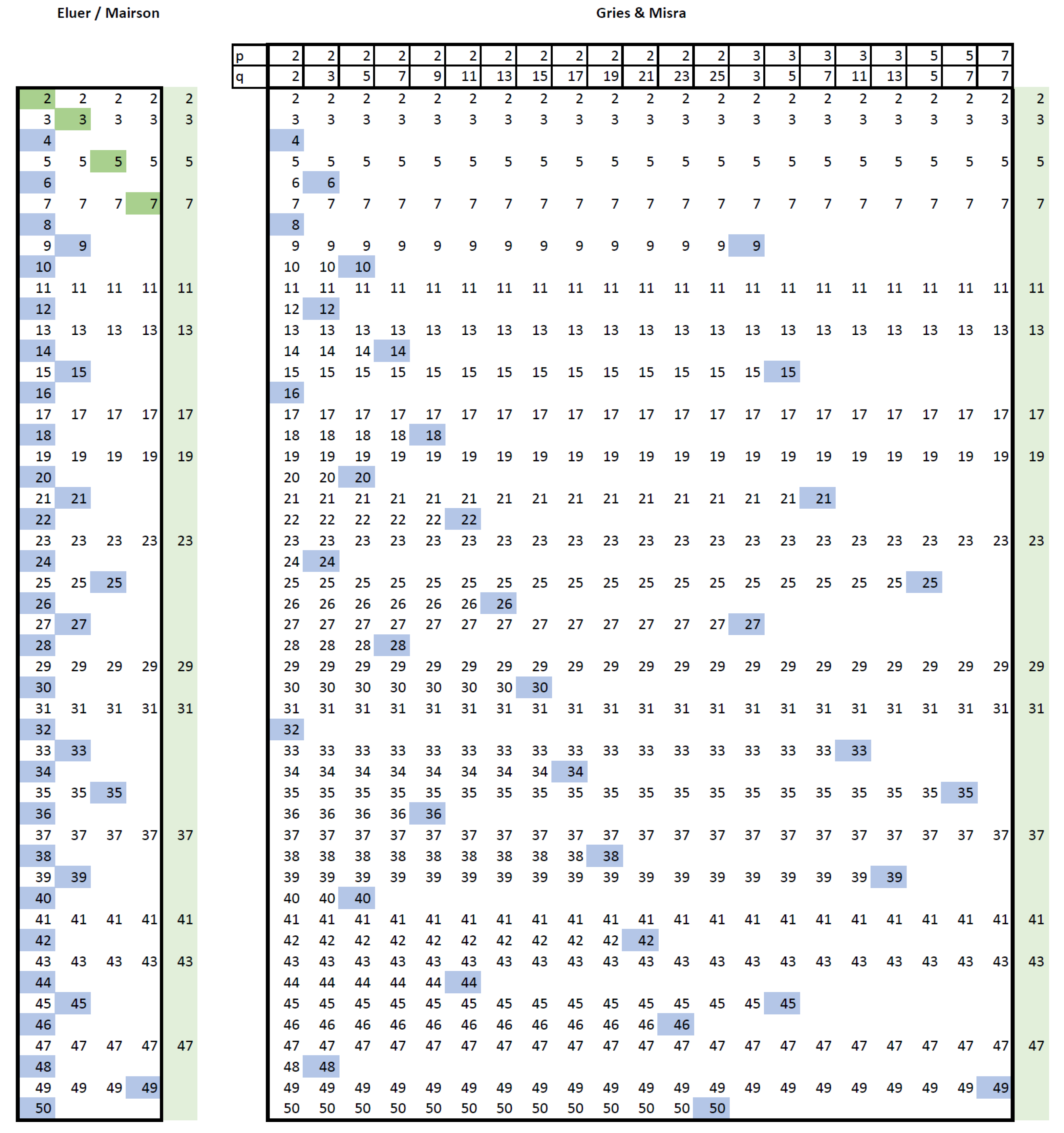
Mairson’s 1977 article introduces an algorithm using an intricate data structure based on a triple vector representation of a double linked list and strives to compute each composite only once. The algorithm is very similar to SoE+, as you can see in Figure 2. It is not clear if Mairson knew about Euler’s sieve—in any case, this is not mentioned in the paper. Mairson claimed a sub-linear time complexity for his algorithm; however, in practice, the memory complexity is very high and the performance is not optimal, as shown in Table 3. 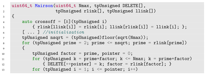The basic operations used to identify the composites may have O$\left(N\right)$; but when these operations are considered together with all the overhead necessary to maintain the relatively complex data structure, the things get rapidly out of control—see Algorithm 7 (function Mairson in the accompanying code offers an accurate rendition of the algorithm).

Figure 2. Combing techniques ($N_{max}=50$): in each iteration (column) the blue values are struck out.

Figure 2. Combing techniques ($N_{max}=50$): in each iteration (column) the blue values are struck out.

Algorithm 7 Mairson’s “sub-linear” sieve

llink is only necessary for crossof, but still required in this version of the algorithm To remain faithful, the implementation used here keeps the 1-based indexes

To optimize the memory footprint, Misra [25] proposes to eliminate multiples in reverse order, thus avoiding the need for a third vector (Pritchard later used this idea for his sieve). However, finding the start position (the position of the first value to eliminate) has a serious negative impact on the processing time, which we value the most.

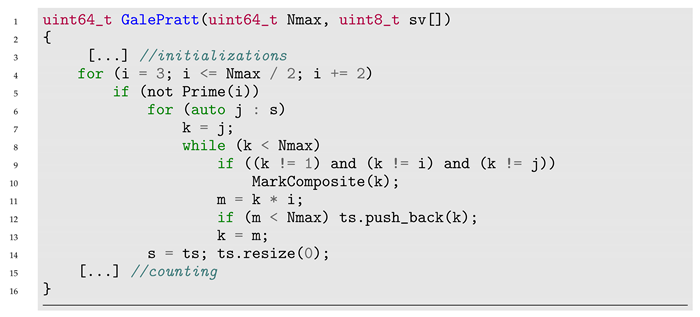
In the same year as Mairson, V. Pratt published a paper [23] about MACLISP/CGOL, where he proposes, as an example, another linear sieve, credited to Ross Gale and Vaughan Pratt. The logic behind this sieve is a little more convoluted—for each prime p, it strikes out composites formed by the powers of p and all reasonable composites stricken out in the previous iteration(s). The substance of the algorithm is presented in Algorithm 8.

Algorithm 8 Gale and Pratt sieve

The management of the lists can be quite taxing; Here is the first practical occurrence of the bit coding technique, as indicated by Singleton:

The sieve packs information at the bit level and skips all even candidates, thus a respectable performance and a relatively good memory footprint are obtained from the start. An updated but accurate version of this algorithm, translated into C++, can be found in the accompanying code (function GalePratt).

Another version of SoE+ was published [24] by Gries/Misra the following year, capitalizing on the work of Mairson. Mairson’s sieve was advertised as linear, but practice proved it to be much less efficient than 357. Gries/Misra had a similar idea for sifting primes through candidates and strove to achieve linearity by proposing a streamlined technique to manage the data. The sieve is also reminiscent of that of Gale/Pratt, processing composites formed by powers of the current p. While Mairson iterates for each first number p left in the list and strikes out the products between p and every number left in the list at that point, Gries/Misra iterate for each first number p left in the list and strike out the products between all powers of p and the next numbers in the list.

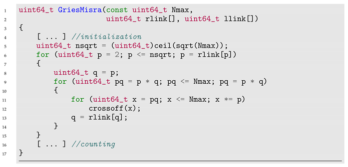
Figure 2 depicts the steps of Mairson vs. Gries/Misra primes combing algorithms. Each column contains all the numbers remaining in that step, with those marked for deletion highlighted blue. Both techniques strike out each composite exactly once, hence the basic linear character of the algorithms, but Mairson may strike out numbers that are to be used later in the same iteration, leading to more complications in data management to preserve the numbers that are marked until the end of the current cycle. Moreover, Gries/Misra eliminate the need for the third vector, lowering the memory requirements: see Algorithm 9 (all the details are provided in the accompanying code).

Algorithm 9 Gries/Misra linear sieve

The skeleton is very similar to Mairson

The same article [24] includes a discussion regarding the underlying data structure, showing how one can substitute a pointers vector with a vector of booleans to achieve further memory savings. Due to the great similarity between the two, these optimizations can also be applied to Mairson.

In theory, Gries/Misra should perform marginally better, because the same number of composites are removed and data management is simpler—in practice, because Gries/Misra has much worse locality (fewer composites are identified per cycle, so a lot of cache is trashed), Mairson performs better.

The next big thing in prime sieving appeared in 1981, in a paper from Paul Pritchard, introducing what is probably the most beautiful prime sieving algorithm: Wheel of Pritchard (SoP) [26]. The algorithm was further clarified by the author in [27]. SoP technique is derived from Mairson’s, except it does not parse the whole set of candidates for each p to eliminate multiples, but instead tries to iteratively and incrementally generate the smallest possible set of candidates to work on. In order to understand the algorithm, we need to recap some basic mathematical ideas:

• The product of the first n primes is called Primorial:

  $$P\left(n\right)=\prod _{i=1}^n{p}_i(\leftarrow p_1=2,p_2=3,\dots p_i\mathrm{is}\mathrm{prime})$$

  (9)
• If $\delta$ is coprime with any $p_i$, then $P\left(n\right)+\delta$ is also coprime with any $p_i$.

Let us construct a set (wheel) $S_n$ with all $\delta <P\left(n\right)$, where $\delta$ is coprime with all primes $p_i$ for $i<n$. First, it is evident that any $p_i$ is coprime with any other $p_j$, so we can use these as values for $\delta$. Thus, it is clear that any $p=kP\left(n\right)+\delta$ will remain coprime with all $p_i$. Extending this to all such p where $p<P(n+1)$ and then removing all multiples of $p_n$ will give us the new $S_{n+1}$, hence the iterative algorithm used to generate primes. Unfortunately, $P\left(n\right)$ increases very steeply with n, so it is very hard to create a table representation of the algorithm progression. Nevertheless, one can find some very intuitive animation for the Wheel of Pritchard on the internet, for example, at https://en.wikipedia.org/wiki/Sieve_of_Pritchard (accessed on 24 March 2024).

The next step is to construct a data structure that is clever enough not to destroy the performance of the sieve. Pritchard’s idea is to use a single vector s that keeps all identified $p_i$ in the lower part, and in the rest of the structure, the current $s_i$ − s combines both $rlink$ and $llink$ from a double linked list in one vector, capitalizing on the fact that, except 2, even numbers are not prime, so $s\left[i\right]$ will be $rlink\left[i\right]$ and $s[i-1]$ will be $llink\left[i\right]$. See Algorithm 10 and accompanying code for details.

Algorithm 10 Sieve of Pritchard

In each iteration, the muliples of current p are deleted in reverse order to avoid the need for an extra vector for that information.

The theoretical complexity of SoP is sublinear: O$\left(\frac{N}{\ln \ln N}\right)$, the best one achieved so far.

Pritchard published another meaningful and influential work in 1983 [28], which is important as it formalizes the so-called static or fixed wheel and proves the linear character of the sieve when a static wheel of the order $k=max\left(i\right|P\left(i\right)⩽\left(\sqrt{N}\right))$ is used (P is the Primorial). The results were somewhat refined by Sorenson in 1990 [29], and especially in [30,31]. Moreover, in 1991, Sorenson showed why SoE is still superior, in practice, to all other theoretically linear algorithms [32]. The timings for a basic but quite large (W8) fixed wheel SoE are given in Table 3—for small values of $N_{max}$, the total duration is penalized by the time that is necessary to generate the wheel; for middle values, a static wheel can be marginally more efficient than 357, but at very large values, it loses efficiency. To recover, the wheel size must be increased, which adds to the total duration and so on.

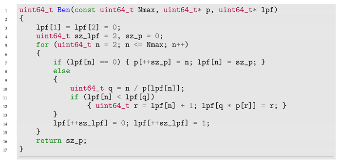
Several years passed before the next attempt to create something innovative: in 1986, Bengelloun [33] tried to address the problem that all the linear algorithms to date have a fixed superior limit $N_{max}$ up to which they compute the primes, meaning that if you want to find the next prime number that is greater than $N_{max}$, you will have to restart the process with another max value, which may not be very convenient. To resolve this, Bengelloun keeps track of the lowest prime factor ($lpf$) of composites in a vector that increases incrementally with n—each number is tested against the previous data, so, theoretically, the algorithm could continue ad infinitum. Unfortunately, the performance is not at all satisfactory for large numbers, but the idea is quite beautiful in its simplicity and is worth mentioning: for each odd composite, another, greater composite is stroked out. The underlying idea is that any composite n can be expressed as $n=p\times q$, where p is the lowest prime factor of n. Then, after obtaining, $p_{next}=$ the immediate next prime greater than p, the number $n_{next}=p_{next}\times q$, is struck out by inscribing $p_{next}$ in the $lpf$ vector at position $n_{next}$. See Algorithm 11 and accompanying code for details.

Algorithm 11 Bengelloun Continuous Incremental Primal Sieve

The locality is not the best, and the divisions and multiplications in lines 10 and 12 further impair the performance.

This incremental sieve was improved by Pritchard in 1994 [34], and transformed in a incremental additive and sub-linear sieve using wheels.

In 1987, Paul Pritchard performed an interesting analysis [35] of the linear algorithms found so far and synthesized them all by generalizing families of variations in the generic process of eliminating composites c, with two general expressions:

• based on least prime factor: $c=p\times f$ , where $p=$lpf$\left(c\right)$ (from this family, Mairson, Gries/Misra, SoP, and Bengelloun can be derived, but also two new siblings—called simply 3.2 and 3.3—with the same linear character);
• based on greatest prime factor: $c=p\times f$ , where $p=$gpf$\left(c\right)$ (from this family, Gale and Pratt can be derived, but also two new siblings—called 4.3 and 4.4—with the same linear character).

Finally, in 2003, we received a new, completely different type of sieve: a quadratic sieve—Sieve of Atkin (SoA) [36]—which has a theoretical complexity equal to SoP. (An interesting fact is that SoA was cited by Galway [37] in 2000, some years before the official publication; Galway referenced a paper of Atkin/Bernstein from 1999, and the URL cited by Galway for that paper— http://pobox.com/~djb/papers/primesieves.dvi—accessed on 10 April 2024).

SoA is based on the mathematical properties of some quadratic forms, thus being more related to SoS than SoE. It is quite promising, but relatively boring from the algorithmic perspective in its basic implementation. It capitalizes on the fact that all the numbers $p=12k+d$ that (a) have an odd number of positive solutions at these equations:

• $p=4x^2+y^2$, where d = 1 or 5, x and $y>0$
• $p=3x^2+y^2$, where d = 7, x and $y>0$
• $p=3x^2-y^2$, where d = 11, $x>y>0$

and (b) are squarefree (not a multiple of a square) are primes (in the original paper, one can find the justification for these properties, based on some more general $p=60k+d$ considerations). Frequent modulos and multiplications impair the performance, but the results are quite decent. See Algorithm 12 and function Atkin in the accompanying code for further details).

Algorithm 12 Sieve of Atkin

Initialize a sieve vector For all eligible pairs (x,y) mark the values of the quadratic forms in the vector Remove from the vector all values corresponding to: (a) even number of solutions (b) multiples of squares Count or otherwise use the primes indicated by the vector

The original technique is somewhat improved by Galway in [37], where the sieve is further segmented. Also, in [38], one can find some other interesting theoretical considerations regarding SoA.

Table 3 presents single-threaded timings for all these algorithms, including 357 as a baseline:

Table 3. Timings (ms) for linear and sub-linear algorithms.

N	$\mathit{\pi }\left(\mathit{N}\right)$	Algorithms
		Mairson	Gale/Pratt	Gries/Misra	Pritchard	Bengelloun	Atkin	W8 SoE	357
${10}^5$	9592	1	1	1	1	1	1	24	-
${10}^6$	78,498	8	4	9	4	9	4	26	2
${10}^7$	664,579	189	35	207	107	110	43	32	19
${10}^8$	5,761,455	1768	391	2204	1230	1336	796	167	174
${10}^9$	50,847,534	22,351	9615	24,143	15,738	13,761	9035	1771	1707
${10}^{10}$	455,052,511	-	-	-	-	-	125,367	22,968	18,415

Table 3. Timings (ms) for linear and sub-linear algorithms.

N	$\mathit{\pi }\left(\mathit{N}\right)$	Algorithms
		Mairson	Gale/Pratt	Gries/Misra	Pritchard	Bengelloun	Atkin	W8 SoE	357
${10}^5$	9592	1	1	1	1	1	1	24	-
${10}^6$	78,498	8	4	9	4	9	4	26	2
${10}^7$	664,579	189	35	207	107	110	43	32	19
${10}^8$	5,761,455	1768	391	2204	1230	1336	796	167	174
${10}^9$	50,847,534	22,351	9615	24,143	15,738	13,761	9035	1771	1707
${10}^{10}$	455,052,511	-	-	-	-	-	125,367	22,968	18,415

In conclusion, all the sub-linear sieves were better than a basic SoE, but they still were not close to the incremental 357 that, on modern CPUs, will use the cache for important performance gains. SoP is very clever, but the complex data management overhead cancels out the gain in complexity; Bengelloun has very bad locality and uses divisions when it encounters composites, and this lowers the performance for big numbers, when primes become more and more scarce; Gale/Pratt was quite optimized from its inception, requires fewer operations to manage its data structure, and remains a good performer in its class of SoE-derived linear sieves, where only static wheels can save the day; Atkin is the best performer for large values, but still worse than 357.

3.3. Parallel

The first step towards parallelization was made by Singleton in 1969 through 357’s incremental mechanism, mentioned in Section 3.2.1—its goal was to save memory, but it is also straightforward to segment the data, establish some boundary conditions, and then process each segment separately.

One should also acknowledge the paper of Bays/Hudson from 1977 [39], which seems to be the first time that data segmentation is formally explained and detailed in relationship with prime generation. The authors provide appropriate boundary conditions for each data segment and formalized the technique: see Algorithm 13.

Algorithm 13 Bays/Hudson—First segmented sieve

Generation of primes up to $x=x_0+2k\Delta$ in two steps: (a) basic generation up to $x_0$; (b) k iterations on a segment of length $\Delta$ (as only odd values will be represented in$\Delta$) Strike out multiples of each $p_i$ in the set of root primes inside $\Delta$ from the start point $y=mo{d}_{p_i}(p_i-mo{d}_{p_i}[(x_0-p_i)/2])+1$ (boundary condition) For each j left intact in $\Delta$, $p=x_o+2(j-1)$ is prime (for 1-based indexes) The next iteration starts from $x_0=x_0+2\Delta$ (as odd numbers are skipped in $\Delta$)

Unfortunately, parallel processing was not yet very popular—like Singleton, the Bays/Hudson paper does not address parallelization and their goal was to optimize memory footprint in an iterative approach, similar to Singleton, but without the need to keep track of multiples between segments. This idea was again “optimized” for performance, creating something very similar to 357. It is not clear if they were aware of 357, as their Bibliography has only one entry (Knuth’s Art of Programming vol.II), so probably their work was independent of Singleton’s. Where Singleton created an incremental algorithm but did not made the next step to segmentation, Bays/Hudson created the foundation of a segmented algorithm but reverted it back to an incremental one—nevertheless, it was a little early for the parallelization potential of these ideas to emerge.

However, the idea of segmenting data was not new: it was mentioned, for example, as early as 1973 by Brent [40] for a practical application of prime number sieving, being used to generate primes up to $2.6\times {10}^{12}$ to study the gaps between successive primes. It is notable that the article also mentioned the usage of a bit representation for each number, instead of the didactic byte, as suggested by Singleton, but earlier than the practical example of Gale/Pratt.

An important work regarding segmentation was published by Pritchard in 1983 [28], where he presents a useful, linear technique to segment a sieve based on static wheels—nevertheless, again, the goal was to minimize memory requirements and not parallelization. The results were refined by Sorenson in 1990 [29].

An article from 1987 by Bokhari [41] talks about multiprocessing SoE, but employs a very naive version of parallelization: it does not segment the data, but launches one process for each root prime to strike out composites—instead of data parallelism, it uses some form of task parallelism, which is not really appropriate here, and requires a lot of synchronization. The goal of this exercise was to test a new hardware (Flex/32) and not to generate primes per se—still, we have to appreciate this as the first recorded attempt to parallelize a prime generator sieve.

Other works of that period are referenced in some articles and may have some interesting content, but we cannot find them anymore. These include Parallel sieve methods for generating prime numbers (1980) by Tokyo Daigaku, T. Hikita, S. Kawai, Parallel speedup of sequential prime number sieves (1981) by Ian Parberry, or Massively Parallel Mathematical Sieves by Montry.

In 1994, Sorenson [42] tried to address the problem of latency and provided two solutions—one for low and another for high communication latency. The first solution is based on Algorithm 3.3 from Pritchard [35] improved using a static wheel, as in [28]—this is not a very useful idea in practice, as each worker will have to parse the whole $[2..N]$ data segment and then overlap all the results, like in [41]. The second version is more realistic, with a true data segmentation—the final step is to concatenate all data. This result is a formula that can compute the boundary conditions for each segment in the case of a static wheel.

In 2005 we found some attempts to parallelize SoP by Paillard [43,44], while in 2007 we found a coarse attempt to balance the load of a basic SoE in [45].

In the same year, Aziz et al. [46] used MPI to parallelize a sieve, but the “sieve” used in this work was a brute force (trial-division) algorithm. As in most papers regarding sieve parallelization, the main area of interest was not the sieve itself, but some practical or theoretical aspects linked to parallel computing, and the sieve was only used to demonstrate the problem and provide a possible solution. Similar, in 2010, there was an attempt by Bhukya et al. [47] to apply statistical DOE to SoE. Again, the article is more preoccupied with the methodology of efficiently deploying large-scale numerical applications on grid platforms than with SoE specifically.

When RAM is simply not enough, using another type of data repository can be quite taxing on performance—one can find some interesting insights regarding the I/O complexity of sieves in [48].

In addition to official studies, there was some activity in small communities of enthusiasts on the internet. There are notable active sieving projects that are currently looking for very large primes, like PrimeGrid (https://www.primegrid.com/, accessed on 10 April 2024) or GIMPS (https://www.mersenne.org/, accessed on 10 April 2024), but these efforts are not really about advancing systematic prime generation, which is the focus of this study.

The most interesting initiatives related to our domain are two very compelling projects hosted on GitHub, both implementing the segmented sieve of Eratosthenes:

(a)

primesieve (https://github.com/kimwalisch/primesieve, accessed on 10 April 2024)—a parallel CPU cache intensive generator;

(b)

CUDASieve (https://github.com/curtisseizert/CUDASieve, accessed on 10 April 2024)—a GPU accelerated C++/CUDA C fast sieve.

Both implementations use the so-called bucket list technique to store the root primes into lists of buckets: each list is associated with a segment, and a list contains only those primes that have multiples in that segment. The technique was devised by Tomás Oliveira e Silva [49], and was used in his project for Goldbach conjecture verification that reached $4\times {10}^{18}$ [50,51].

3.4. Other Sieve Variants

In 1965, P. Fischer [52] introduced an original idea: he theorized a one-dimensional iterative array of finite-state sequential machines that could represent a set of prime numbers. Fischer provided a solution to the problem, but also states that his solution is less efficient than SoE. Unfortunately, although the usage of such cellular automata for discrete prime number generation was explored in some papers, there was very little follow-up on this approach in order to achieve better efficiency for practical systematic prime generation. Some occasional references to this idea ([53,54,55]) appear to have mainly didactic purposes.

There were some tentative attempts to implement sieving using the functional programming paradigm [56,57,58] but these, too, seem more didactic in nature and exceed our scope and ambition.

Another category of sieves are those using some punctual primality tests, like AKS test in [59], which simply apply the test to all the numbers in the desired range. These include also examples like Sorenson [60], which uses the pseudosquares primality test, or Tarafder [61], which uses the Rabin–Miller test—this approach normally achieves a horrendous performance, as these tests are extremely complex. There were tentative attempts to compute the nth prime number, usually derived from generic formulas similar to Willans [62] as in [63,64]: again, these formulas are extremely complex and lead to horrific performance.

There are some alternatives that may merit more study: Robert Bennion’s “hopping sieve” ([65]), also detailed in [66]; the NPNG/FTF scheme from [67]; algorithms based on the divisibility of two consecutive numbers, like in [68,69]; techniques using Scheduling by Multiple Edge Reversal (SMER), like in [43,44].

The idea based on Diophantine approximation and Voronoi’s work on the Dirichlet divisor problem [70], from Harald Helfgott (the mathematician who proved Goldbach’s weak conjecture ) is also interesting.

4. Conclusions

The first sieving algorithm was published in 1961 by T.C. Wood, followed by contributions from B.A. Chartres and R. Singleton. H.G. Mairson, Gale/Pratt, and D. Gries/J. Misra worked oh linear sieves in the late 1970s, while C. Bays/R. Hudson introduced the segmentation technique for SoE. Paul Pritchard created his sub-linear sieve in the 1980s, and Jonathan Sorenson published several meaningful articles in the 1990s. The last major contribution was made in 2003 by Atkin/Bernstein, with Sieve of Atkin, which was born segmented and remains the practical sieve with the lowest theoretical complexity. No relevant algorithmic advances were identified after this, besides the optimization of parallelized SoE.

Most of the papers published since 2000 deal with the parallelization of SoE (and occasionally SoP), but these papers are quite narrow and mostly didactic in purpose—as if everybody agrees that there is nothing more to be said on this topic. Authors usually just apply newer hardware and software techniques to the old SoE, and the main focus is usually on the generic techniques and not the actual sieving algorithm.

4.1. A Sieve Taxonomy

A sieve classification may consider the following set of characteristics:

➪

Arithmetic complexity of the sieve:

➭

Sub-linear sieves—complexity is better than O$\left(N\right)$ (like SoP or SoA).

➭

Linear sieves—complexity is arround O$\left(N\right)$ (examples provided in Section 3.2.1).

➭

Slow sieves—performance degrades drastically with N (like trial-division or SoS).

➪

Space complexity of the sieve:

➭

Compact sieves—complexity is O$\left(\sqrt{N}\right)$ or better (incremental or segmented sieves).

➭

Normal sieves—complexity is around O$\left(N\right)$ (like simple SoE or the linear ones).

➭

Huge sieves—space requirements increase drastically with N (hopping sieve).

➪

Operations implied by the optimized algorithm:

➭

Additive sieves—only additions, subtractions and simple bit operations in the inner loop (like SoP).

➭

Regular sieves—some multiplications allowed in the inner loop (like Mairson, Singleton, etc.).

➭

Complex sieves—all operations: division, modulo etc. (trial division, basic SoA and Bengelloun, etc.).

➪

The end condition of the sieve:

➭

Perpetual sieves—given appropriate resources, it can run forever without resetting the calculus (357, Bengelloun).

➭

Caped sieves—can compute primes up a certain limit; changing the limit implies complex re-adjustments (almost all others).

➪

The availability of the results:

➭

Incremental sieves—iterations are relatively short and each iteration produces the next one or more prime numbers based on the results of the previous iteration (Chartres, Singleton, Bengelloun).

➭

Solid sieves—the whole set of primes is produced in one or a relatively small number of big, unrelated batches (almost all others).

➪

The treatment of the set of candidates:

➭

Integral sieves—the algorithm works on the whole set at once, or on a small number of very big batches in a certain order (basically all the sieves are born and initially presented as solid sieves; many are now segmented, but for some sieves like Mairson no segmentation technique was discovered).

➭

Segmented sieves—the algorithm works on a relatively large number of small, unrelated subsets of the whole dataset, in an arbitrary order (segmented algorithms are usually an adaptation of solid sieves—most algorithms are not initially segmented, although some, like SoA, may be presented from the start in their segmented version).

Of course, the goal would be to obtain a strongly sub-linear, compact, additive, perpetual, incremental and segmented sieve.

There are also other criteria that should be noted:

• How the candidates are produced: start from the full set of numbers in the interval of interest (practically all sieves apart SoP) or generate, from the beginning, a drastically reduced set of candidates that may considerably limit the volume of work (like SoP and static-wheel-based SoE);
• The goal is to simply count the primes, or to effectively generate the prime numbers—if the latter, consider whether they will be produced in order;
• The criteria used to eliminate composites: whether they are based on multiples of root primes (like SoE and most of the others), or on more complex polynomial expressions (like SoS or SoA).

4.2. Perspectives

A contiguous list of primes up to $2^{64}$ could further advance prime number theory, providing valuable insights into prime distribution and patterns, and would allow for primes to be generated in any interval up to $2^{128}$ (reaching the $2^{128}$ barrier will provide us with access to $2^{256}$ ranges, etc.). However, the sad reality is that we can now pragmatically and routinely produce very large discrete prime numbers, but we are not able to systematically generate in reasonable time all the prime numbers that our 64 bit processors can manage natively. Given the latest advances in both CPU and GPU power, perhaps it is time to re-ignite the ambition to refine existing, or create new, algorithms for the systematic generation of prime numbers in continuous sequence.

Generally speaking, the problem of systematically generating prime numbers is tackled by choosing a specific theoretical algorithm and optimally implementing it using the hardware at hand, using several possible approaches:

• Refine existing algorithms—simplify and reduce the theoretical/practical time and space complexity;
• Optimize implementation—establish better techniques based on the underlying hardware technologies at hand;
• Produce innovative algorithms—create new sieving schemes with potential for better arithmetic or binary complexity than the current ones.

Sieving algorithms were devised quite a long time ago, and most of them are now forgotten. The progress in this area has been almost abandoned in the last 20 years—we should reignite the work on optimizing at least the most promising of these algorithms by capitalizing on the latest insights and advances in computer science. A secondary goal would be to compute higher-order primes using lower-order numbers—i.e., producing 128-bit primes using 64-bit operands.

Optimal implementations should differ based on the underlying hardware technology that is involved. The approaches may be quite different to allow for various types of hardware bases to be optimally used:

• Local computing device—modern standards often surpass the resources of the 1990s mainframe computer: cache locality is paramount here, coupled with some parallelism;
• Individual computing equipment of server class—multiple hardware cores and terabytes of RAM require intensive parallelism plus cache locality;
• Local devices for parallel computing (GPUs, FPGAs etc.) contain thousands of hardware cores but limited RAM. These require massive parallelism plus cache locality and optimal usage of device memory; the orchestration/load-balancing of multiple local workers, and the latency of communication between host and workers should be considered;
• Distributed computing on modern server clusters—massive intensive parallelism coupled with cache locality, leading to issues like I/O and orchestration/load-balancing.

Regarding innovative algorithms, we have mentioned approaches like functional programming or cellular automata: it is not clear if a breakthrough is even possible in these directions, but further study is warranted in this area. The situation is similar in quantum computing: the challenge of creating continuous sequences of prime numbers within this framework has not yet been clearly defined, let alone resolved.

It is evident that, if more specialists would enter the field, there are enough areas of study for all—the authors of this report are mainly focused on algorithm refinement and the optimized implementation of established algorithms, with and without GPUs.