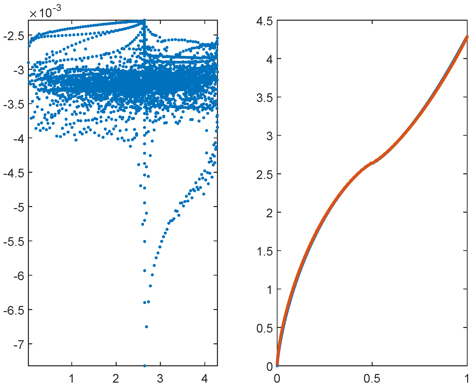
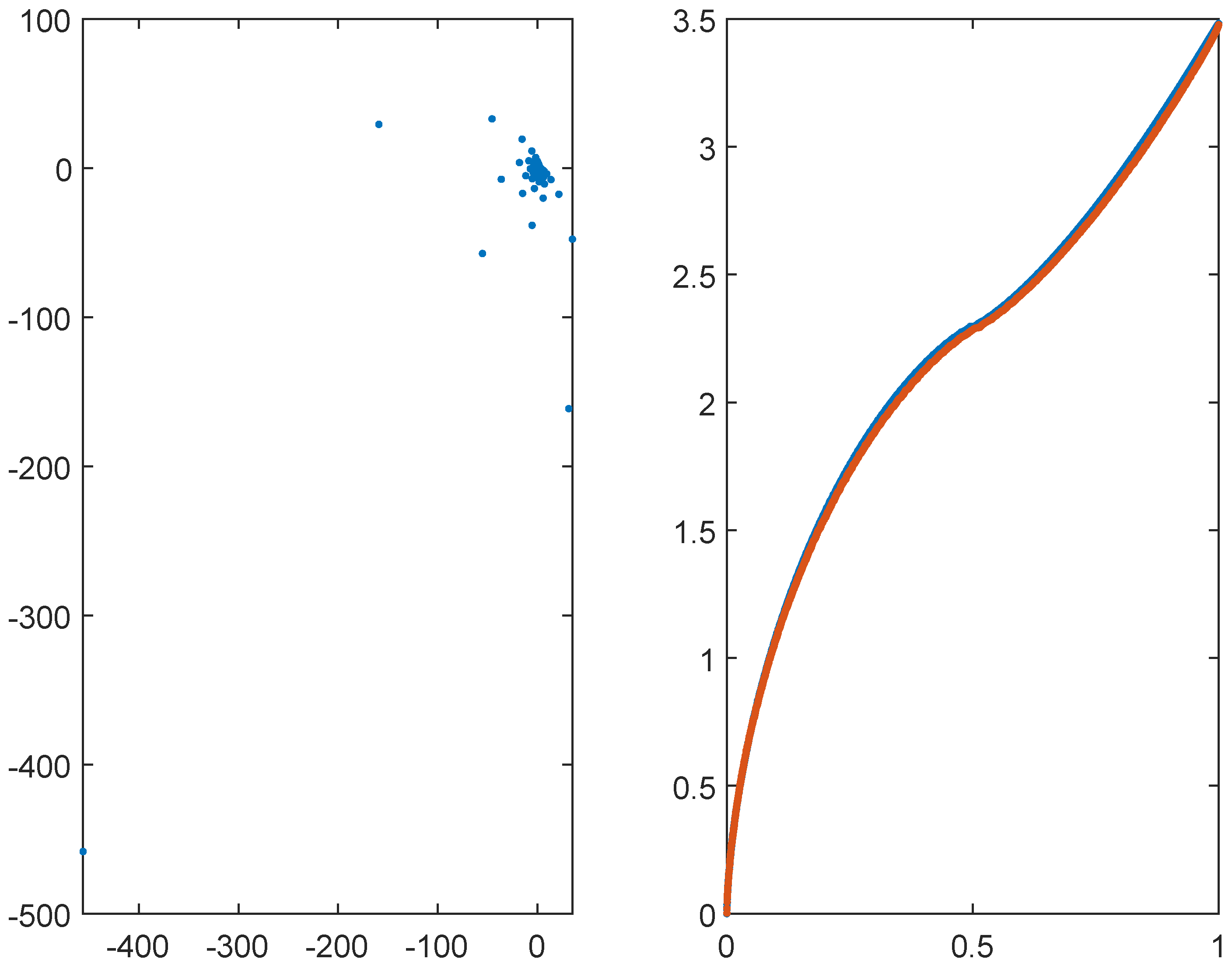
Figure 1.
Eigenvalues of the matrix for , and . The left panel reports the eigenvalues in the complex plane. The right panel reports in blue the real part of the eigenvalues and in red the equispaced samplings of in nondecreasing order, in the interval .
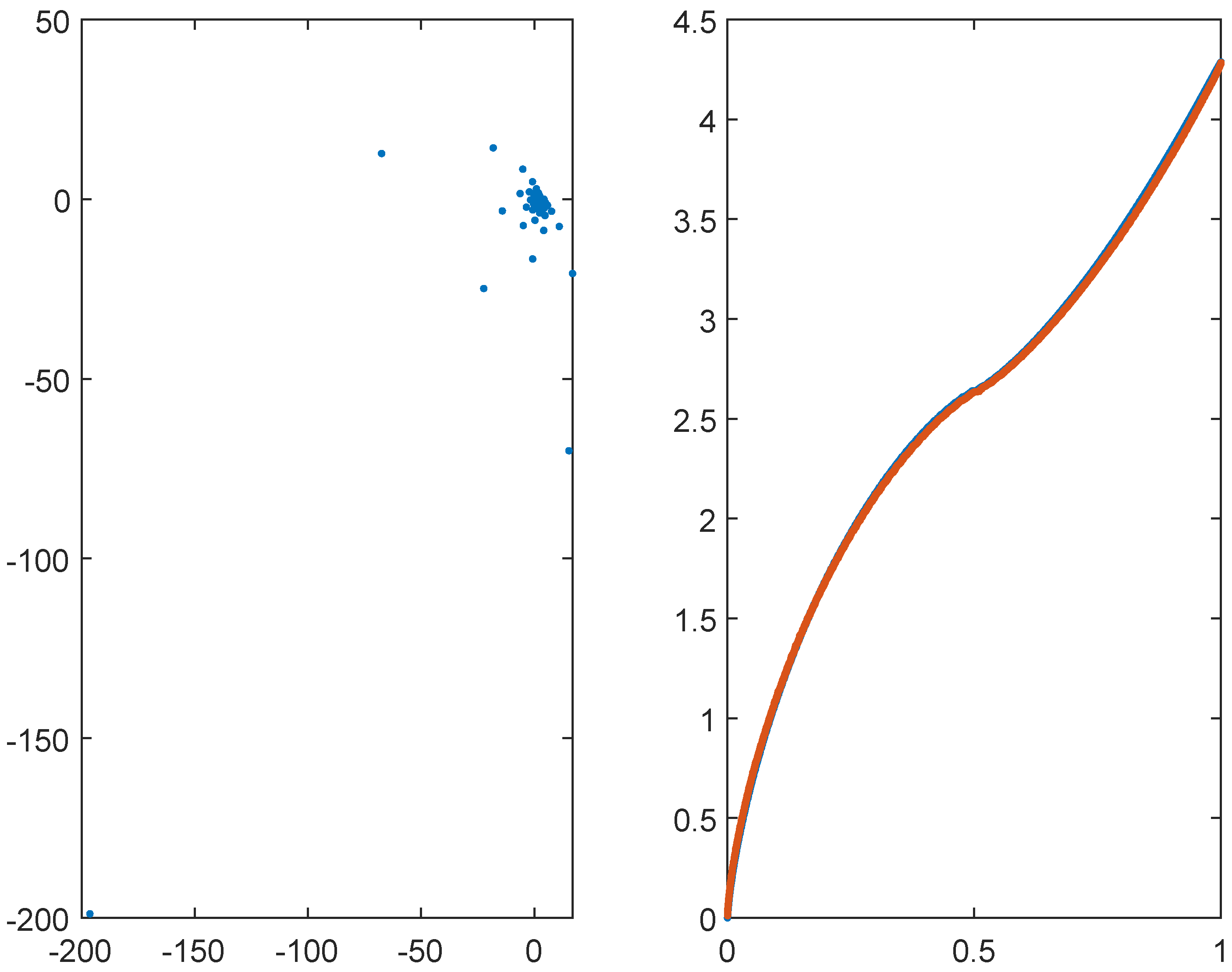
Figure 1.
Eigenvalues of the matrix for , and . The left panel reports the eigenvalues in the complex plane. The right panel reports in blue the real part of the eigenvalues and in red the equispaced samplings of in nondecreasing order, in the interval .
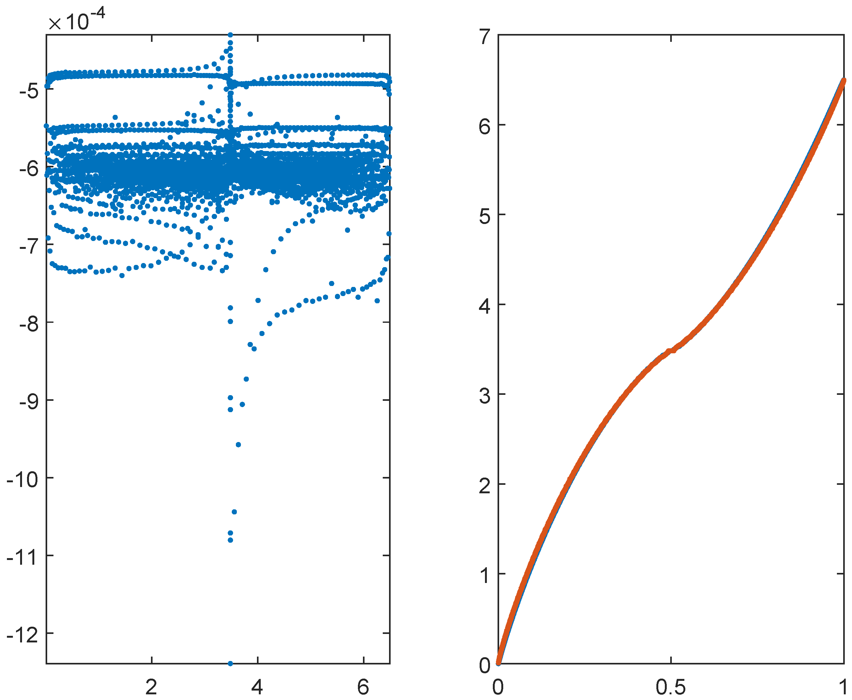
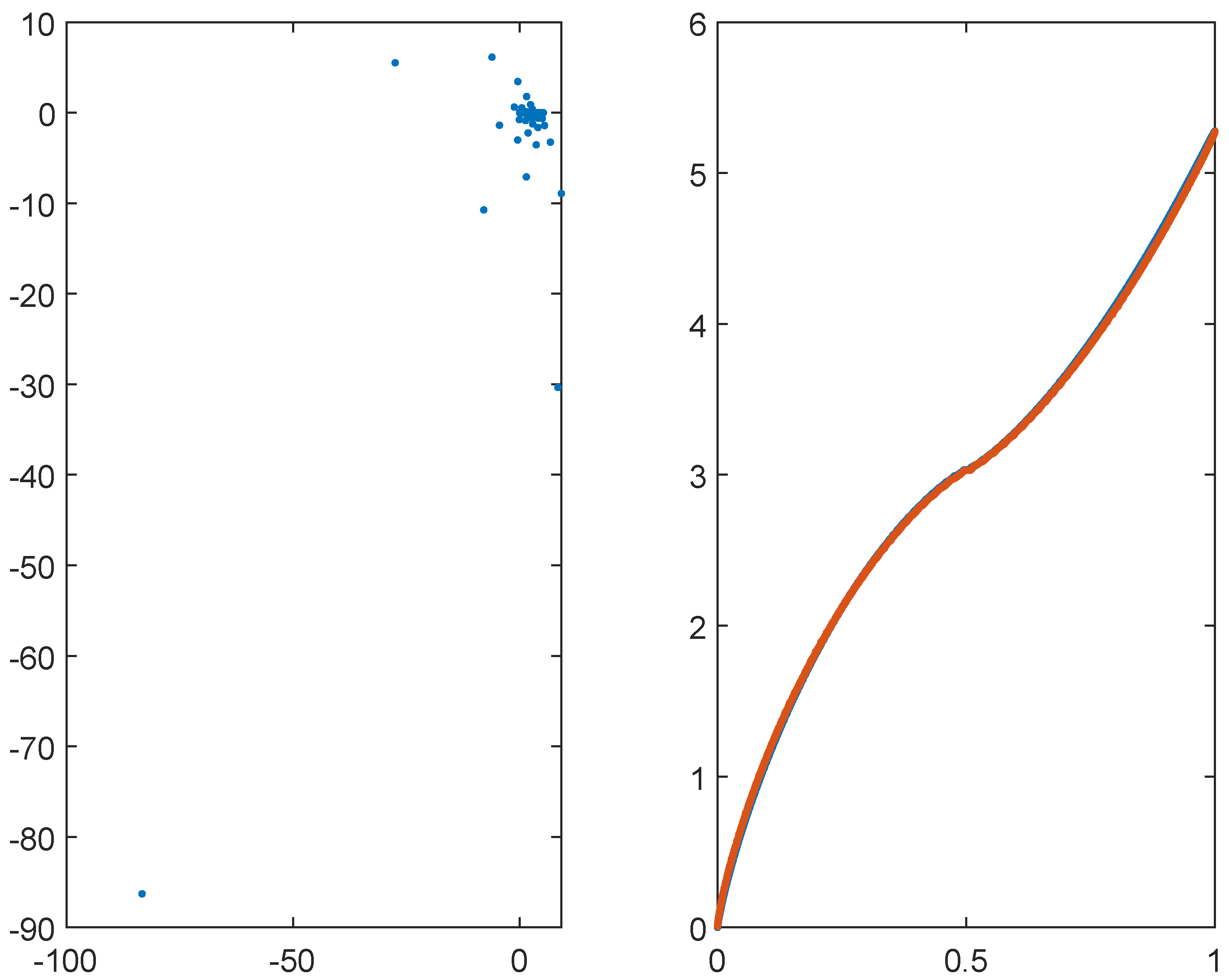
Figure 2.
Eigenvalues of the matrix for , and . The left panel reports the eigenvalues in the complex plane. The right panel reports in blue the real part of the eigenvalues and in red the equispaced samplings of in nondecreasing order, in the interval .
Figure 2.
Eigenvalues of the matrix for , and . The left panel reports the eigenvalues in the complex plane. The right panel reports in blue the real part of the eigenvalues and in red the equispaced samplings of in nondecreasing order, in the interval .
Figure 3.
Eigenvalues of the matrix for , and . The left panel reports the eigenvalues in the complex plane. The right panel reports in blue the real part of the eigenvalues and in red the equispaced samplings of in nondecreasing order, in the interval .
Figure 3.
Eigenvalues of the matrix for , and . The left panel reports the eigenvalues in the complex plane. The right panel reports in blue the real part of the eigenvalues and in red the equispaced samplings of in nondecreasing order, in the interval .
Figure 4.
Eigenvalues of the matrix for , and . The left panel reports the eigenvalues in the complex plane. The right panel reports in blue the real part of the eigenvalues and in red the equispaced samplings of in nondecreasing order, in the interval .
Figure 4.
Eigenvalues of the matrix for , and . The left panel reports the eigenvalues in the complex plane. The right panel reports in blue the real part of the eigenvalues and in red the equispaced samplings of in nondecreasing order, in the interval .
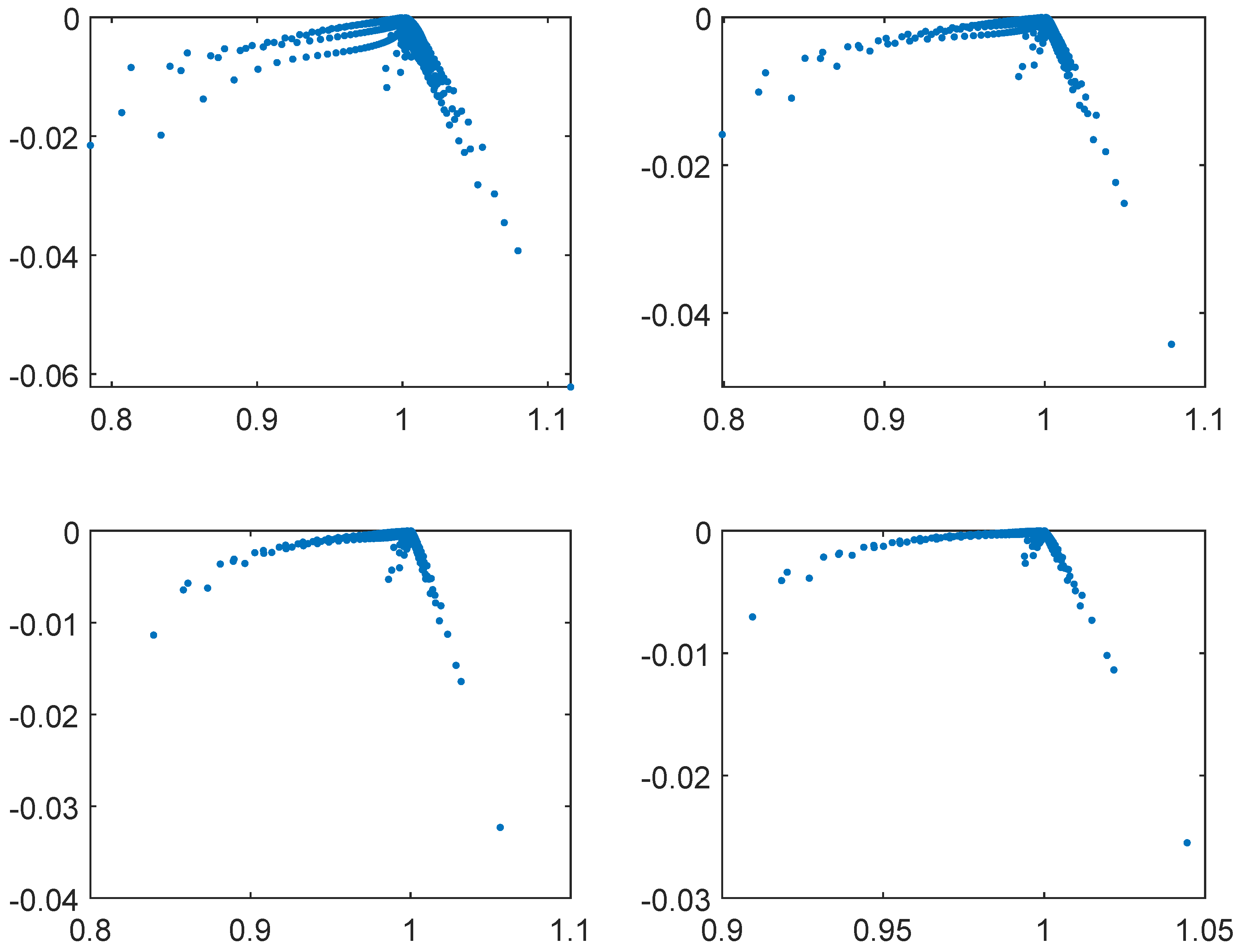
Figure 5.
Eigenvalues of the preconditioned matrix of size for and , respectively.
Figure 5.
Eigenvalues of the preconditioned matrix of size for and , respectively.
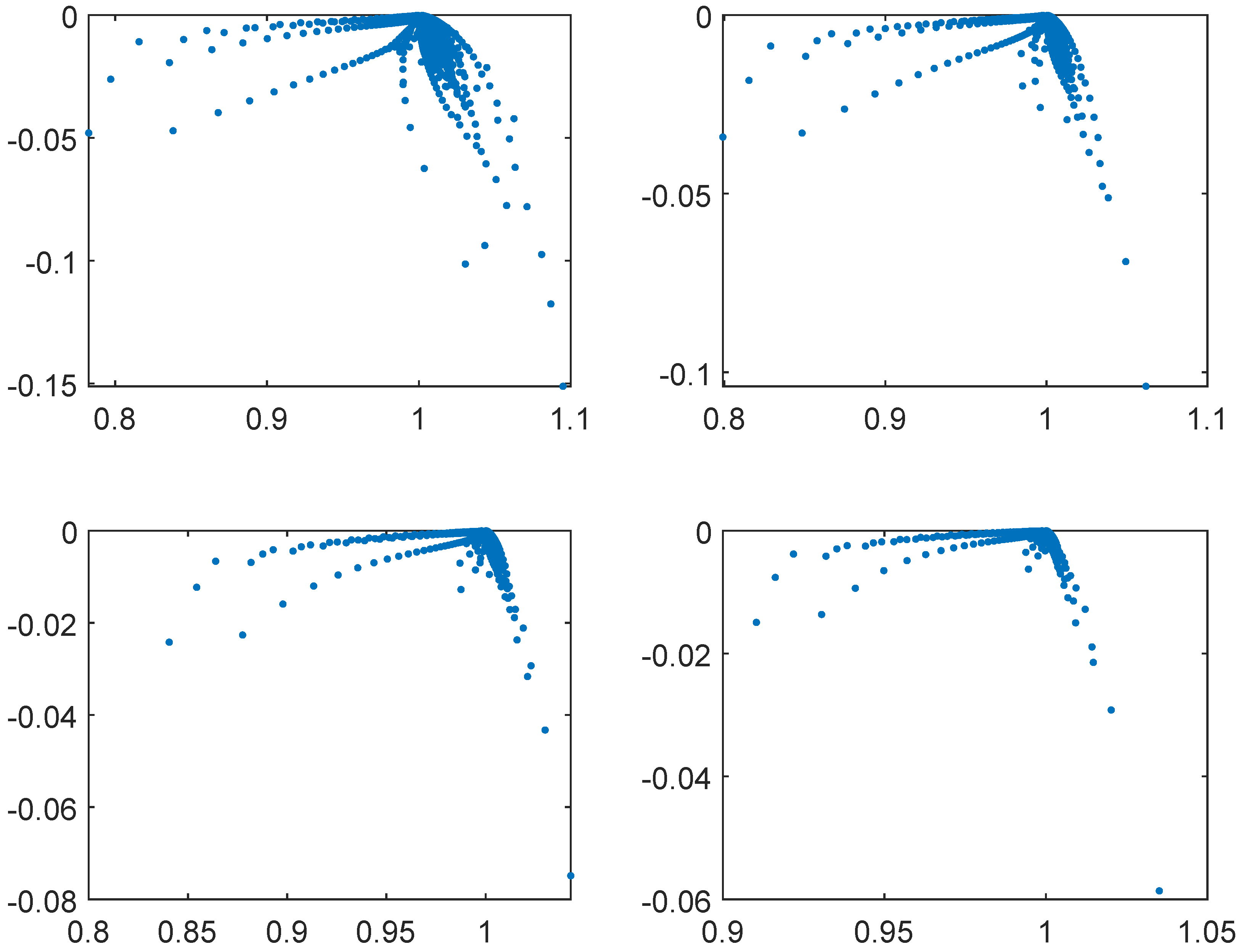
Figure 6.
Eigenvalues of the preconditioned matrix of size for and , respectively.
Figure 6.
Eigenvalues of the preconditioned matrix of size for and , respectively.
Figure 7.
Eigenvalues of the preconditioned matrix of size for and , respectively.
Figure 7.
Eigenvalues of the preconditioned matrix of size for and , respectively.
Figure 8.
Eigenvalues of the preconditioned matrix of size for and , respectively.
Figure 8.
Eigenvalues of the preconditioned matrix of size for and , respectively.
Figure 9.
Eigenvalues of the matrix for , and . The left panel reports the eigenvalues in the complex plane. The right panel reports in blue the real part of the eigenvalues and in red the equispaced samplings of in nondecreasing order, in the interval .
Figure 9.
Eigenvalues of the matrix for , and . The left panel reports the eigenvalues in the complex plane. The right panel reports in blue the real part of the eigenvalues and in red the equispaced samplings of in nondecreasing order, in the interval .
Figure 10.
Eigenvalues of the matrix for , and . The left panel reports the eigenvalues in the complex plane. The right panel reports in blue the real part of the eigenvalues and in red the equispaced samplings of in nondecreasing order, in the interval .
Figure 10.
Eigenvalues of the matrix for , and . The left panel reports the eigenvalues in the complex plane. The right panel reports in blue the real part of the eigenvalues and in red the equispaced samplings of in nondecreasing order, in the interval .
Figure 11.
Eigenvalues of the matrix for , and . The left panel reports the eigenvalues in the complex plane. The right panel reports in blue the real part of the eigenvalues and in red the equispaced samplings of in nondecreasing order, in the interval .
Figure 11.
Eigenvalues of the matrix for , and . The left panel reports the eigenvalues in the complex plane. The right panel reports in blue the real part of the eigenvalues and in red the equispaced samplings of in nondecreasing order, in the interval .
Figure 12.
Eigenvalues of the matrix for , and . The left panel reports the eigenvalues in the complex plane. The right panel reports in blue the real part of the eigenvalues and in red the equispaced samplings of in nondecreasing order, in the interval .
Figure 12.
Eigenvalues of the matrix for , and . The left panel reports the eigenvalues in the complex plane. The right panel reports in blue the real part of the eigenvalues and in red the equispaced samplings of in nondecreasing order, in the interval .
Figure 13.
Eigenvalues of the preconditioned matrix of size for and .
Figure 13.
Eigenvalues of the preconditioned matrix of size for and .
Table 1.
Number of outliers with respect to a neighborhood of 1 of radius or and related percentage for increasing dimension .
Table 1.
Number of outliers with respect to a neighborhood of 1 of radius or and related percentage for increasing dimension .
|
|---|
| | | | |
| | |
| 2 | | 227 | |
| 6 | | 302 | |
| 16 | | 307 | |
| | |
| 1 | | 89 | |
| 5 | | 99 | |
| 13 | | 154 | |
| | |
| 0 | 0 | 35 | |
| 3 | | 60 | |
| 8 | | 112 | |
| | |
| 0 | 0 | 20 | |
| 0 | 0 | 38 | |
| 0 | 0 | 73 | |
Table 2.
Number of outliers with respect to a neighborhood of 1 of radius or and related percentage for increasing dimension .
Table 2.
Number of outliers with respect to a neighborhood of 1 of radius or and related percentage for increasing dimension .
|
|---|
| | | | |
| | |
| 3 | | 233 | |
| 7 | | 395 | |
| 16 | | 456 | |
| | |
| 2 | | 115 | |
| 6 | | 131 | |
| 15 | | 182 | |
| | |
| 0 | 0 | 46 | |
| 3 | | 66 | |
| 8 | | 116 | |
| | |
| 0 | 0 | 20 | |
| 0 | 0 | 39 | |
| 0 | 0 | 75 | |
Table 3.
Number of outliers with respect to a neighborhood of 1 of radius or and related percentage for increasing dimension .
Table 3.
Number of outliers with respect to a neighborhood of 1 of radius or and related percentage for increasing dimension .
|
|---|
| | | | |
| | |
| 8 | | 235 | |
| 11 | | 450 | |
| 22 | | 588 | |
| | |
| 2 | | 128 | 50 |
| 6 | | 164 | |
| 15 | | 217 | |
| | |
| 0 | 0 | 58 | |
| 2 | | 76 | |
| 8 | | 123 | |
| | |
| 0 | 0 | 27 | |
| 0 | 0 | 43 | |
| 0 | 0 | 78 | |
Table 4.
Number of outliers with respect to a neighborhood of 1 of radius or and related percentage for increasing dimension .
Table 4.
Number of outliers with respect to a neighborhood of 1 of radius or and related percentage for increasing dimension .
|
|---|
| | | | |
| | |
| 20 | | 237 | |
| 33 | | 547 | |
| 55 | | 923 | |
| | |
| 9 | | 154 | |
| 13 | | 246 | |
| 24 | | 367 | |
| | |
| 3 | | 78 | |
| 5 | | 117 | |
| 11 | | 181 | |
| | |
| 1 | | 42 | |
| 1 | | 61 | |
| 1 | | 97 | |
Table 5.
Maximal distance of eigenvalues of the preconditioned matrix from 1 for increasing dimension .
Table 5.
Maximal distance of eigenvalues of the preconditioned matrix from 1 for increasing dimension .
|
|---|
|
| n | | | | |
| | | | |
| | | | |
| | | | |
|
| n | | | | |
| | | | |
| | | | |
| | | | |
|
| n | | | | |
| | | | |
| | | | |
| | | | |
|
| n | | | | |
| | | | |
| | | | |
| | | | |
Table 6.
Number of preconditioned GMRES iterations to solve the linear system for increasing dimension till .
Table 6.
Number of preconditioned GMRES iterations to solve the linear system for increasing dimension till .
|
|---|
| | |
| | | | | |
| n | - | | - | | - | | - | |
| 35 | 9 | 41 | 8 | 47 | 7 | 54 | 7 |
| 54 | 9 | 67 | 9 | 83 | 8 | 101 | 7 |
| 82 | 10 | 109 | 9 | 144 | 8 | 189 | 7 |
| 124 | 11 | 177 | 10 | 251 | 9 | 351 | 7 |
| 189 | 11 | 288 | 10 | 437 | 9 | >500 | 8 |
| 287 | 11 | 467 | 10 | >500 | 9 | >500 | 8 |
| | |
| | | | | |
| n | - | | - | | - | | - | |
| 36 | 9 | 42 | 9 | 49 | 8 | 56 | 7 |
| 55 | 10 | 68 | 9 | 85 | 8 | 103 | 7 |
| 83 | 11 | 111 | 10 | 147 | 9 | 192 | 7 |
| 126 | 11 | 180 | 10 | 256 | 9 | 356 | 8 |
| 191 | 12 | 293 | 10 | 449 | 9 | >500 | 8 |
| 290 | 12 | 477 | 11 | >500 | 10 | >500 | 8 |
| | |
| | | | | |
| n | - | | - | | - | | - | |
| 36 | 10 | 42 | 9 | 49 | 8 | 56 | 7 |
| 55 | 11 | 69 | 10 | 86 | 9 | 104 | 7 |
| 84 | 11 | 112 | 10 | 148 | 9 | 193 | 8 |
| 127 | 12 | 182 | 10 | 258 | 9 | 359 | 8 |
| 193 | 12 | 295 | 11 | 452 | 10 | >500 | 8 |
| 293 | 12 | 480 | 11 | >500 | 10 | >500 | 8 |
| | |
| | | | | |
| n | - | | - | | - | | - | |
| 38 | 13 | 44 | 11 | 51 | 9 | 57 | 8 |
| 59 | 14 | 71 | 12 | 88 | 10 | 106 | 8 |
| 89 | 16 | 116 | 12 | 152 | 10 | 197 | 8 |
| 136 | 17 | 188 | 13 | 264 | 10 | 366 | 8 |
| 206 | 18 | 306 | 13 | 461 | 10 | >500 | 8 |
| 312 | 20 | 498 | 14 | >500 | 11 | >500 | 9 |
Table 7.
Number of outliers with respect to a neighborhood of 1 of radius or and related percentage for increasing dimension .
Table 7.
Number of outliers with respect to a neighborhood of 1 of radius or and related percentage for increasing dimension .
|
|---|
| | | | |
|---|
| | |
| 15 | | 85 | |
| 26 | | 162 | |
| 50 | | 303 | |
Table 8.
Number of preconditioned GMRES iterations to solve the linear system for increasing dimension till .
Table 8.
Number of preconditioned GMRES iterations to solve the linear system for increasing dimension till .
|
|---|
|
|---|
| n | - | |
| 69 | 17 |
| 125 | 22 |
| 236 | 32 |
| 454 | 47 |
| >500 | 70 |
| >500 | 108 |


