Vectorized Numerical Algorithms to Solve Internal Problems of Computational Fluid Dynamics

Abstract

The opportunities provided by new information technologies, object-oriented programming tools, and modern operating systems for solving boundary value problems in CFD described by partial differential equations are discussed. An approach to organizing vectorized calculations and implementing finite-difference methods for solving boundary value problems in CFD is considered. Vectorization in CFD problems, eliminating nested loops, is ensured through the appropriate data organization and the use of vectorized operations with arrays. The implementation of numerical algorithms with vectorized mesh structures, including access to internal and boundary mesh cells, is discussed. Specific examples are reported and the implementation of the developed computational algorithms is discussed. Despite the fact that the capabilities of the developed algorithms are illustrated by solving benchmark CFD problems, they enable a relatively simple generalization to more complex problems described by three-dimensional equations.

1. Introduction

Modern computational technologies are represented by general-purpose and subject-specific software packages. Research and modeling of multiphysics processes in technological systems is inextricably linked with the use of such technologies. The following ways to further improve performance are possible: parallelization at the algorithm level, which will lead to a reduction in the number of synchronization operations and lower costs for thread dispatching; and implementation on a specialized device (for example, GPGPU).

The development of models and algorithms for performing multivariant analysis of various structures at the stages of exploratory research, in which the efficiency of obtaining results plays an important role, is becoming quite important [1,2]. At the same time, a significant part of the computational resources is devoted to solving systems of linear algebraic equations (SAE), where about 40% of processor time is spent on solving SAE. The creation of algorithms that increase the efficiency of solving SAE is one of the main directions for increasing the performance of software packages. Vectorization of calculations is one of the promising optimization methods, along with the implementation of parallel computing algorithms [3,4].

Modern programming languages (for example, C++) enable creating vectorized algorithms, the effectiveness of which is evident with the appropriate hardware. Vectorization is one of the ways to perform parallel computing, in which the program is modified in a certain way to perform several similar operations simultaneously [5,6]. This approach potentially leads to a significant acceleration of similar calculations over large datasets. To improve program execution speed, MATLAB 5 uses loop vectorization, pre-allocation of arrays in memory, removal of unnecessary variables and functions, and memory defragmentation [7,8]. MATLAB capabilities for implementing parallel computing remain beyond the scope of many studies [9]. MATLAB-vectorized computations using large arrays may be good candidates for GPU acceleration [10,11].

Many problems in CFD, when mathematically modeled, are reduced to boundary value problems for systems of differential equations. Meanwhile, the numerical solution of the Cauchy problem is well formalized and provided by reliably developed methods for finding an approximate solution, and a wide range of these methods (Euler, Runge–Kutta, and others) are presented in many packages of computational mathematics (for example, MATLAB). Boundary value problems represent a more difficult object to study. Solving many of them requires an individual approach and selection of the most effective solution method [12,13].

The speed of an algorithm is critical in determining its reliability, particularly in real-time applications. To ensure that the algorithm runs as quickly as possible, it is important to use vectorized mathematical functions for fast operations on large arrays of data without the need for explicit loops. Programming languages (MATLAB/GNU Octave or Python) that implement vectors and matrices may have easy means for vectorization. Many operations are implemented in a way that eliminates the overhead of loops, pointer indirection, and per-element dynamic type checking. Loops in MATLAB are slower compared to languages such as C/C++; one of the reasons is MATLAB’s dynamically typed nature. During each iteration, MATLAB has to perform a series of checks, such as determining the type of variable, resolving its scope, and checking for invalid operations. In C/C++, arrays consist of one data type, which the compiler knows in advance. This is why loops in MATLAB are often slower than in C/C++, and nested loops can significantly slow down the performance.

Many CFD solution procedures are extensively used in solutions of Euler or Navier–Stokes equations. However, these procedures are computationally demanding. One reason for this is the slow convergence rates of the numerical relaxation algorithms that are commonly used. It is shown that the convergence rates are greatly enhanced by using multigrid methods with a conventional scalar processor [14].

The structure of numerical algorithms and their implementation on vector computers are widely discussed. There are many examples of vectorized numerical algorithms that enable improving performance of code running on modern CPUs. These examples include adaptive quadrature codes process [15], solution of linear algebraic equations [16,17], integration of ordinary differential equations [18], and convergence acceleration techniques [19]. Applications of various vectorized algorithms for solving CFD problems are reported in [20,21,22,23,24]. Modern GPUs provide additional possibilities for acceleration of computer codes, but their use requires algorithm adaptation to the memory structure [25].

The Godunov method is widely used for solving systems of unsteady equations of gas dynamics. In this method, at each iteration of calculations, the Riemann problem is solved on each face of each cell of the computational mesh to determine the fluxes through these faces. Due to the fact that the dimensions of the computational meshes used for calculations amount to tens and hundreds of millions of cells, the effective use of numerical methods with Riemann solvers requires the use of supercomputers and the use of various approaches regarding parallelization of calculations. The most low-level approach used to increase supercomputer application performance is code vectorization.

Numerical methods based on solving the Riemann problem on the decay of an arbitrary discontinuity are demanding on computing resources. The instruction sets of modern programming languages have a number of features that allow vectorization to be applied to the software context of the Riemann solver, which leads to significant speedup of the solver. Using an example of an exact Riemann solver, a practical approach to vectorizing program code for solving CFD problems, including simple linear sections and also nested loops, is considered. The exact Riemann solver has a compact implementation and accommodates a number of features of the software context that require their own techniques when performing vectorization. Examples are provided and implementation of the developed computational algorithms is discussed.

2. Governing Equations

Unsteady supersonic flows of inviscid compressible gas are considered. These flows are described by Euler equations. Finite volume method and time-marching scheme are applied to discretization of Euler equations. Euler equations are written for three independent variables, time, and two Cartesian coordinates. Generalization of governing equations for three Cartesian coordinates is straightforward.

Governing equations are written in conservative form as

$$\begin{array}{c}\hfill \frac{\partial \mathit{U}}{\partial t}+\frac{\partial \mathit{F}}{\partial x}+\frac{\partial \mathit{G}}{\partial y}=0,\end{array}$$

(1)

where t is the time, x and y are the Cartesian coordinates. Equation of state of perfect gas is

$$\begin{array}{c}\hfill p=(\gamma -1)\rho \epsilon .\end{array}$$

Total energy per unit volume is found as

$$\begin{array}{c}\hfill e=\rho \epsilon +\frac{1}{2}\rho (u^2+v^2).\end{array}$$

The vector of conservative variables, $\mathit{U}$, and the vectors of fluxes, $\mathit{F}$ and $\mathit{G}$, have the form

$$\begin{array}{c}\hfill \mathit{U}=\left(\begin{array}{c}\rho \\ \rho u\\ \rho v\\ e\end{array}\right),\mathit{F}=\left(\begin{array}{c}\rho u\\ \rho uu+p\\ \rho uv\\ (e+p)u\end{array}\right),\mathit{G}=\left(\begin{array}{c}\rho v\\ \rho uv\\ \rho vv+p\\ (e+p)v\end{array}\right).\end{array}$$

Here, $\rho$ is the density, u and v are the velocity components in Cartesian directions x and y, p is the pressure, e is the specific total energy and $\epsilon$ is the specific internal energy, and $\gamma$ is the ratio of specific heat capacities at constant pressure and constant volume. Euler equations and relevant initial and boundary conditions do not contain any non-dimensional parameters. Euler equations written in dimensional and non-dimensional variables have the same form.

Steady state flows are described with Euler Equation (1). In this case, it is assumed that flow is hyperbolic (velocity magnitude is larger than speed of sound, $u^2+v^2>c^2$) in one of the Cartesian directions. For example, hyperbolicity in x direction takes place if $u^2>c^2$.

3. Numerical Method

For simplicity, a two-dimensional Cartesian mesh is applied. Mesh step sizes in x and y directions are uniform. The value of the vector of conservative flow variables in the center of control volume is ${\mathit{U}}_{i,j}$, $i=1,2,\dots ,M$ and $i=1,2,\dots ,N$. A number of control volumes in x and y directions are M and N. The time step size is $\Delta t$. The mesh function is constant over control volume.

The numerical algorithm involves reconstruction of flow variables on the faces of control volumes using the averaged values of the vector of flow variables in the centers of control volumes. The reconstruction step is applied to physical variables. The Riemann problem is solved on each face of the control volume. Solutions of the Riemann problem on left and right faces of the control volume are ${\mathit{U}}_{i-1/2,j}$ and ${\mathit{U}}_{i+1/2,j}$. Application of the explicit time marching scheme and Godunov method leads to the numerical scheme

$$\begin{array}{c}\hfill \frac{{\mathit{U}}_{i,j}^{n+1}-{\mathit{U}}_{i,j}^n}{\Delta t}+\frac{{\mathit{F}}_{i+1/2,j}^n-{\mathit{F}}_{i-1/2,j}^n}{\Delta y}+\frac{{\mathit{G}}_{i,j+1/2}^n-{\mathit{G}}_{i,j-1/2}^n}{\Delta y}=0.\end{array}$$

(2)

The superscript $n=0,1,\dots$ is related to the time step.

The flux on the faces of control volume is linearized and found as

$$\begin{array}{c}\hfill {\mathit{F}}_{i+1/2,j}=\frac{1}{2}\left({\mathit{F}}_{i,j}^n+{\mathit{F}}_{i+1,j}^n\right)+\frac{1}{2}{\left|A\right|}_{i+1/2,j}^n\left({\mathit{F}}_{i,j}^n-{\mathit{F}}_{i+1,j}^n\right),\end{array}$$

where $A={(\partial \mathit{F}/\partial \mathit{U})}^{-1}$ is Jacobian.

The stability condition for Equation (1) is

$$\begin{array}{c}\hfill C=max|{\lambda }_{\pm }|\frac{\Delta x}{\Delta y}⩽1.\end{array}$$

Eigenvalues of the Jacobian are

$$\begin{array}{c}\hfill {\lambda }_{\pm }=\frac{uv\pm c{(u^2+v^2-c^2)}^{1/2}}{u^2-c^2}.\end{array}$$

The speed of sound is

$$\begin{array}{c}\hfill c={\left[(\gamma -1)h-\frac{1}{2}(\gamma -1)(u^2+v^2)\right]}^{1/2},\end{array}$$

where h is the total enthalpy.

A three-step Runge–Kutta scheme is applied to integration in time direction. Godunov method uses the analytical solution of the Riemann problem. The exact solution consists of two waves, a shock wave or a simple rarefaction, and a tangential discontinuity. These discontinuities are separated from each other by uniform flow zones. Numerical scheme (2) is the scheme of the first order of accuracy. Higher-order accuracy schemes are created using piece-wise distributions of flow quantities in the control volume and interpolation procedure to integrate Euler equations in marching direction.

4. Addressing Mesh Cells

A structured mesh covering the computational domain has a structure similar to a two-dimensional array. This allows to address the cells (or nodes) with two indices, i and j. A mesh node with indices $(i,j)$ has neighbors that are addressed, giving them increments or decrements.

4.1. Vectorization of Loops

Work with mesh structures is usually carried out with cyclic algorithms and nested loops. Using a pseudo programming language, this algorithm is written as

—one-dimensional case

•  for i=1 to nx step 1
•    begin
•      U(i)=...
•    end

—two-dimensional case

•  for i=1 to nx step 1
•    for j=1 to ny step 1
•      begin
•        U(i,j)=...
•      end

Here, nx and ny are number of nodes in x and y directions. This approach involves calculating an index expression to address the data and store the result in U array.

In solution of CFD problems in rectangular fluid domain, two-dimensional data structures correspond to Cartesian coordinates of mesh nodes and flow quantities, such as velocity components, pressure, and temperature. Multidimensional arrays in computer memory are stored as linear sequential structures, and the hardware capabilities of modern computer processor units make it possible to ensure high performance of computational algorithms with appropriate data organization.

Vectorization allows to work with data as a single structure, which not only makes the design of a computational algorithm compact, avoiding nested loops, but also increases the efficiency of calculations. Vectorization of calculations is organized with modern object-oriented programming languages like C++ or MATLAB.

4.2. Addressing to Internal Cells

Implementation of computational algorithms requires addressing to current cell or node and values in neighboring cells or nodes included in the finite-difference template. The traditional way to address flow quantities is to specify two indices defining line and column of two-dimensional array.

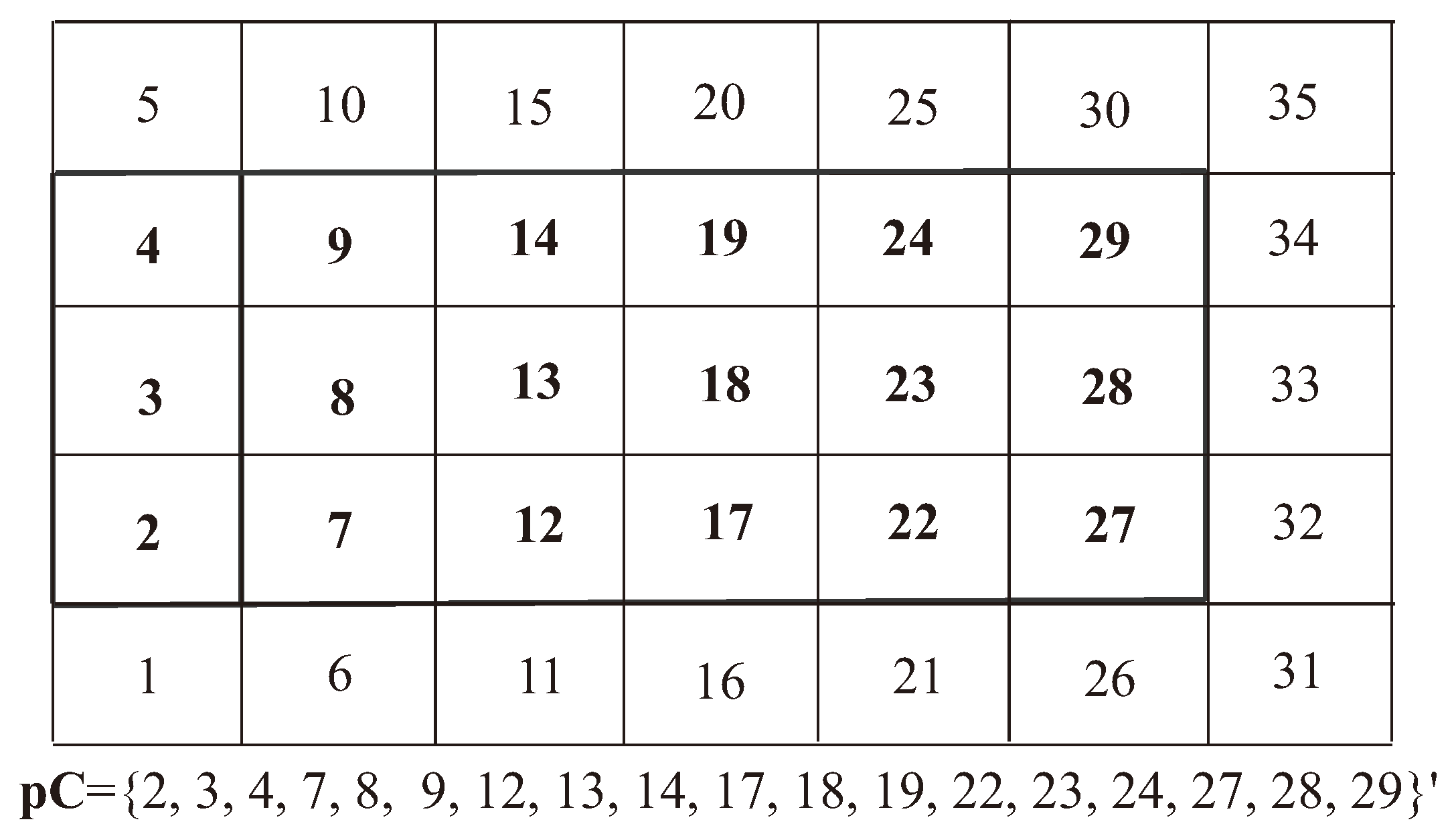
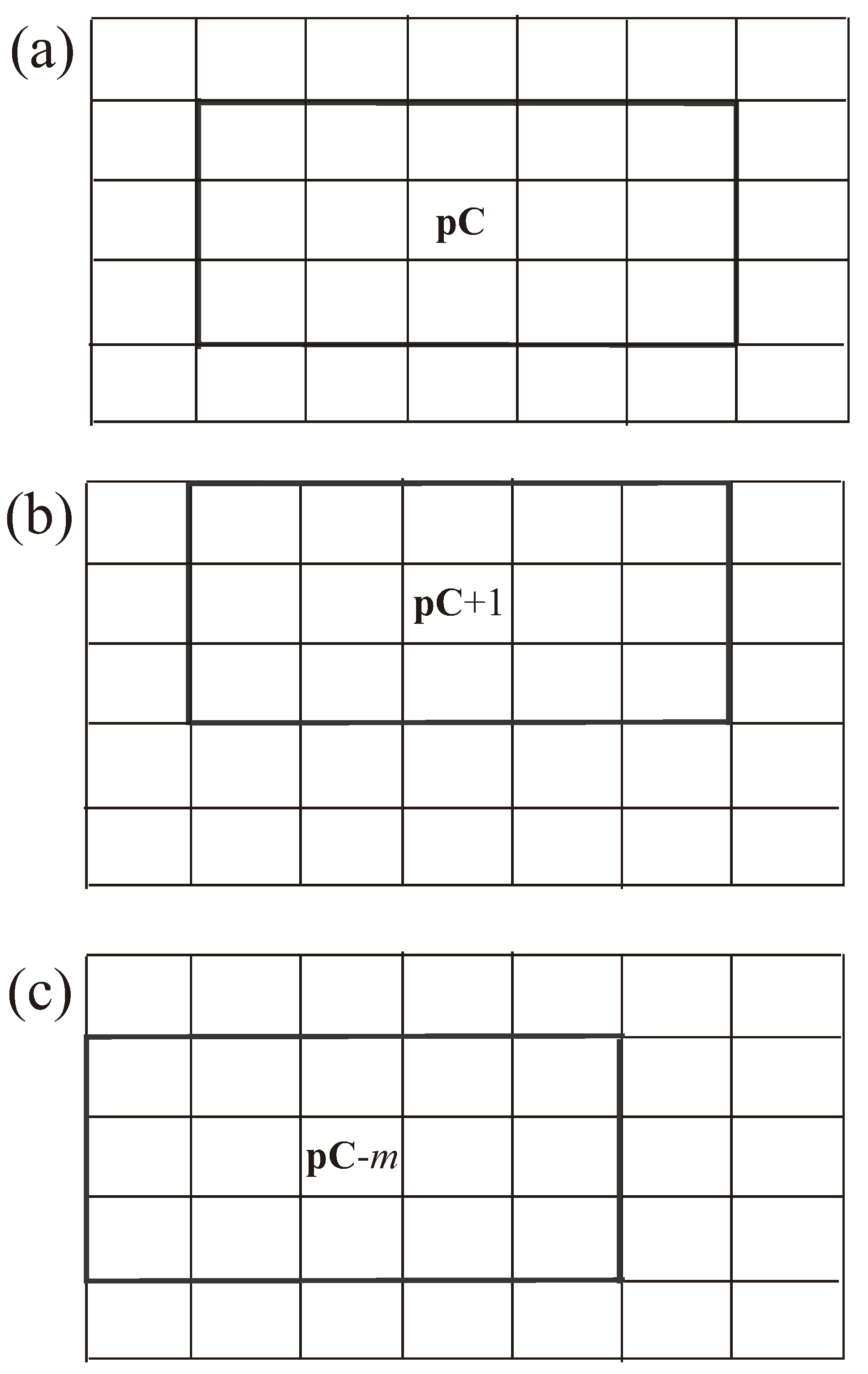
Using one-dimensional array of indices, it is possible to specify a subset of cells of mesh (Figure 1). For example, denoting by $\mathbf{pC}$ the vector (set) of indices of all internal cells (Figure 1a), subsets of cells that are above (Figure 1b) or below a current layer of cells are addressed. To address neighboring cells, it is necessary to add or subtract one from all components of the vector $\mathbf{pC}$

$$\begin{array}{c}\hfill \mathbf{pU}=\mathbf{pC}+1,\mathbf{pD}=\mathbf{pC}-1.\end{array}$$

Using similar procedure, the index vectors for left and right cells of computational domain are defined

$$\begin{array}{c}\hfill \mathbf{pL}=\mathbf{pC}-m,\mathbf{pR}=\mathbf{pC}+m.\end{array}$$

The integer value m determines the number of cells in the column of computational domain.

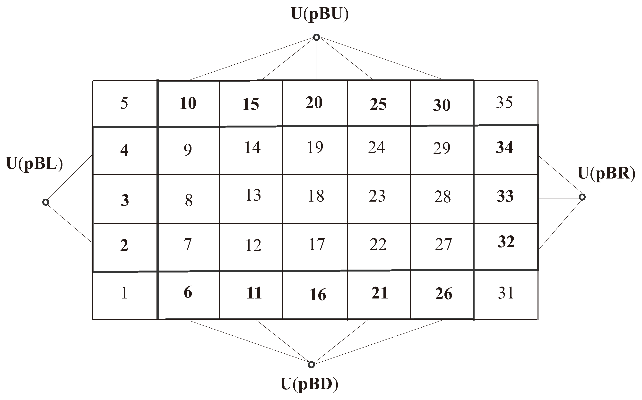
4.3. Addressing to Boundary Cells

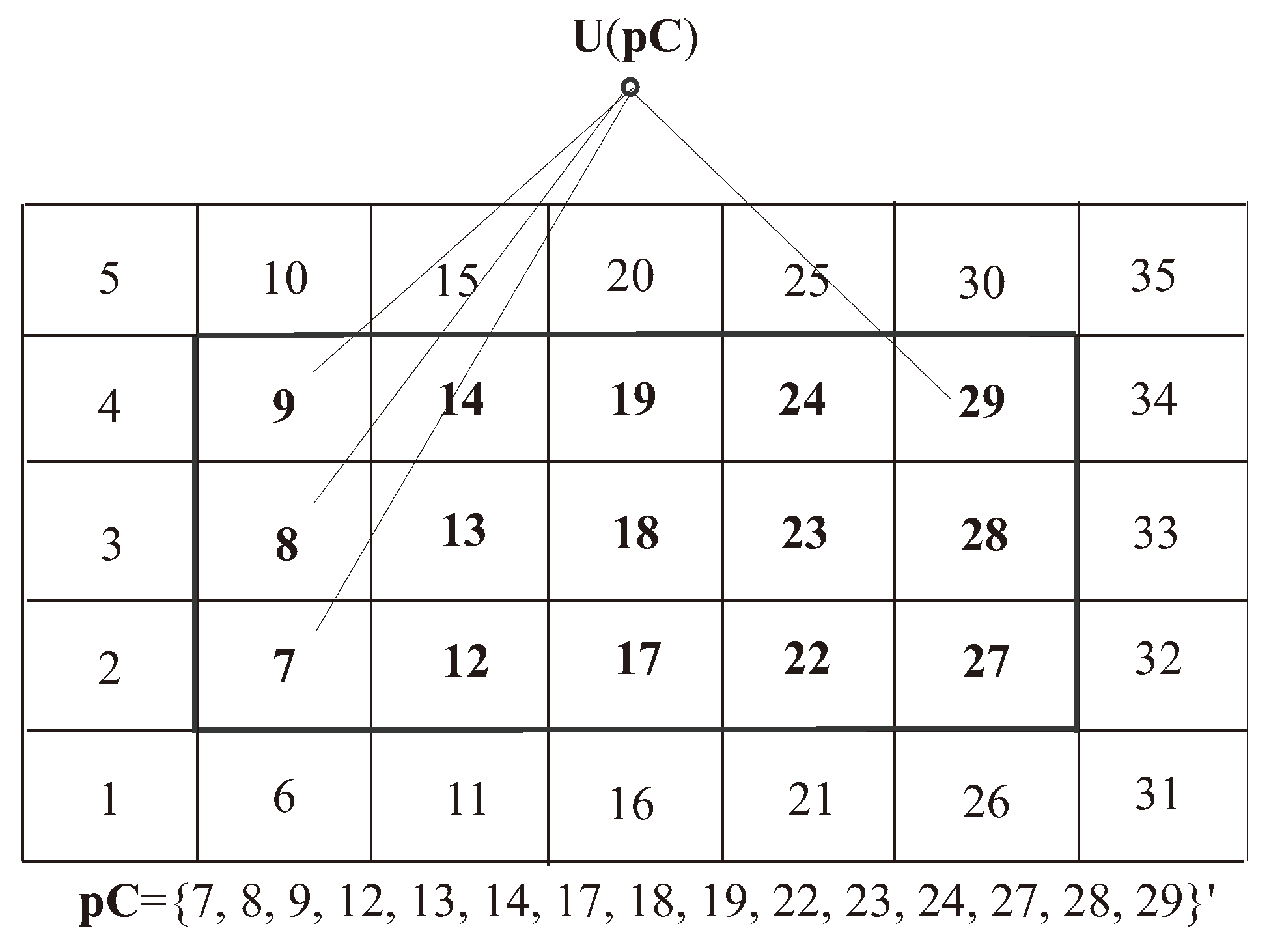
To set boundary conditions, ghost cells are used, forming with internal cells an extended computational domain. Internal cells are highlighted in bold in Figure 2, and addressing them is provided using the index vector $\mathbf{pC}$.

The method of addressing ghost cells is shown in Figure 3. For this purpose, index vectors $\mathbf{pBL}$, $\mathbf{pBU}$, $\mathbf{pBR}$, $\mathbf{pBD}$ are designed, corresponding to left, upper, right, and lower boundaries of computational domain. The method of their design is similar to index vectors of internal cells (corner cells are ignored).

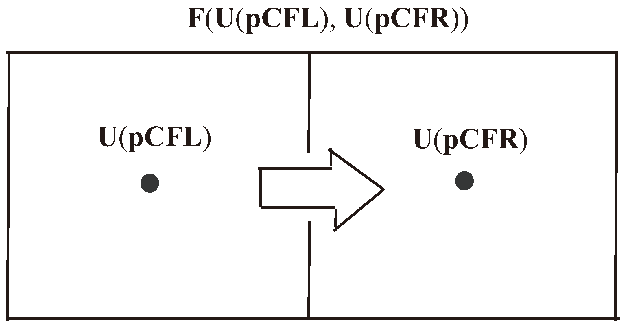
4.4. Flux Computation

The face separating two neighboring cells is selected as the object to which the flux is assigned. Linking the flux to a face allows to avoid re-calculating it when implementing conservation laws for the control volume. The same flux value is involved in constructing balance relations for two neighboring cells (the flux entering a cell equals the flux leaving the neighboring cell), which ensures the conservativeness of the numerical scheme.

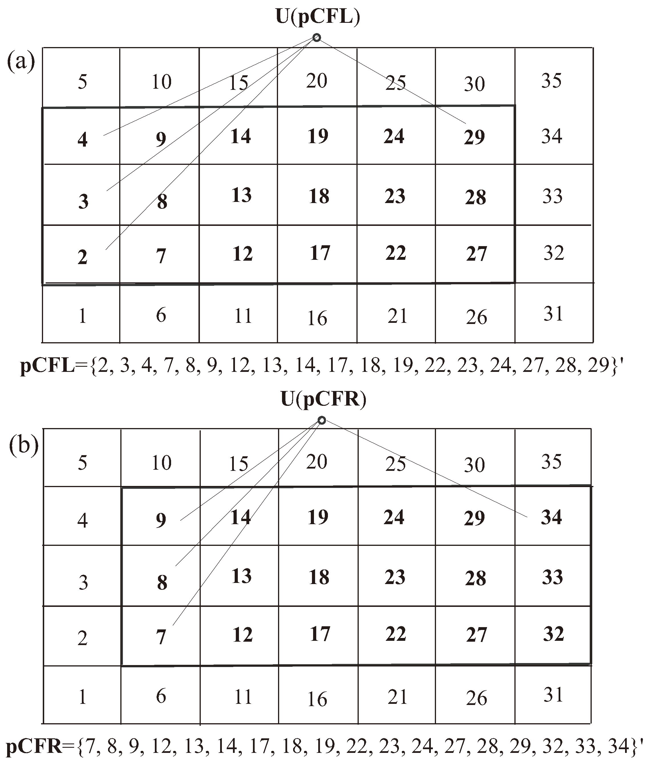
When introducing ghost cells, all control volumes located inside the computational domain have neighbors, and the calculation of fluxes for all faces is carried out using a single algorithm. To calculate fluxes, two sets of index vectors are formed (Figure 4). One of these vectors, $\mathbf{pCFL}$, defines the set of all cells located to the left of the face (Figure 4a), and another index vector, $\mathbf{pCFR}$, provides a wildcard addressing operation for the set of all right cells (Figure 4b). It is defined as follows

$$\begin{array}{c}\hfill \mathbf{pCFR}=\mathbf{pCFL}+m.\end{array}$$

The vector operation of numerical fluxes is provided by

$$\begin{array}{c}\hfill \mathbf{F}\left(\mathbf{pC}\right)=\mathbf{F}\left(\mathbf{U}\right(\mathbf{pCFL}),\mathbf{U}(\mathbf{pCFR}\left)\right).\end{array}$$

(3)

The sequence of calculations written in ordinary index expressions has the form

$$\begin{array}{c}\hfill {\mathbf{F}}_{i+1/2,j}=\mathbf{F}({\mathbf{U}}_{i+1,j},{\mathbf{U}}_{i,j}).\end{array}$$

(4)

Indices i and j refer to the center of the cell, and the index $i+1/2$ corresponds to the face separating cells with indices i and $i+1$.

There is a difference between expressions (3) and (4). While relation (3) defines the entire set of threads, relation (4) requires a double round of calculations on indices i and j. The advantages of the expression-based approach (3) are manifested when using computing environments that allow the execution of vectorized operations.

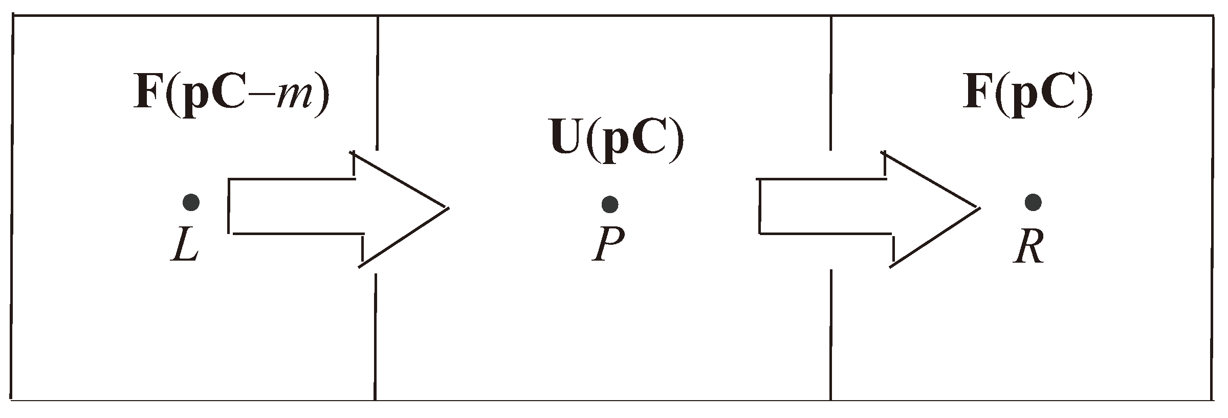
Since the flux is assigned to the cell face, and flow quantities are assigned to cell center (Figure 5), it is necessary to determine the correspondence of index expressions for calculating the fluxes with the indices that define the cells of the computational domain. Even though a flux contains fewer elements than an extended set of cells, it makes sense to store it in a structure of the same size (although a number of elements are not used, but addressing convenience and clarity prevail over memory-saving considerations).

An index vector is designed to determine the set of fluxes through the cell faces using a layout shown in Figure 6.

With this data organization, vectorized balance relationships are written for each cell of computational domain. Addressing fluxes through a set of cell edges is shown in Figure 7. For all computational cells defined by the index vector $\mathbf{pC}$, fluxes through their left faces are determined by the index vector $\mathbf{pC}-m$, and fluxes through the right faces are determined by the index vector $\mathbf{pC}$. The value m represents the number of cells in the extended cell area column and determines the shift from a two-dimensional matrix structure to a linear arrangement of elements.

5. Discretization of Derivatives

Consider a finite-volume discretization of the derivative of a mesh function $\mathbf{U}$ defined on a sequential set of N equally spaced nodes. This dataset is represented using a linear array containing N elements.

To calculate the derivative, the function y = diff(x,n) is defined, which returns finite difference of order n that satisfies the recurrent relation diff(x,n) = diff(x,n-1). If x is one-dimensional array

x = [x(1) x(2) ... x(n)],

then diff(x) is a vector of finite differences between neighboring elements

diff(x) = [x(2)-x(1) x(3)-x(2) ... x(n)-x(n-1)].

The number of elements of vector x is one less than the number of elements of vector diff(x). The derivative approximation of order n is diff(y,n)./diff(x,n), where “./” operation denotes element-wise division of vectors.

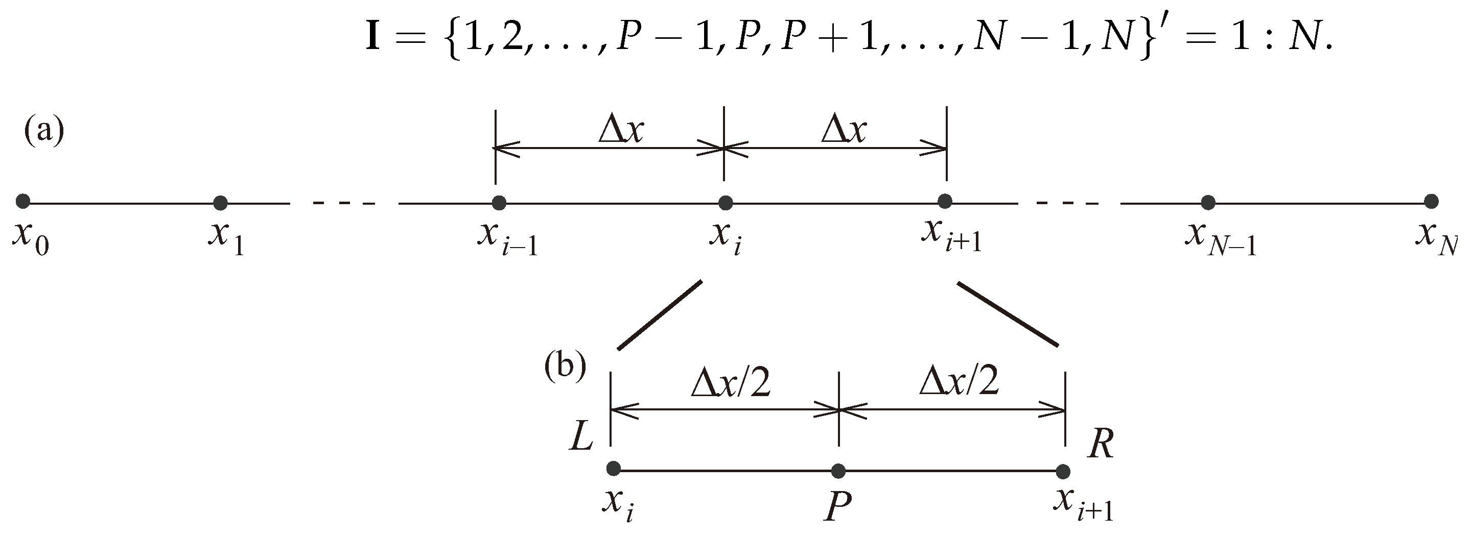
The derivative is calculated in another way, using the method of addressing mesh data structures. The integration interval $x_0⩽x⩽x_N$ is divided into N equal segments, and denote the length of each of them as $\Delta x=x_i-x_{i-1}$ (Figure 8a). A number of all intervals varies from 1 to $N-1$. An array of indices $\mathbf{I}$, in which the sequential increase in indices corresponds to the order of its elements, is

$$\begin{array}{c}\hfill \mathbf{I}={\left\{1,2,\dots ,P-1,P,P+1,\dots ,N-1,N\right\}}^{\prime }=1:N.\end{array}$$

The finite-difference template is shown in Figure 8b, where P is the midpoint of each segment, and the left and right boundaries of the interval are L and R, respectively (there are $N-1$ points P, L, and R in total). The arrays of indices for the left and right elements of mesh structure are introduced

$$\begin{array}{cc}\hfill & \mathbf{L}={\left\{1,2,\dots ,P-1,P,P+1,\dots ,N-2,N-1\right\}}^{\prime }=1:N-1;\hfill \\ \hfill & \mathbf{R}={\left\{2,3,\dots ,P-1,P,P+1,\dots ,N-1,N\right\}}^{\prime }=2:N.\hfill \end{array}$$

The vector subtraction operation is defined as

$$\begin{array}{c}\hfill \Delta \mathbf{U}=\mathbf{U}\left(\mathbf{R}\right)-\mathbf{U}\left(\mathbf{L}\right),\end{array}$$

where

$$\begin{array}{c}\hfill \left(\begin{array}{c}\Delta \mathbf{U}\left(1\right)\\ \Delta \mathbf{U}\left(2\right)\\ ⋮\\ \Delta \mathbf{U}(N-1)\end{array}\right)=\left(\begin{array}{c}\mathbf{U}\left(\mathbf{R}\right(1\left)\right)-\mathbf{U}\left(\mathbf{L}\right(1\left)\right)\\ \mathbf{U}\left(\mathbf{R}\right(2\left)\right)-\mathbf{U}\left(\mathbf{L}\right(2\left)\right)\\ ⋮\\ \mathbf{U}\left(\mathbf{R}\right(N-1\left)\right)-\mathbf{U}\left(\mathbf{L}\right(N-1\left)\right)\end{array}\right).\end{array}$$

Then, the formula for vectorized calculation of derivative has the form

$$\begin{array}{c}\hfill \frac{d\mathbf{U}\left(x\right)}{dx}=\frac{\mathbf{U}\left(\mathbf{R}\right)-\mathbf{U}\left(\mathbf{L}\right)}{\Delta x}+O(\Delta x^2).\end{array}$$

In a pseudo programming language that supports vectorized operations, the algorithm of derivative calculation is represented as the following sequence of steps.

 % indexes of intervals and boundary nodes

 iI=1:N-1; iL=iI; iR=iI+1;

 % mesh step

 dx=1/(N-1);

 % derivative y’(x)

 yp=(y(iR)-y(iL))/dx;

The presented method of addressing mesh data structures underlies the calculation of derivatives of mesh functions and the construction of vectorized algorithms for solving boundary value problems.

For the left and right boundaries, index vectors ${\mathit{I}}_L$ and ${\mathit{I}}_R$ are introduced, having dimension M, whose components are equal to 1 if the left/right boundary condition is specified for the component k of the solution vector, and 0 if there is no left/right boundary condition for the k component of the solution vector.

Two vectors $\mathit{L}$ and $\mathit{R}$ are formed. Their components contain, at the places determined by the index vectors ${\mathit{I}}_L$ and ${\mathit{I}}_R$, left and right boundary values, respectively, and the remaining components have undefined (arbitrary) values. Arbitrarily specified components of the vectors $\mathit{L}$ and $\mathit{R}$ do not take part in the calculations. Two integer numbers, $M_L$ and $M_R$, equal to the number of left and right boundary conditions (obviously, $M_L+M_R=M$), are introduced.

6. Boundary Value Problem

A system of ordinary differential equations of order M, resolved with respect to derivatives, is considered

$$\begin{array}{c}\hfill \frac{d\mathit{U}}{dx}+F\mathit{U}=\mathit{H},\end{array}$$

(5)

where $\mathit{U}$ is column vector of flow quantities, F is matrix of coefficients, $\mathit{H}$ is column vector of right-hand sides. To correctly solve a system of Equation (5), it is necessary that the number of boundary conditions be equal to the order of the system. In the general case, the boundary conditions between the initial $x_0$ and final $x_N$ nodes of the integration interval are distributed in an arbitrary ratio.

A vector of physical variables ${\mathit{U}}_i$ is assigned to each node of the computational domain $x_i$ ($i=0,\dots ,N$). Vectors ${\mathit{U}}_0$ and ${\mathit{U}}_N$, corresponding to the beginning and end of the integration interval, contain left and right boundary values.

For each point P, Equation (5) is written in discrete form

$$\begin{array}{c}\hfill \frac{{\mathit{U}}_R-{\mathit{U}}_L}{\Delta x}+F_P{\mathit{U}}_P={\mathit{H}}_P.\end{array}$$

(6)

The matrix of coefficients $F_P$ and the vector of right-hand side ${\mathit{H}}_P$ corresponding to node P as the half-sum of values related to points L and R are found as

$$\begin{array}{c}\hfill F_P{\mathit{U}}_P=\frac{1}{2}\left(F_L{\mathit{U}}_L+F_R{\mathit{U}}_R\right),{\mathit{H}}_P=\frac{1}{2}\left({\mathit{H}}_L+{\mathit{H}}_R\right).\end{array}$$

Substitution into Equation (6) provides

$$\begin{array}{c}\hfill {\mathit{U}}_R-{\mathit{U}}_L+\frac{\Delta x}{2}\left(F_L{\mathit{U}}_L+F_R{\mathit{U}}_R\right)=\frac{\Delta x}{2}\left({\mathit{H}}_L+{\mathit{H}}_R\right).\end{array}$$

(7)

To linearize the relationship (7), the frozen coefficient method is used.

7. Vectors of Computational Variables

Vectors ${\mathit{U}}_0$ and ${\mathit{U}}_N$, at some generally arbitrary places, contain quantities corresponding to the boundary conditions, which makes it difficult to formalize the computational procedure with vectors of physical variables.

Vectors of computational variables ${\mathit{W}}_i$ are introduced (their number is one less than physical vectors ${\mathit{U}}_i$). They contain only unknowns. Each computational vector ${\mathit{W}}_i$ contains part of the unknowns from the vector ${\mathit{U}}_{i-1}$ and part of the unknowns from the vector ${\mathit{U}}_i$. Obviously, any component of vectors ${\mathit{U}}_i$ is included in the set of vectors ${\mathit{W}}_i$ at most once. In this case, the known components of vectors ${\mathit{U}}_0$ and ${\mathit{U}}_N$ corresponding to boundary conditions are not included in vectors ${\mathit{W}}_i$.

The common scheme for constructing computational vectors ${\mathit{W}}_i$ is considered. The construction with the vector ${\mathit{W}}_N$ is the first step. The components of the vector ${\mathit{U}}_N$ that do not correspond to boundary conditions are transferred to the vector ${\mathit{W}}_N$ to the same places. The components remaining in the vector ${\mathit{W}}_N$ are filled with the components of the vector ${\mathit{U}}_{N-1}$ from the same positions. Formally, this procedure is written using the index vector ${\mathit{I}}_R$

$$\begin{array}{c}\hfill {\mathit{W}}_N^j=\left(1-{\mathit{I}}_R^j\right){\mathit{U}}_N^j+{\mathit{I}}_R^j{\mathit{U}}_{N-1}^j.\end{array}$$

(8)

Moving to the left from the right boundary (indices move from N to 1), the vector ${\mathit{W}}_i$ is represented as

$$\begin{array}{c}\hfill {\mathit{W}}_i^j=\left(1-{\mathit{I}}_R^j\right){\mathit{U}}_i^j+{\mathit{I}}_R^j{\mathit{U}}_{i-1}^j.\end{array}$$

(9)

The method for generating the vector ${\mathit{W}}_1$ differs from the others. The still unclaimed components of the vector ${\mathit{U}}_1$ take their positions, and the remaining places are filled with components of vector ${\mathit{U}}_0$ that do not correspond to the boundary conditions. To do this, these components are taken in increasing order of their indices and placed on the free places of vector ${\mathit{W}}_1$ in increasing order of indices of these places. The representation of vector ${\mathit{W}}_1$ has the form

$$\begin{array}{c}\hfill {\mathit{W}}_1^j=\left(1-{\mathit{I}}_R^j\right){\mathit{U}}_1^j+{\mathit{I}}_R^j{\mathit{U}}_{\ast }^j.\end{array}$$

(10)

The vector ${\mathit{U}}_{\ast }$ is obtained from the vector ${\mathit{U}}_0$ by rearranging the components according to the described principle. The formal representation of the vector ${\mathit{U}}_{\ast }$ is not essential for further presentation and is not provided here.

8. Transition Formulas

The vector of physical variables is expressed in terms of vectors of computational variables. Consider the agreement that the computational vector is formed taking into account the form of specifying the right boundary conditions

$$\begin{array}{c}\hfill {\mathit{U}}_i=T_L^i{\mathit{W}}_i+T_R^i{\mathit{W}}_{i+1},\end{array}$$

(11)

where $i=2,\dots ,N-1$. Relation (11) formalizes a simple shift in components, which is conducted in such a way that the components of computational vectors fall into place in the physical vectors.

The right permutation matrix $T_R$ contains the components of index vector ${\mathit{I}}_R$ on the main diagonal, and the remaining components of this matrix are zero

$$\begin{array}{c}\hfill T_R^i={\mathit{I}}_{R}E=\left(\begin{array}{cccc}{I}_R^1& 0& \cdots & 0\\ 0& I_R^2& \cdots & 0\\ ⋮& ⋮& \ddots & ⋮\\ 0& 0& \cdots & I_R^M\end{array}\right).\end{array}$$

The left permutation matrix $T_L$ contains zeros on the main diagonal where the corresponding components of index vector ${\mathit{I}}_R$ are equal to one, and ones otherwise, and the remaining components of this matrix are equal to zero

$$\begin{array}{c}\hfill T_L^i=E-T_R^i=\left(\begin{array}{cccc}1-I_R^1& 0& \cdots & 0\\ 0& 1-I_R^2& \cdots & 0\\ ⋮& ⋮& \ddots & ⋮\\ 0& 0& \cdots & 1-I_R^M\end{array}\right).\end{array}$$

The permutation matrices $T_L^i$ and $T_R^i$ are the same for all internal nodes of computational domain (for $i=1,\dots ,N-1$).

For the right boundary (for $i=N$), the representation of the vector of physical variables has the form

$$\begin{array}{c}\hfill {\mathit{U}}_N=T_L^N{\mathit{W}}_N+T_R^N\mathit{R}.\end{array}$$

(12)

The permutation matrices $T_L^N$ and $T_R^N$ remain the same as at the internal nodes.

The representation of vector of physical variables on the left boundary (at $i=0$) has a special form. To form the corresponding expression, several auxiliary matrix objects are introduced. Note that a square matrix having a single non-zero element equal to 1 in row l and in column k, when multiplied by a column vector, moves the element of vector k to position l. The representation of vector of physical variables at node $i=0$ is related to the form of computational vector at $i=1$. The structure of this relationship has the form

$$\begin{array}{c}\hfill {\mathit{U}}_0=T_L^0\mathit{L}+T_R^0{\mathit{W}}_1.\end{array}$$

(13)

The first term on the right side is the set of components of vector of variables that are determined by the boundary values at the left end of the interval. The second term represents those vector components that are determined during the solution process. The left permutation matrix has the form

$$\begin{array}{c}\hfill T_L^0=E-{\mathit{I}}_{L}E.\end{array}$$

The matrix $T_R^0$ provides the substitution of those variables that are not included in the boundary conditions and therefore are in the vector ${\mathit{W}}_1$.

To form the matrix $T_R^0$, the vector ${\mathit{W}}_1$ is filled with those components of the vector ${\mathit{U}}_1$ for which right boundary conditions are not specified (these components are formed in the same way as in other vectors). As a result, $M_L=M-M_R$ components are determined. To form the remaining $M_R$ components, the first zero element $I_L^j$ of the vector ${\mathit{I}}_L$ and the first non-zero element $I_R^k$ of vector ${\mathit{I}}_R$ are found. The pair of indices $(j,k)$ determines the transition of an element from ${\mathit{U}}_0$ to ${\mathit{W}}_1$. Then, the next pair of indices is determined and the process is repeated. The constructed set of $M_R$ pairs of indices allows to form a matrix $T_R^0$, which contains units in places indicated by pairs of indices (the first number of the pair indicates the row, and the second number of the pair indicates the column). Its remaining elements are equal to zero. The described procedure allows to connect the physical and computational vectors at node $i=0$ by a matrix relation.

9. Numerical Scheme

In the computational variables, the difference scheme for Equation (5) takes the form

$$\begin{array}{c}\hfill {\mathit{U}}_i-{\mathit{U}}_{i-1}+\frac{\Delta x}{2}\left(F_{i-1}{\mathit{U}}_{i-1}+F_i{\mathit{U}}_i\right)=\frac{\Delta x}{2}\left({\mathit{H}}_{i-1}+{\mathit{H}}_i\right).\end{array}$$

(14)

Considering the representation of vector of physical variables through the vector of computational variables, substitution into Equation (14) provides

$$\begin{array}{cc}\hfill & \left(-T_L^{i-1}+\frac{\Delta x}{2}{F}_{i-1}{T}_L^{i-1}\right){\mathit{W}}_{i-1}+\hfill \\ \hfill & \left[T_L^i-T_R^{i-1}+\frac{\Delta x}{2}\left(F_{i-1}{T}_R^{i-1}+F_i{T}_L^i\right)\right]{\mathit{W}}_i+\hfill \\ \hfill & +\left(T_i^R+\frac{\Delta x}{2}{F}_i{T}_R^i\right){\mathit{W}}_{i+1}=\frac{\Delta x}{2}\left({\mathit{H}}_{i-1}+{\mathit{H}}_i\right).\hfill \end{array}$$

(15)

In matrix form, the system of difference equations has the form

$$\begin{array}{c}\hfill A\mathit{U}=\mathit{B},\end{array}$$

(16)

where A is square matrix of coefficients of $MN\times MN$, $\mathit{U}$ and $\mathit{B}$ is column vector of unknowns and column vector of right-hand sides of $M\times N$. To solve a system of Equation (16), one of the methods for solving systems of linear equations is used, in particular, the traditional block Thompson method.

Relation (15) is written as

$$\begin{array}{c}\hfill A_i{\mathit{W}}_{i-1}+B_i{\mathit{W}}_i+C_i{\mathit{W}}_{i+1}={\mathit{D}}_i.\end{array}$$

(17)

Here,

$$\begin{array}{cc}\hfill & A_i=-T_L^{i-1}+\frac{\Delta x}{2}{A}_{i-1}{T}_L^{i-1};\hfill \\ \hfill & B_i=T_L^i-T_R^{i-1}+\frac{\Delta x}{2}\left(A_{i-1}{T}_R^{i-1}+A_i{T}_L^i\right);\hfill \\ \hfill & C_i=T_i^R+\frac{\Delta x}{2}{A}_i{T}_R^i;\hfill \\ \hfill & {\mathit{D}}_i=\frac{\Delta x}{2}\left({\mathit{B}}_{i-1}+{\mathit{B}}_i\right).\hfill \end{array}$$

Vectors ${\mathit{W}}_0$ and ${\mathit{W}}_{N+1}$ are taken to be vectors $\mathit{L}$ and $\mathit{R}$, respectively. For $i=1$ and $i=N$

$$\begin{array}{cc}\hfill & B_1{\mathit{W}}_1+C_1{\mathit{W}}_2={\mathit{D}}_1-A_1\mathit{L};\hfill \\ \hfill & A_N{\mathit{W}}_{N-1}+B_N{\mathit{W}}_N={\mathit{D}}_N-C_N\mathit{R}.\hfill \end{array}$$

The running relations are constructed according to the following dependence

$$\begin{array}{c}\hfill {\mathit{W}}_{i-1}=K_{i-1}{\mathit{W}}_i+{\mathit{P}}_{i-1}.\end{array}$$

Substitution leads to equation

$$\begin{array}{c}\hfill {\mathit{W}}_i=-{\left(A_i{K}_{i-1}+B_i\right)}^{-1}{C}_i{\mathit{W}}_{i+1}+{\left(A_i{K}_{i-1}+B_i\right)}^{-1}\left({\mathit{D}}_i-A_i{\mathit{P}}_{i-1}\right).\end{array}$$

As a result, the representations for $K_i$ and ${\mathit{P}}_i$ for $i>1$ have the form

$$\begin{array}{cc}\hfill & K_i=-{\left(A_i{K}_{i-1}+B_i\right)}^{-1}{C}_i;\hfill \\ \hfill & {\mathit{P}}_i={\left(A_i{K}_{i-1}+B_i\right)}^{-1}\left({\mathit{D}}_i-A_i{\mathit{P}}_{i-1}\right).\hfill \end{array}$$

The matrix $K_1$ and the vector ${\mathit{P}}_1$ are calculated using the relations

$$\begin{array}{cc}\hfill & K_1=-B_i^{-1}{C}_i;\hfill \\ \hfill & {\mathit{P}}_1=B_i^{-1}\left({\mathit{D}}_i-A_i\mathit{L}\right).\hfill \end{array}$$

The vector ${\mathit{W}}_N$ is found by the formula (forward step)

$$\begin{array}{c}\hfill {\mathit{W}}_N={\left(A_N{K}_{N-1}+B_N\right)}^{-1}\left({\mathit{D}}_N-C_N\mathit{R}-A_N{\mathit{P}}_{N-1}\right).\end{array}$$

Using the found values of the sweep coefficients, the following vector values are calculated, moving along the computational domain from left to right (reverse step)

$$\begin{array}{c}\hfill {\mathit{W}}_i=K_i{\mathit{W}}_{i+1}+{\mathit{P}}_i.\end{array}$$

To fill the physical vectors, transition formulas are used, described by the relations (11)–(13).

10. Results and Discussion

Vectorized algorithms are applied to solving benchmark CFD problems. The benchmark problems allow to validate the reconstruction procedure for the presence of phase errors, the occurrence of non-physical oscillations, and smoothing of the solution in the region of sharp gradients. The problem of wave convection serves to validate the reconstruction step of the numerical algorithm, and the shock tube problem allows to validate the evolution step.

10.1. Wave Convection

Equation of wave convection is a simple model of convective vortex transport. When studying wave processes, the case when the initial data are a sinusoidal (or cosine) distribution is interesting. The linear transport equation transports such a wave without distortion, while difference schemes that implement this equation can distort the wave, changing its amplitude and shape. The wave convection equation (scalar transport equation) is written as [26,27]

$$\begin{array}{c}\hfill \frac{\partial u}{\partial t}+a\frac{\partial u}{\partial x}=0,\end{array}$$

(18)

where $a=\mathrm{const}$. The initial condition includes Gaussian wave, square wave, triangular wave, or semi-elliptical wave. The boundary condition is

$$\begin{array}{c}\hfill u(x,0)=u_0\left(x\right).\end{array}$$

The general solution of transport equation for $a=\mathrm{const}$ is

$$\begin{array}{c}\hfill u=u_0(x-at).\end{array}$$

To validate the reconstruction step of the numerical algorithm, the initial condition for Equation (18) is specified in the form

$$\begin{array}{c}\hfill u(x,0)=exp\left(-x^2/16\right).\end{array}$$

The exact solution is

$$\begin{array}{c}\hfill \widehat{u}(x,t)=exp\left[-{(x-t)}^2/16\right].\end{array}$$

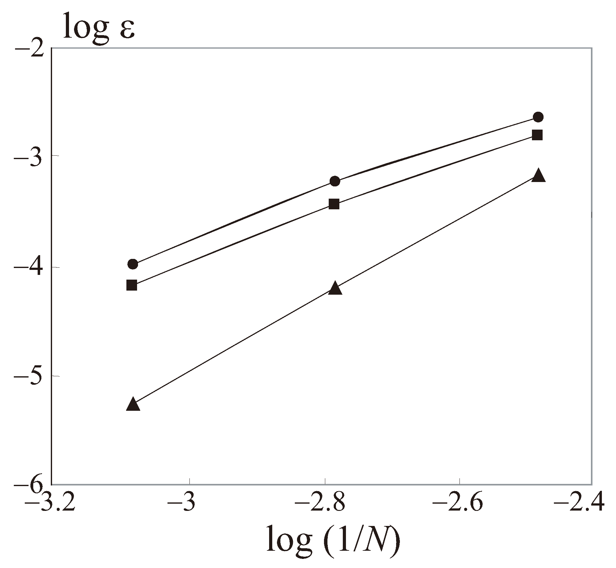
The numerical error is estimated as

$$\begin{array}{c}\hfill \delta =\frac{1}{N}{\left[{\displaystyle \sum _{i=1}^N}{\left(u_i-{\widehat{u}}_i\right)}^2\right]}^{1/2},\end{array}$$

where N is the number of mesh nodes.

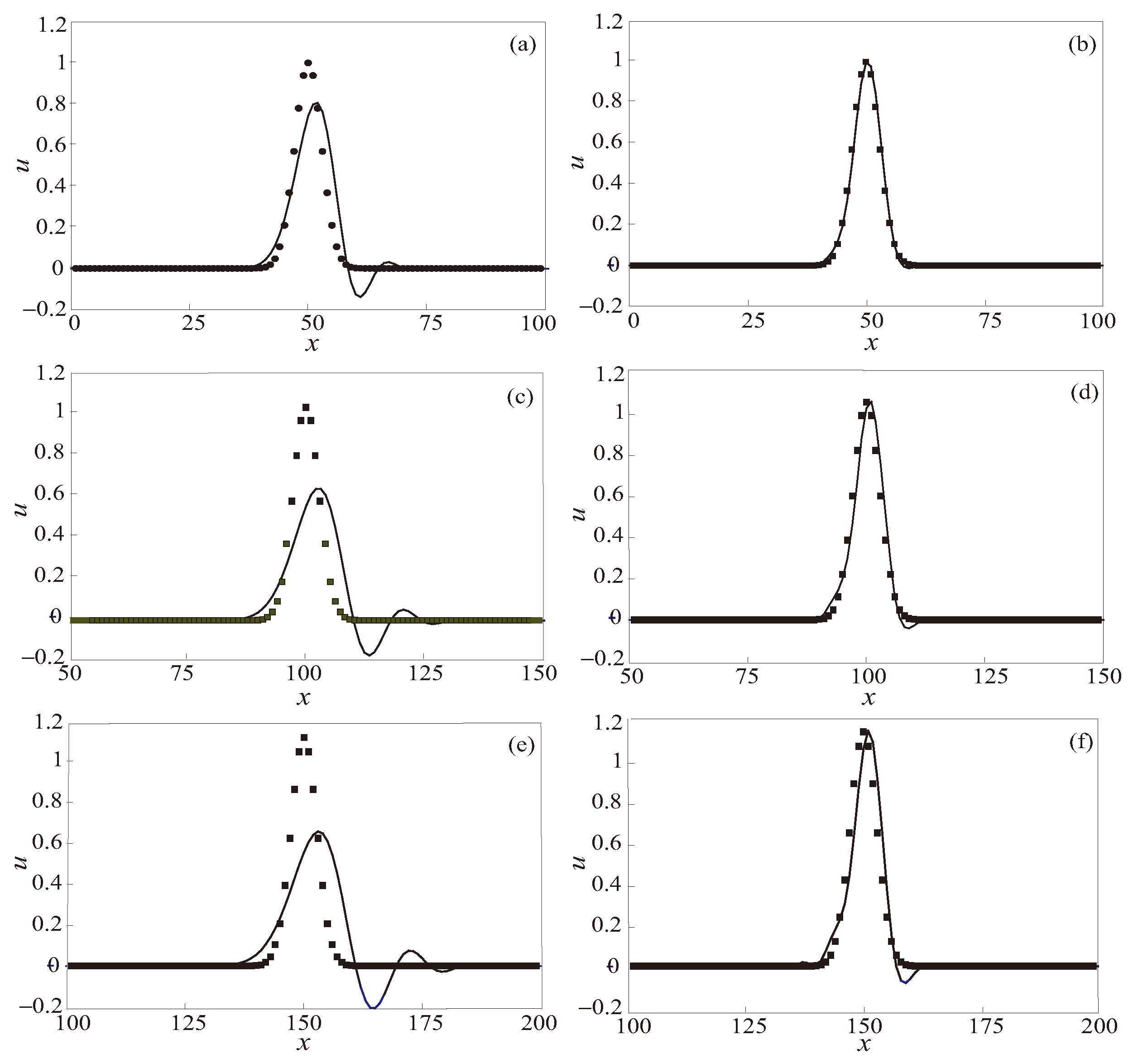
To discretize time derivatives, the three-step Runge–Kutta method is used, and UDS-3 scheme (upwind difference scheme) and STVD-4 and STVD-6 schemes (symmetric TVD scheme) are used to calculate fluxes.

The results of numerical calculations (solid line) are shown in Figure 9 in comparison with the exact solution (symbols ■). The results demonstrate that upwind scheme is too dissipative. It underestimates the maximum value of the unknown and leads to oscillations of the solution. Two numerical schemes of TVD type of second and third orders provide similar results. Increasing the order of numerical scheme makes it possible to achieve a higher accuracy with a smaller number of nodes but requires an increase in number of operations on each time layer (Figure 10).

10.2. Shock Tube

In a shock tube (Sod problem), two regions are occupied by a gas (a diaphragm is located at $x=0$). When diaphragm is broken, two gases interact with each other. The problem has exact solution. It consists of a shock or rarefaction wave travelling to the left region, a shock or rarefaction wave travelling to the right region, and contact discontinuity. A wave front of rarefaction wave represents a fan of flow characteristics.

The initial conditions correspond to two different solutions. Flow is subsonic in case 1, and flow is supersonic in case 2. Working substance is air; it is treated as ideal gas ($\gamma =1.4$).

In case 1, $\rho (x,0)=p(x,0)=2$ if $x⩽0$, and $\rho (x,0)=p(x,0)=1$ if $x>0$, $u(x,0)=0$. The mesh contains 100 cells (mesh step size is $\Delta x=1.0$). To reach a steady state, 100 time steps are applied (time step is $\Delta t=0.00058$). The Courant number is fixed at 0.59.

In case 2, $\rho (x,0)=p(x,0)=20$ if $x⩽0$, and $\rho (x,0)=p(x,0)=1$ if $x>0$, $u(x,0)=0$. The mesh contains 1000 cells (mesh step size is $\Delta x=0.1$). To reach a steady state, 100 time steps are applied (time step is $\Delta t=0.00012$). The Courant number is fized at 0.54.

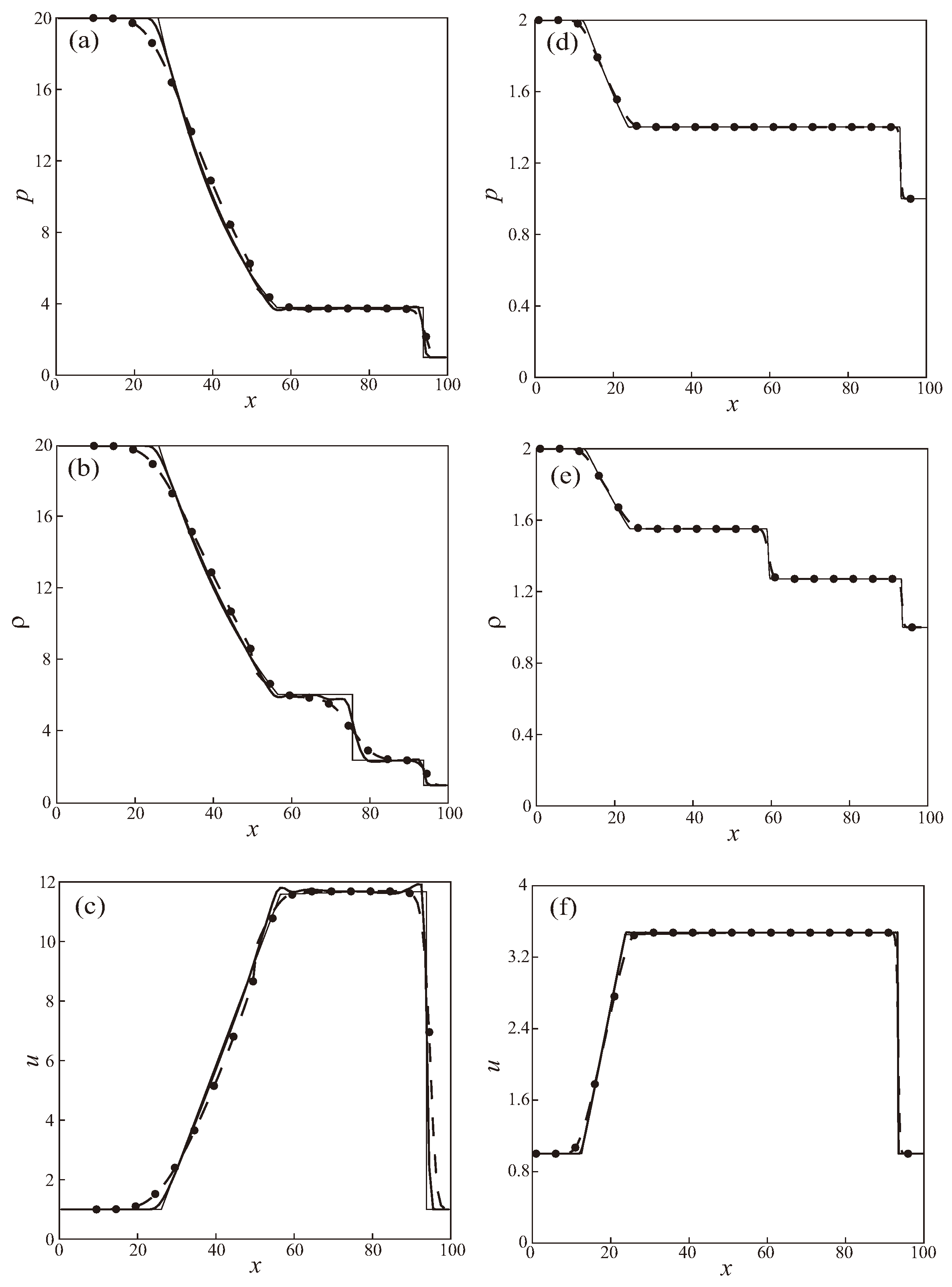
The distributions of flow quantities are shown in Figure 11. The graphs presented show numerical solutions in a short period of time when initial discontinuity starts to break and the largest disturbance from the exact Riemann solver is observed. Solid line corresponds to the exact solution of Riemann problem, dotted line corresponds to calculation with Godunov scheme, symbols • correspond to calculation with third-order numerical scheme, and circles correspond to calculation with the scheme using a piece-parabolic approximation of flow quantities in a control volume. In this case, Godunov scheme requires approximately 3.8 times more computational time than schemes with approximate solution of Riemann problem.

The solution of shock tube problem [28] has a monotonic density profile. Solution of Lax problem [29] provides verification of properties of numerical schemes. Various numerical schemes correctly predict horizontal parts of density distributions. The distributions computed with second-order scheme have a slight increase in density in 1–2 mesh cells to the right of contact discontinuity. The contact discontinuity is less smoothed in the numerical solutions computed with high-order accuracy schemes.

10.3. Flow around Expansion Corner

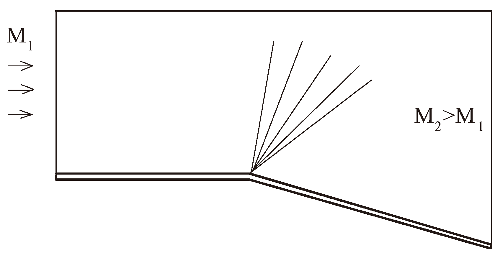
A Prandtl–Meyer flow around expansion corner is considered [30]. The corner angle is $\theta =6.{25}^{\circ }$. Corner point is located at $x=0$. Initial flow is parallel to lower wall (Figure 12). Total pressure and total temperature are fixed on inflow boundary ($p_0={10}^5$ Pa, $T_0=290$ K). Flow speed is 682 m/s, and Mach number is 2.0.

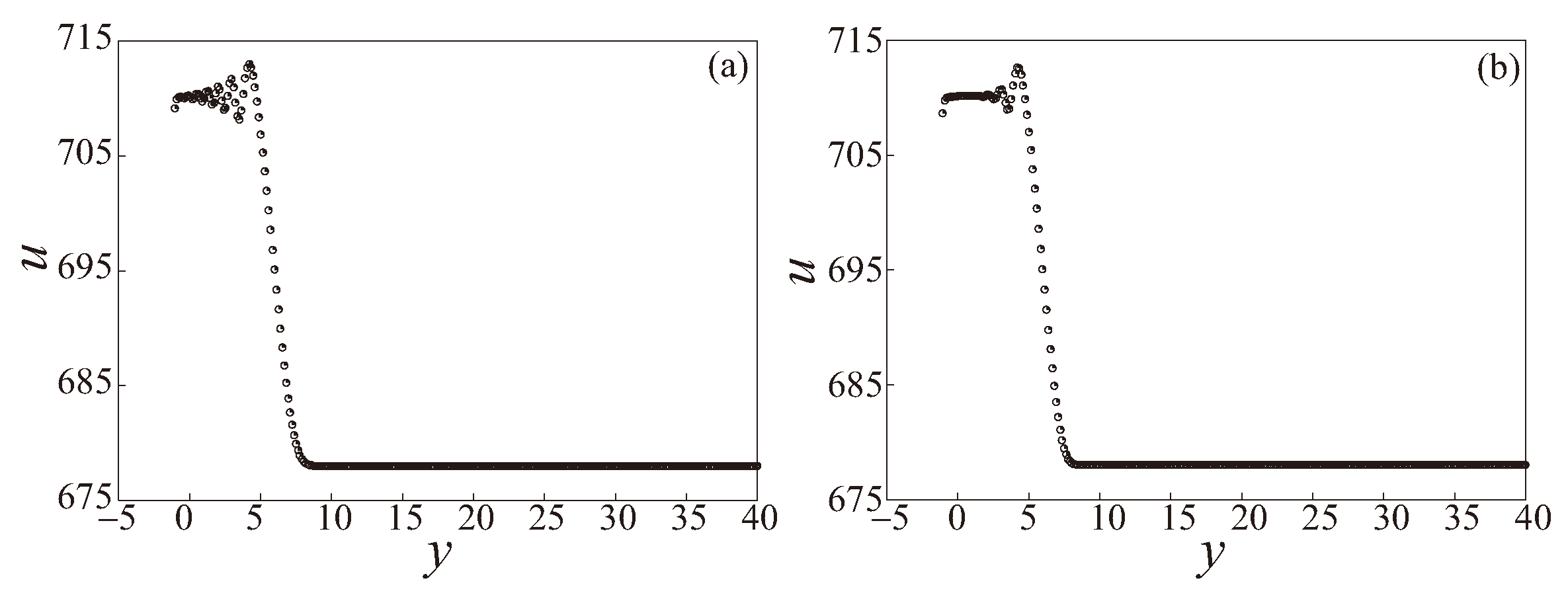
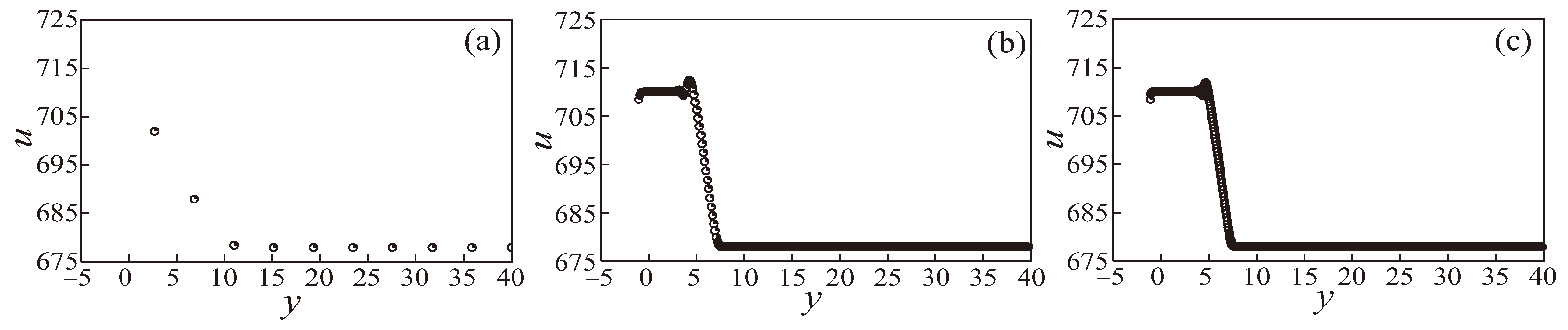
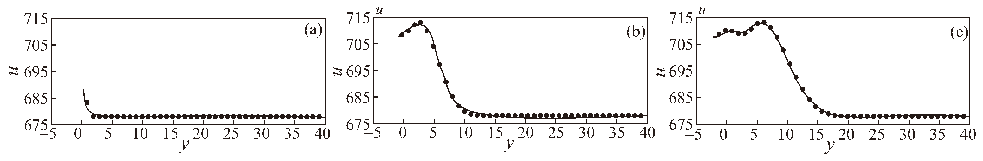
Solutions on a structured mesh with $65\times 41$ nodes (symbols •) and an unstructured mesh with 2600 nodes (solid line) are shown in Figure 13 for the fixed Courant number 0.54. Distributions of flow quantities for various Courant numbers are presented in Figure 14. The maximum velocity in the computational domain is about 711 m/s. If Courant number equals 0.1, oscillations of numerical solution occur, corresponding to the location of reversed flow. Distributions of velocity magnitude computed on different meshes are shown in Figure 15.

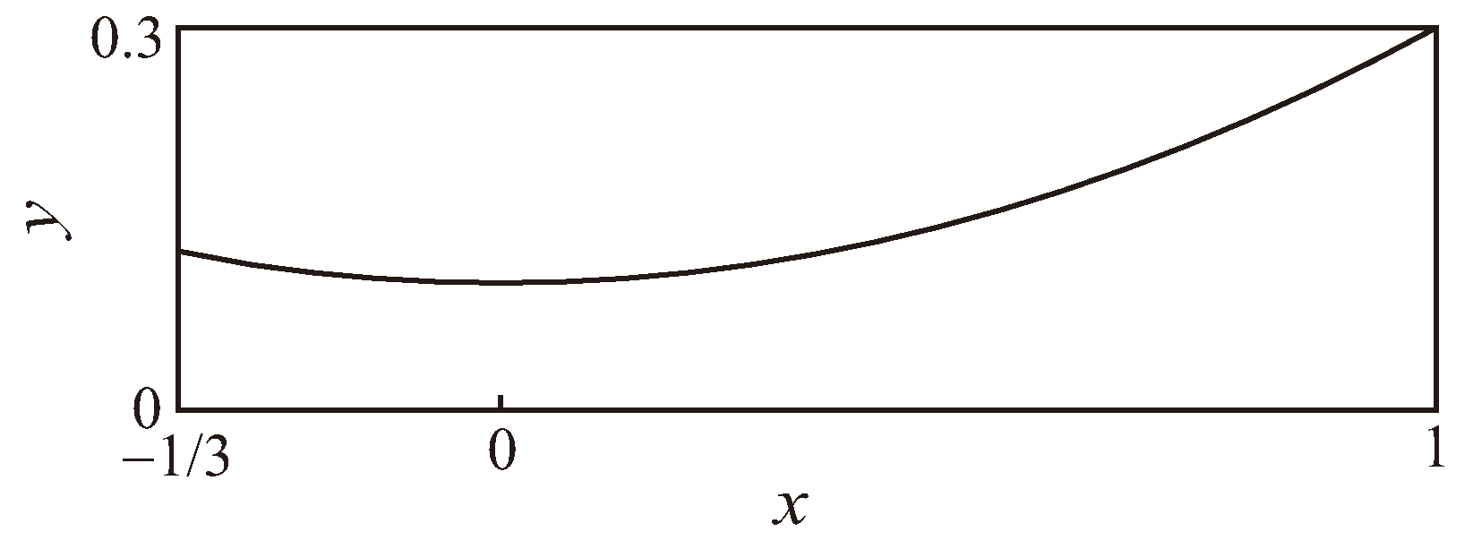
10.4. Nozzle Flow

An unsteady one-dimensional flow of inviscid compressible gas in a convergent-divergent nozzle is considered. Air ($\gamma =1.4$) is a working gas. The cross-sectional area of the nozzle varies as (Figure 16)

$$\begin{array}{c}\hfill S\left(x\right)=1+2x^2,\mathrm{where}-1/3⩽x⩽1.\end{array}$$

The numerical solution is compared with the exact solution in overexpanded and underexpanded flow regimes.

Total pressure and total temperature are fixed on inlet boundary ($p_0=p_{00}$, $T_0=T_{00}$). The third quantity is found from the characteristic relations. Specification of boundary conditions on outlet boundary depends on flow regime (flow speed), overexpanded or underexpanded. Flow regime on outlet boundary depends on nozzle pressure ratio

$$\begin{array}{c}\hfill \frac{p_{\infty }}{p_{00}}={\left(\frac{2}{\gamma +1}\right)}^{\frac{\gamma }{\gamma -1}}.\end{array}$$

A static pressure on outlet boundary equals atmospheric pressure ($p=p_{\infty }$) if outflow is subsonic. Overexpanded flow regime occurs if $p_{\infty }/p_{00}>0.528$ (pressure is restored to atmospheric pressure through a nozzle shock wave). No nozzle shock wave occurs if $p_{\infty }/p_{00}<0.528$ (the flow speed continuously increases in streamwise direction). Calculations are carried out on a mesh containing 35 cells, with a step of $\Delta x=0.038$. Initial conditions assume that $u=0$, $p_0=p_{00}$, $T_0=T_{00}$.

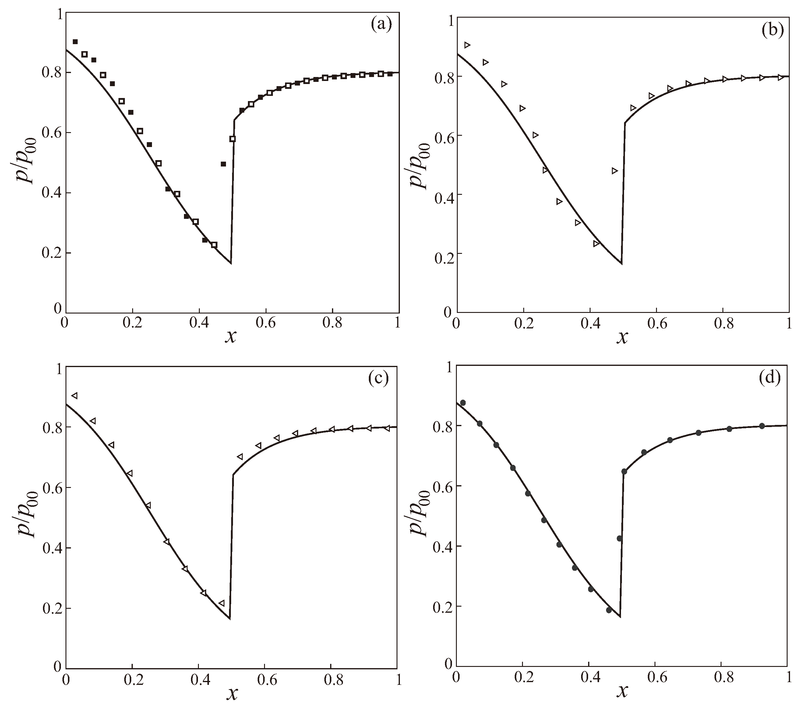
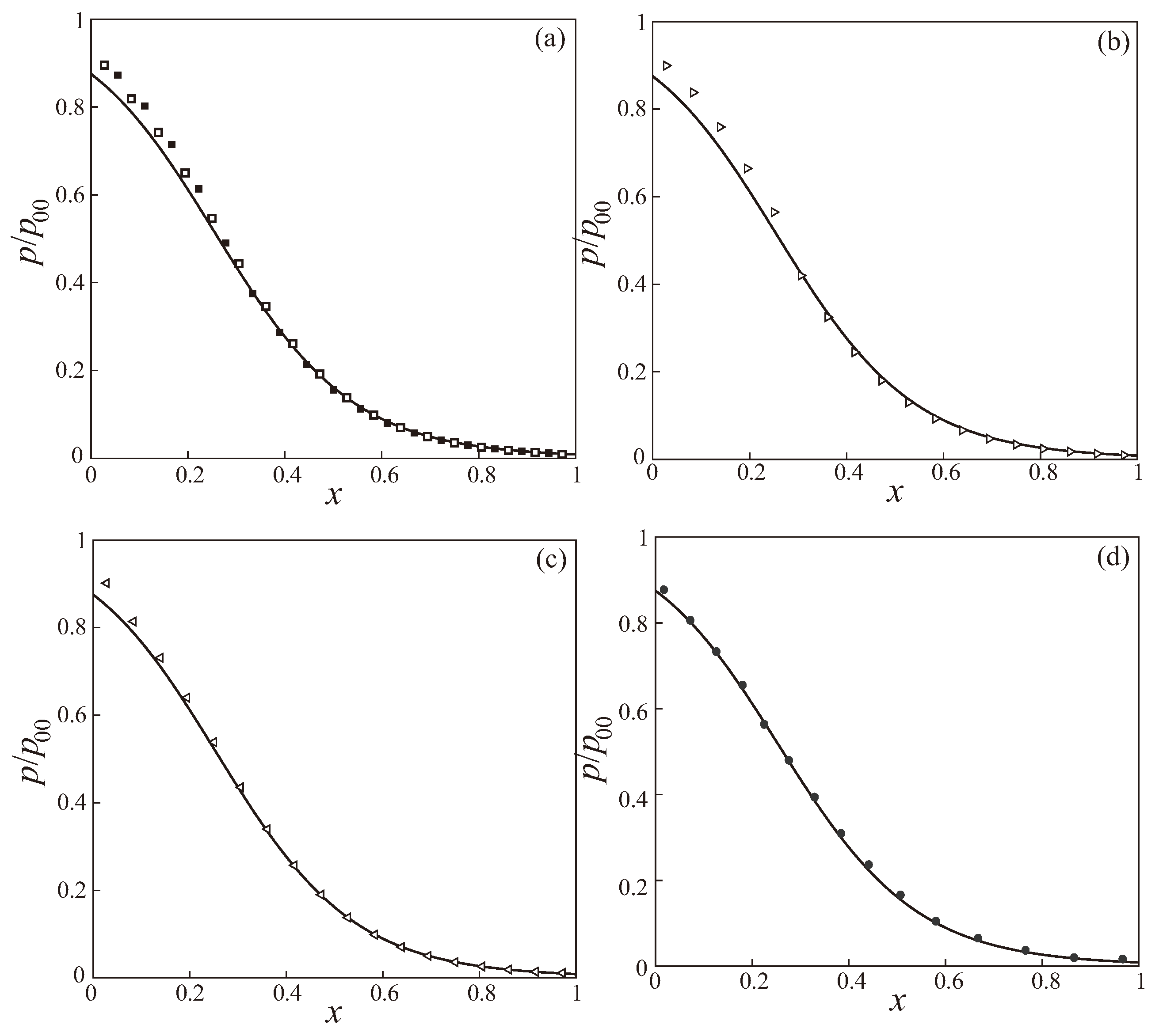
The results of numerical simulation, processed in the form of pressure dependencies on streamwise coordinates, are shown in Figure 17 (Courant number is 0.88) and Figure 18 (Courant number is 0.18). The symbols ■ and □ correspond to Godunov-type schemes of first and second orders (figure a), symbols ⊳ correspond to Roe scheme (figure b), symbols ⊲ correspond to TVD scheme of second order (figure c), and symbols • correspond to TVD scheme of third order (figure d). The computed results show that numerical schemes spread the discontinuity over 1–2 mesh cells, preserving the monotonic nature of numerical solution.

In the case of the presence of a nozzle shock wave (Figure 17), the third-order TVD numerical scheme provides results that are close to the exact solution. When using the Godunov scheme, it takes 0.0352 s of estimated time (fourteen time steps) to achieve a steady state; the Godunov scheme of second order takes 0.0348 s (eleven steps); the Roe scheme takes 0.02 s (five steps); and the TVD schemes of second and third orders take 0.021 s (four steps) and 0.023 s (four steps).

Numerical schemes provide similar results in overexpanded flow regimes. The Godunov scheme takes 0.0068 s (twelve time steps) to achieve a steady state; the Godunov scheme of second order takes 0.0082 s (sixteen steps); the Roe scheme takes 0.01 s (nineteen steps); and the TVD schemes of second and third orders take 0.007 s (thirteen steps) and 0.0072 s (eleven steps).

11. Conclusions

Using loops is a common and natural tendency when performing repetitive operations in programming. However, when working with a large number of iterations, such as millions or billions of rows, using loops can lead to poor performance and long run times. In these cases, implementing vectorization can greatly improve efficiency and avoid the frustration of waiting for slow processes to complete. Vectorized operations enable the use of efficient pre-compiled functions and mathematical operations on arrays and data sequences.

An approach to the construction and implementation of vectorized algorithms for solving CFD benchmark problems has been developed. The capabilities of the developed approach are demonstrated by solving a number of CFD problems. Speed is important because small differences in runtime can accumulate and become significant when repeated over many function calls. For example, an incremental 30 microseconds of overhead, when repeated over 1 million function calls, can result in 30 s of additional runtime.

The Riemann solver has a function that processes the right and left decay profiles of a discontinuity in the same way, with minor changes. Using a simple change in variables, which consisted of changing the sign of the velocity value, it was possible to merge the code for two subtrees. This allowed us to halve the volume of calculation code and reduce execution time by 45%.

The developed methods for vectorizing a complex software context can be used to optimize other computational problems. In particular, a library is being developed aimed at vectorizing arbitrary planar cycles, that is, cycles in which there are no interiteration dependencies.