Abstract
In this study, we develop new efficient parallel techniques for solving both distinct and multiple roots of nonlinear problems at the same time. The parallel techniques represent an innovative contribution to the discipline, with local convergence of the ninth order. Theoretical research shows the rapid convergence and effectiveness of the proposed parallel schemes. To assess the suggested scheme’s stability and consistency, we look at certain biomedical engineering applications, such as osteoporosis in Chinese women, blood rheology, and differential equations. Overall, detailed analyses of convergence behavior, memory utilization, computational time, and percentage computational efficiency show that the novel parallel techniques outperform the traditional methods. The proposed methods would be more suitable for large-scale computational problems in biomedical applications due to their advantages in memory efficiency, CPU time, and error reduction.
1. Introduction
Nonlinear equations have been used for practical problem-solving from the time of ancient civilizations such as Babylon and Egypt [1]. In ancient mathematics, they were fundamental to astronomy, land measuring, building, and the computation of areas, volumes, and geometric difficulties [2,3]. Methods for dealing with increasingly complex nonlinear equations arose with contributions from Greek and Arab mathematicians [4], resulting in advances in algebra [5,6].
In many branches of science and engineering today, nonlinear equations are still essential. They are employed in mechanical and biomedical engineering to simulate biological systems [7], including pharmacokinetics and enzyme kinetics [8], which forecast medication concentration over time [9]. Nonlinear models also help with medical imaging, specifically reconstruction methods used in CT and MRI scans [10]. For effective manufacturing, polynomials are used in chemical engineering to model material attributes, improve process conditions, and define reaction rates. In order to ensure structural integrity and performance efficiency, nonlinear equations in mechanical engineering help define stress–strain relationships, characterize aerodynamic features, and support mechanical design optimization [11,12]. Thus, nonlinear equations nevertheless serve as a link between cutting-edge scientific and engineering applications and old mathematical truths.
Nonlinear equations are important because they may be used to describe and predict complex systems precisely, which can lead to important advancements in a variety of engineering and scientific fields [13]. Recent advances in computing technologies, as well as the increasing complexity of current engineering issues, have highlighted the importance of efficient and accurate solutions to nonlinear equations. Designing cutting-edge technology in the fields of renewable energy, aerospace, and telecommunications requires these solutions.
Nonlinear equations are significant in biomedical engineering [14] because they represent complex systems and biological processes that are intrinsically nonlinear. They are crucial in modeling physiological dynamics such as blood flow in arteries [15], oxygen diffusion in tissues [16], and electrical activity in the heart and brain [17]. These equations are fundamental to the design of medical devices such as pacemakers, artificial organs, and prosthetics, guaranteeing that their functionalities are compatible with natural systems. Nonlinear models aid in the simulation of drug distribution and pharmacokinetics, allowing therapies to be optimized. They also simplify the study of biomechanics subjects including joint movement and tissue deformation [18]. Nonlinearities in biomedical engineering also replicate sickness progression, resulting in improvements in specific treatment and early detection. They are utilized in systems biology, which investigates the interactions between biological networks [19] and bioinformatics [20] using nonlinear equations to better data interpretation and simulations.
Despite its importance, solving nonlinear equations remains difficult due to their intrinsic complexity and extensive processing resources required for advanced numerical iterative methods to obtain approximate solutions; see, e.g., [21,22,23]. The underlying non-locality of these models, in which the derivative at a location is determined by the complete history of the function, makes them infamously difficult to solve both analytically and numerically.
The main contribution of this research work is the development and analysis of parallel schemes designed specifically for solving nonlinear equations in diverse biomedical engineering applications. Indeed, these strategies have been carefully tested against conventional methods for computational efficiency, convergence rate, and even CPU time. The results clearly demonstrate the practical benefits of our technique, demonstrating that it is likely to handle biological problems in a computationally more effective manner than direct approaches. In-depth examination of convergence behavior, memory consumption, computation time, and computational efficiency as a percentage shows that the new parallel approaches perform better than the current ones. Our findings demonstrate significant improvements in CPU time, memory efficiency, and error reduction, which makes the proposed approaches more suitable for complex computing problems in biomedical applications and demonstrates the field’s noval contribution. Consequently, the findings of this study represent a significant advancement in the field of numerical methods, specifically in biomedical engineering.
The rest of the study is structured as we develop and analyze the parallel method in Section 2. Section 3 discusses percentage computational convergence analysis using computational percentage efficiency, as well as certain biomedical engineering applications to examine for efficiency and stability in terms of parallel processing time and memory utilization. The paper concludes with the last section.
2. Parallel Computing Scheme Construction and Theoretical Convergence
Direct numerical methods, such as single-step methods [24,25], multi-step methods [26,27], and hybrid methods [28] as well as exact techniques [29] and analytical techniques [30,31] have several drawbacks to solving nonlinear equations,
such as high computational costs, stability problems, and sensitivity to small errors. These methods are versatile and often simple to implement, but they have numerous important disadvantages. While these methods converge quickly near initial guesses, they can diverge if the guess is far from the exact solution or the function is complex. They are time-consuming and computationally expensive since they rely on accurate estimates for each root and are sensitive to initial assumptions. Computational costs rise while evaluating the function and its derivative, particularly for complicated functions. Furthermore, distinguishing between actual and complicated roots might be difficult without adjustments. Parallel root-finding methods, in contrast, provide more stability, consistency, and global convergence than single root-finding methods. They can be implemented on parallel computer architectures using many processes to approximate all solutions to (1) simultaneously.
Among parallel numerical schemes, the Weierstrass–Durand–Kerner approach [32] is particularly attractive from a computational standpoint. This method is given by
where
is Weierstrass’ correction. Method (3) has local quadratic convergence. Nedzibov et al. [33] present the modified Weierstrass method,
also known as the inverse Weierstrass method, which has quadratic convergence. Inverse parallel techniques outperform classical simultaneous approaches because they efficiently handle nonlinear equations and use parallel processing to expedite convergence. It adjusts dynamically to the particular characteristics of the problem, cutting down on computation time and increasing accuracy. This approach is especially applicable in large-scale or complex systems when traditional methods may be too slow or ineffective. The inverse parallel scheme is presented by Shams et al. [34] as
Inverse Parallel Scheme (5) has local quadratic convergence.
In 1977, Ehrlich [35] introduced a convergent simultaneous method of the third order given by
where
Shams et al. [36] presented the fractional parallel approach with Convergence Order 2 for solving (6) as follows:
where The following parallel technique of convergence order four was developed by Nourien [36] as follows:
The Zhang et al. method [37] is
where Using as a correction in (9), Petkovic et al. [38] accelerated the convergence order from three to six:
where and .
Motivated by the previously mentioned technique, the main aim of this research work is to develop efficient parallel numerical techniques for simultaneously finding all solutions of (1) at one time. This research work’s primary contributions are as follows:
- Construction and theoretical convergence study of parallel numerical schemes.
- Calculate the percentage computational efficiency.
- Using relatively rough initial estimations to test the efficiency and consistency of the parallel schemes.
- Assessing the developed parallel scheme’s versatility and stability on random initial approximations for biomedical engineering applications.
- Computing memory usage and computation time in seconds while applying the techniques on parallel processors.
- Estimating the number of basic arithmetic operations, number of functions and their derivative evaluations, percentage convergence on each iteration steps using random and rough starting values.
The parallel schemes approach is a powerful iterative technique for simultaneously finding all the roots of a nonlinear equations. This approach has useful applications in a variety of technical domains and is well known for its effectiveness and stability, particularly when dealing with intricate roots. It aids in the design of stable systems in control engineering by locating transfer function poles. In signal processing, it helps with spectral analysis and filter construction. The technique is also utilized in biomedical engineering to solve nonlinear equations in order to analyze various problems and forms of biomedical treatment. Here, we consider the following scheme [39] for finding simple root of nonlinear equations as
where The order of convergence of (11) is five and satisfies the following error equations:
where and We consider
to be a nonlinear polynomial equations with with root Thus,
This offers
Therefore, replacing with we obtain (6). Using (3), and (14) in (11), we develop a new parallel scheme (BF[∗]) for simultaneously finding all roots of (1) as
where For multiple roots the method can be written as
where
The following theorem defines the local order of convergence for the inverse fractional scheme.
Theorem 1.
Let be simple roots of a nonlinear equation and assume that the initial distinct estimates are sufficiently close to the true roots. Then, the method achieves a convergence order of nine.
Proof.
We let and represent the errors in and , respectively. From the first step of , we have
Thus, assuming we have
In the second step, we obtain
leading to
where We assume and
Thus, and we have
This completes the proof. □
3. Computational Efficiency and Numerical Results
The computational efficiency of parallel numerical techniques is crucial in tackling nonlinear biomedical engineering applications where distinct and many solutions must be computed simultaneously. Efficient parallel numerical algorithms can handle a larger number of nonlinear biomedical applications with higher degrees of nonlinearity, lowering computational time and resource requirements, which is critical for applications that require rapid processing, such as real-time systems and large-scale scientific computations. The parallel technique, which was recently developed, can improve convergence rates while minimizing errors in finding complex roots. High computational efficiency guarantees that these techniques continue to be viable for systems with constrained resources as well as high-performance computing environments. All simulations were performed on MatLab R2016a with the following hardware configuration to ensure the reliability and consistency of the study findings:
- Processor: Intel(R) Core(TM) i7-8650U CPU @ 1.90 GHz (2.11 GHz);
- Installed RAM: 16.0 GB (15.8 GB usable);
- System Type: 64-bit operating system, x64-based processor;
- Operating System: Windows 11 Pro.
In domains such as physics, engineering, and data science, efficient schemes enable the interpretation and dependability of numerical results by lowering iteration counts and computational overhead, improving memory management, and accelerating convergence. These factors are critical for analyzing large systems and improving solution accuracy. The information in Table 1 and the percentage computational efficiency [40]
can be used to evaluate the efficiency of the newly developed parallel schemes compared to existing methods in the literature. The following numerical schemes of the convergence order are compared in terms of percent computational efficiency, consistency, and stability. In the Perkovic et al. [41] method,
where

Table 1.
Numerical results of parallel schemes for solving.
the Wang–Wu technique [42] combined with first step as a Newton method,
and the Farmer–Loizou-like techanique [43] combined with the Newton method at the first step.
where
where the number of division for all methods is the same, i.e., 2
Table 2 displays the percentage computing efficiency of the newly developed approach in comparison to the previous method. It is evident from Table 2 that there are fewer basic mathematical operations per iteration than with other approaches currently in use. In the next sections, the efficiency, stability, and consistency of the newly devised approach in comparison to the existing method for addressing biomedical engineering applications are demonstrated using the data provided in Table 2 and the following stopping criteria:
where is error or norm .
Table 2.
Percentage computational efficiency of parallel schemes.
In the experimental section, we compare our newly developed parallel techniques with existing algorithms to assess their performance in nonlinear biomedical engineering problems. Key variables such computational efficiency, convergence rate, memory utilization, and CPU time are the focus of the experiments. In contrast to existing parallel schemes in the literature, a few biomedical engineering applications are taken into consideration to evaluate the method’s generalizability and applicability. In order to provide a thorough study, the evaluation also includes error graphs and a comparison of percentage computational efficiency. Thus, it highlights the advantages of the proposed approach and provides a clear explanation of the experimental setup and context for the numerical outcomes using Algorithm 1.
| Algorithm 1 Parallel scheme for solving nonlinear equations |
|
3.1. Biomedical Engineering Application 1: Osteoporosis in Chinese Women
Osteoporosis is a major health concern for Chinese women [44] who are at higher risk due to genetic, nutritional, and lifestyle factors. Chinese women are more susceptible to fractures when their bone density declines with age, which can result in lower quality of life and disability. Discussing osteoporosis in this demographic is critical for increasing awareness and encouraging preventative actions, as early interventions such as nutrition, exercise, and medication can significantly lower risk. Addressing this issue also contributes to public health strategies focused at reducing the burden of osteoporosis on China’s aging populations. The osteoporosis designs are mathematically modeled, leading to the following nonlinear equations [45]:
where offers the following nonlinear equations as
Non-linear Equation (36) has the following exact roots, accurate up to ten decimal places:
To determine the pace at which the suggested shemes converge, we conduct a very rough initial approximation as
The numerical outcomes on these rough initial approximations are given in Table 3.
Table 3.
Numerical results of parallel schemes using (38).
Table 3 and Table 4 illustrate that, in terms of residual error at rough initial approximation, our technique relatively better approximates all biomedical solutions with greater decimal places of accuracy when employing the defined stopping criteria (34). Figure 1a–d graphically displays the residual error in relation to the number of iterations using (38) to approximate all roots of (36) simultaneously. However, Table 4 and Figure 2a–d provide the overall performance in terms of consistency and efficiency. Table 4 and Figure 2a–d show that our method outperforms existing methods PM NN in terms of iterations, basic arithmetic operations , memory usage, percentage convergence, and computer processing time (CPU time).
Table 4.
Consistency analysis using (38) as starting values.
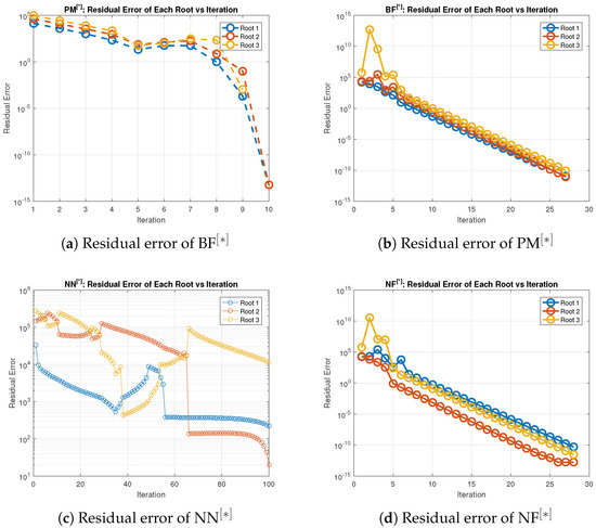
Figure 1.
(a–d) Error graph of the parallel schemes for solving (36).
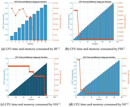
Figure 2.
(a–d) CPU time and memory consumed by parallel scheme for solving (36).
To check the global convergence on random initial generated vectors for the consistency and stability analysis of the scheme for solving biomedical engineering application, the outcomes are presented in Table 5, Table 6 and Table 7 and Figure 3a–d, respectively.
Table 5.
Iterations and percentage convergence on random initial values.
Table 6.
Memory and computational time in seconds.
Table 7.
Consistency analysis of the parallel schemes for solving (36).
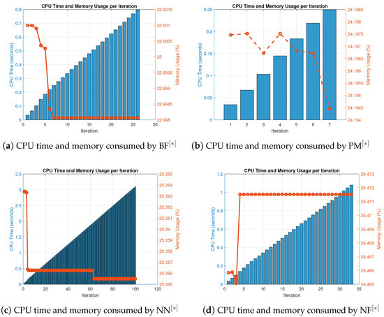
Figure 3.
(a–d) CPU time and memory consumed by parallel schemes utilizing random initial values for solving (36).
In Table 5, the numerical techniques for solving (34) using random initial approximations as provided in Table A1 are displayed together with the number of iterations and percentage convergence. In terms of iterations and percentage convergence, our method outperforms the existing methods PM, in the literature. The computational time and memory used to solve biomedical engineering applications using the MatLab programming software are displayed in Table 6. Our recently developed method finds all solutions parallel to the nonlinear equations using less memory and computational CPU time, resulting in comparatively superior performance. Table 10 shows the overall behavior of the proposed technique. Stability analysis is shown by the number of iterations used and the basic arithmetic operations, and the functions and their derivative evaluations in each iteration step are shown in Table 6 and Table 7. Consistency analysis of the parallel scheme is presented in Table 7 by presenting the overall error of the parallel schemes. By using fewer iterations and fewer fundamental mathematical operations and functions, our recently developed method is more stable in terms of stability than existing methods PM, in the literature. Assessments for parallel approximating all of the roots of (36) are presented; the output of Table 7 is also summarized in Figure 3a–d. In terms of memory and CPU time, our method outperforms other known parallel schemes PM, that choose initial starting values randomly, as shown in Figure 2a–d and Figure 3a–d.
3.2. Biomedical Engineering Application 2: Blood Rheology Model
Blood is a non-Newtonian fluid with changing viscosity under various flow circumstances according to the Blood Rheology Model, which characterizes its flow characteristics. The shear-thinning characteristic of red blood cell alignment, which causes blood viscosity to drop at higher shear rates, is taken into account by this model. Understanding thermodynamics, assisting with medical diagnostics, and enhancing computer simulations of blood flow—especially in vascular illnesses where changing flow can affect health outcomes—all depend on blood rheology models [46] as
Non-linear Equation (39) has the following exact roots, accurate up to fifteen decimal places:
To determine the global convergence behavior, we assume a very rough initial approximations to exact roots as
Table 3 shows the numerical outcomes of these crude initial approximations.
Table 8 and Table 9 show that in terms of residual error at rough initial approximation, our method relatively better approximates all the solutions in biomedical applications with higher decimal places of accuracy using the defined stopping criteria. Figure 4a–d graphically illustrates the residual error verse number of iterations using (41) to approximate all roots of (39) simultaneously. The overall performance in terms of consistency and efficiency are given in Table 8 and Figure 4a–d. Table 4 and Figure 4a–d and Figure 5a–d, clearly indicate that in terms of iterations, basic arithmetic operations memory visualizations, percentage convergence and computer processing time our method perform better than existing methods PM NN.
Table 8.
Error of parallel schemes for solving (39).
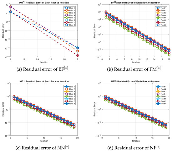
Figure 4.
(a–d) Error graph of parallel scheme for solving (39).
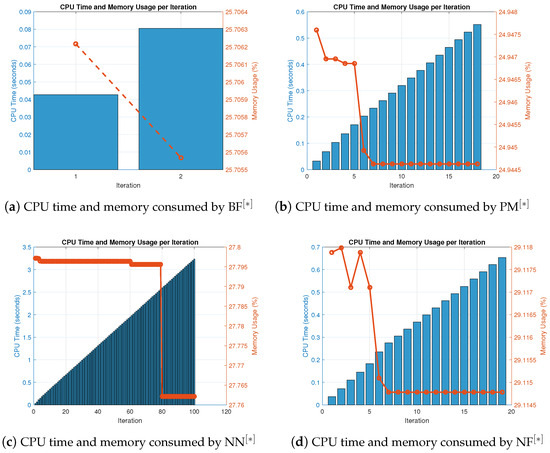
Figure 5.
(a–d) CPU time and memory consumed by parallel schemes for solving (39).
The results for the consistency and stability study of the system for resolving biomedical engineering applications are shown in Table 10, Table 11 and Table 12 and Figure 6a–d, respectively, to verify the global convergence on randomly generated initial vectors.
Table 10.
Iterations and percentage convergence on random initial values.
Table 11.
Memory and computational time in seconds.
Table 12.
Consistency analysis of the parallel schemes for solving (39).
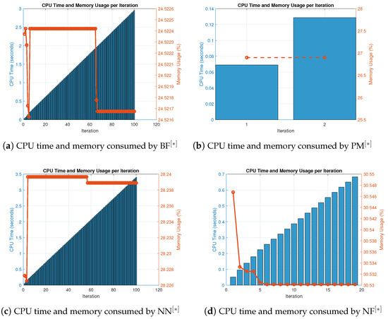
Figure 6.
(a–d). CPU time and memory consumed by parallel schemes for solving nonlinear Equation (39) using random initial values.
Table 10 displays the number of iterations and percentage convergence of the numerical schemes for solving (39) with random initial approximations, as shown in Table A2. In terms of iterations and percentage convergence, our method outperforms the existing methods PM NN in the literature. The computational time and memory used to solve biomedical engineering applications using the MatLab programming software are displayed in Table 11. In terms of memory use and computational CPU time, our novel method performs better than previous methods, taking less CPU time and requiring less memory to locate all solutions parallel to the nonlinear equations. Table 12 depicts the overall behavior of the proposed technique. The consistency analysis of the parallel scheme is shown in Table 12 by displaying the total error of the parallel schemes, and the stability analysis is shown by the number of iterations used and the fundamental mathematical operations. Table 12 also includes the functions and their derivative evaluations in each iteration step in Table 11 and Table 12. In terms of stability, our recently created approach is more stable than existing literary methods PM NN since it uses fewer iterations and fewer fundamental mathematical operations and their functions. Assessments for concurrently approximating all of the roots of (39) in the output of Table 12 are also summarized in Figure 6a–d. In terms of memory and CPU time, our method outperforms other known parallel schemes PM NN that choose initial starting values randomly, as shown in Figure 5a–d and Figure 6a–d.
3.3. Viscosity, Deformability, and Flow: Investigating Blood Rheology
The rheological properties of blood are critical for understanding the circulatory dynamics of a fluid that deforms as it flows. Blood is a non-Newtonian fluid that has shear thinning properties. Viscosity fluctuates with shear rate; elements such as hematocrit content, plasma protein content, and temperature all influence it. It is mostly the result of red blood cells creating rouleaux structures at low shear rates, which increases viscosity. At higher shear rates, these structures rupture and thereby reduce viscosity. Viscoelasticity is another characteristic of blood, which exhibits both fluid and elastic behavior when deformed. The transportation of oxygen and nutrients in physiology depends on these characteristics, but they are also critical in a number of diseases, including diabetes and cardiovascular disorders, where altered rheology affects circulation. The central region’s blood viscosity is significantly higher than that of the peripheral concentric plasma layer.
Plasma viscosity is determined by [46]
where is the core region of hematocrit, is the hematocrit, which is 0.44 at the blood vessel’s inlet. Further,
where is resistivity of blood, and
where cP = centiPoise and 1 Poise (g/(cm S) = 100 cP, is selected in such a way that is always less than 0.6. Putting in (1), we have the following nonlinear equations:
Nonlinear Equation (45) has the following exact roots up to four decimal places:
Table 3 shows the numerical outcomes of these crude initial approximations.
Table 13 and Table 14 show that in terms of residual error at rough initial approximation, our method relatively better approximates all the solutions of biomedical applications with higher decimal place of accuracy using the defined stopping criteria. Figure 7a–d graphically illustrates the residual error verse number of iterations using (47) to approximate all roots of (45) simultaneously. The overall performance in terms of consistency and efficiency is given in Table 13 and Figure 7a–d. Table 15 and Figure 8a–d and Figure 9a–d clearly indicate that in terms of iterations, basic arithmetic operations memory visualizations, percentage convergence, and computer processing time our method performs better than existing methods PM NN.
Table 13.
Error of parallel schemes for solving (45).
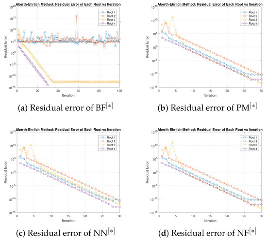
Figure 7.
(a–d) Error graph of parallel scheme for solving (45).
Table 15.
Iterations and percentage convergence on random initial values.
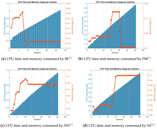
Figure 8.
(a–d) CPU time and memory consumed by parallel schemes for solving (45).
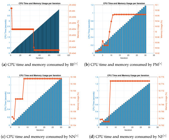
Figure 9.
(a–d) CPU time and memory consumed by parallel schemes for solving nonlinear Equation (45) using random initial values.
To determine the global convergence behavior, we assume a very rough initial approximations to exact roots as
The results of the consistency and stability study of the system for resolving biomedical engineering applications are shown in Table 15, Table 16 and Table 17 and Figure 9a–d, respectively, to verify the global convergence on randomly generated initial vectors.
Table 16.
Memory and computational time in seconds.
Table 17.
Consistency analysis of the parallel schemes for solving (45).
Table 15 displays the number of iterations and percentage convergence of the numerical schemes for solving (45) with random initial approximations, as shown in Table A3. In terms of iterations and percentage convergence, our method outperforms the existing methods PM NN in the literature. The computational time and memory used to solve biomedical engineering applications using the MatLab programming software are displayed in Table 16. In terms of memory use and computational CPU time, our novel method performs better than previous methods, taking less CPU time and requiring less memory to locate all solutions parallel to the nonlinear equations. Table 17 depicts the overall behavior of the proposed technique. The consistency analysis of the parallel scheme is shown in Table 17 by displaying the total error of the parallel schemes, and the stability analysis is shown by the number of iterations used and the fundamental mathematical operations. Table 16 also includes the functions and their derivative evaluations in each iteration step in Table 16 and Table 17. In terms of stability, our recently created approach is more stable than existing literary methods PM NN since it uses fewer iterations and fewer fundamental mathematical operations and their functions. Assessments for concurrently approximating all of the roots of (45) in the output of Table 17 are also summarized in Figure 9a–d. In terms of memory and CPU time, our method outperforms other known parallel schemes PM NN that choose initial starting values randomly, as shown in Figure 8a–d and Figure 9a–d.
3.4. Biomedical Engineering Application
Many biomedical engineering applications use differential equations [47] in their mathematical models, which play an important role in describing dynamic systems that change over time. They are frequently used in pharmacokinetics, where differential equations are used to explain changes in drug concentration in the body, which helps with dosage optimization and the effectiveness of treatment. In addition, IVPs are essential for predicting the course of diseases, modeling their transmission, and assessing the effectiveness of intervention tactics. Initial value problems (IVPs) are utilized in cardiovascular studies to model heart movements and blood flow, which aids in surgical planning and prosthetic device design. The development of medical devices such as pacemakers and neurostimulators is also improved by IVPs, which help simulate electrical activity for muscles and neurons as
Using the approach described in [48], we simulate the solution by using the following polynomial as
where is gamma function, and for we have
Nonlinear Equation (50) has the following exact roots up to three decimal places:
We consider the following rough starting values as
Table 18.
Numerical results of parallel schemes using (50).
In terms of residual error at rough initial approximation, Table 18 and Table 19 demonstrate that our method, when utilizing the defined stopping criteria, approximates all solutions for biomedical applications with greater decimal place of accuracy. Figure 10a–d visually displays the residual error verse number of iterations using (52) to approximate all roots of (50) concurrently. The overall performance in terms of efficiency and consistency is provided in Figure 11a–d and Figure 12a–d and Table 20. Table 19 and Figure 10a–d show that our method outperforms existing methods PM NN in terms of iterations, basic arithmetic operations , memory usage, percentage convergence, and processing time.
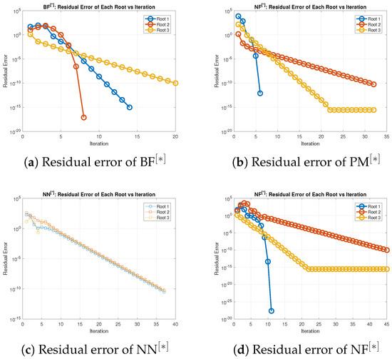
Figure 10.
(a–d) Error graph of the parallel scheme for solving (50).
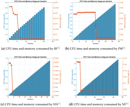
Figure 11.
(a–d) CPU time and memory consumed by parallel scheme for solving (50).
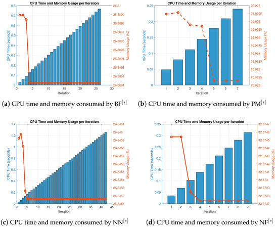
Figure 12.
(a–d) CPU time and memory consumed by parallel schemes for solving (50) utalizing random initial vectors.
Table 20.
Iteations and percentage convergence on random initial values.
The outputs are shown in Table 20, Table 21 and Table 22 and Figure 12a–d to check the global convergence on random initial generated vectors for the consistency and stability study of the scheme for solving biomedical engineering applications.
Table 21.
Memory and computational time in seconds.
Table 22.
Consistancy analysis of the parallel schemes for solving (50).
The number of iterations and percentage convergence of the numerical schemes for solving (50) using random initial approximations, as provided in Table A4, are displayed in Table 20. Compared to the existing methods PM NN in the literature, our approach performs better in terms of iterations and percentage convergence. The computational time and memory used to solve biomedical engineering applications using the MatLab programming software are displayed in Table 20. Our recently developed approach finds all solutions parallel to the nonlinear Equation (50) and has comparatively better performance in terms of memory use and computational CPU time. Table 20 depicts the overall behavior of the proposed technique. The stability analysis is shown by the number of iterations used and the basic arithmetic operations, and the functions and their derivative evaluations in each iteration step are presented in Table 20, Table 21 and Table 22. The consistency analysis of the parallel scheme is presented in Table 22 by displaying the overall error of the parallel schemes. In terms of stability, our recently created approach is more stable than existing literary methods PM NN since it uses fewer iterations and fewer fundamental mathematical operations and their functions. Assessments for concurrently approximating all of the roots of (50) of the output of Table 22 are also summarized in Figure 12a–d. In terms of memory and CPU time, our method outperforms other known parallel schemes PM NN that choose initial starting values randomly, as shown in Figure 11a–d and Figure 12a–d.
3.5. Advantages and Limitations of the Proposed Parallel Scheme
The study provides a novel technique to solve nonlinear equations encountered in biomedical engineering applications by building parallel algorithms. The results indicate significant improvements in computational time, convergence rate, and memory utilization when compared to existing schemes. However, these findings must be placed within the larger framework of numerical methods for nonlinear biomedical engineering problems. The newly developed parallel method’s strengths include:
- -
- Computational Efficiency: Parallel techniques save significant calculation time, as demonstrated by their use in four separate biological applications.
- -
- Better Convergence Rate: Compared to conventional schemes, the suggested scheme assures fast convergence by determining solutions more effectively in fewer iterations.
- -
- Memory Efficiency: A comparison of memory utilization demonstrates the scheme’s applicability in resource-constrained environments.
- -
- Error Analysis: Including error graphs shows how accurate the solutions are and confirms that the approach is reliable.
- -
- The Percentage Computational Efficiency: The quantitative comparison highlights a method’s competitive advantage, especially in large-scale problems.
Although the suggested parallel approaches improve computational efficiency [49,50], convergence rate, and memory optimization in three biomedical applications, there are significant drawbacks to the method. Its applicability to extremely high-dimensional issues and reliance on parallel hardware may limit its utility in resource-constrained settings. It is necessary to investigate the error behavior at the edge cases, like ill-conditioned systems. The method will be optimized for various computer architectures, its scalability will be improved, and experiments with applications to stochastic and multi-scale models will be conducted in the future.
4. Conclusions
Here, we developed new parallel techniques to simultaneously locate all the roots of nonlinear equations. The newly created parallel scheme has a ninth-order convergence according to the convergence analysis. In order to solve biomedical engineering problems, the effectiveness and stability of recently established parallel schemes are evaluated by analyzing rough initial starting values. The global convergence behavior is further investigated with random starting test vectors. In terms of memory, number of iterations, percentage convergence, number of basic arithmetic operations, function and derivative evaluations in each iteration, residual error graph, and computational time in seconds, our newly developed methods outperform existing methods PM NN NF
In the future, we will develop higher-order inverse parallel algorithms to address more complex problems in epidemic modeling and biomedical engineering. In order to increase the accuracy and efficiency of computational models, additional fractional derivative notations will be used. Advanced methods will be employed to forecast and model dynamic, complex systems. They will also contribute to the development of novel methods for minimizing epidemics and improving health outcomes. Finally, in the future, we aim to bridge the gap between theoretical advances and practical applications in biomedical sciences.
Author Contributions
Conceptualization, M.S. and B.C.; methodology, M.S.; software, M.S.; validation, M.S.; formal analysis, B.C.; investigation, M.S.; resources, B.C.; writing—original draft preparation, M.S. and B.C.; writing—review and editing, B.C.; visualization, M.S. and B.C.; supervision, B.C.; project administration, B.C.; funding acquisition, B.C. All authors have read and agreed to the published version of the manuscript.
Funding
The work is supported by the Free University of Bozen-Bolzano (IN200Z SmartPrint) and by Provincia Autonoma di Bolzano/Alto Adige—Ripartizione Innovazione, Ricerca, Università e Musei (CUP codex I53C22002100003 PREDICT). Bruno Carpentieri is a member of the Gruppo Nazionale per il Calcolo Scientifico (GNCS) of the Istituto Nazionale di Alta Matematica (INdAM) and this work was partially supported by INdAM-GNCS under Progetti di Ricerca 2024.
Data Availability Statement
Data are contained within the article.
Conflicts of Interest
The authors declare that there are no conflicts of interest regarding the publication of this article.
Abbreviations
| The following abbreviations are used in this manuscript: | |
| CPU time | Computational Time Seconds |
| Max-It | Maximum Iterations |
| Max-Error | Maximum Error |
| Per-Con | Percentage Convergence |
| Existing Parallel Methods | |
| Residual Error | |
| Newly Developed Methods | |
Appendix A
The random initial starting vector is employed in biomedical engineering Appliaction 1 to show the global convergence of the numerical schemes, as presented in Table A1.
Table A1.
Random initial vectors.
Table A1.
Random initial vectors.
| Ran-Test | |||
|---|---|---|---|
| 1 | |||
| 2 | |||
| 3 | |||
| 4 | |||
| 5 |
The random initial starting vector is employed in biomedical engineering Appliaction 3 to show the global convergence of the numerical schemes, as presented in Table A2.
Table A2.
Random initial vectors.
Table A2.
Random initial vectors.
| Ran-Test | |||||
|---|---|---|---|---|---|
| 1 | |||||
| 2 | |||||
| 3 | |||||
| 4 | |||||
| 5 |
The random initial starting vector is employed in biomedical engineering Appliaction 2 to show the global convergence of the numerical schemes, as presented in Table A3.
Table A3.
Random initial vectors.
Table A3.
Random initial vectors.
| Ran-Test | ||||
|---|---|---|---|---|
| 1 | ||||
| 2 | ||||
| 3 | ||||
| 4 | ||||
| 5 |
The random initial starting vector is employed in engineering Application 4 to show the global convergence of the numerical schemes, as presented in Table A4.
Table A4.
Random initial vectors.
Table A4.
Random initial vectors.
| Ran-Test | |||
|---|---|---|---|
| 1 | |||
| 2 | |||
| 3 | |||
| 4 | |||
| 5 |
References
- Cropley, D.H. Homo Problematis Solvendis–Problem-Solving Man: A History of Human Creativity; Springer: Berlin/Heidelberg, Germany, 2019. [Google Scholar]
- Zitouni, F.; Harous, S. Integrating the Opposition Nelder–Mead Algorithm into the Selection Phase of the Genetic Algorithm for Enhanced Optimization. Appl. Syst. Innov. 2023, 6, 80. [Google Scholar] [CrossRef]
- Rashed, R. The Development of Arabic Mathematics: Between Arithmetic and Algebra; Springer Science and Business Media: Dordrecht, The Netherlands, 2013; Volume 156, Chapter 3; pp. 85–146. [Google Scholar]
- Schneider, C.; Zima, E.V. (Eds.) Advances in Computer Algebra; Springer: Berlin/Heidelberg, Germany, 2018. [Google Scholar]
- Richardson, S. Mathematics teachers’ development, exploration, and advancement of technological pedagogical content knowledge in the teaching and learning of algebra. Contemp. Issues Technol. Teach. Educ. 2009, 9, 117–130. [Google Scholar]
- Zhang, T. Research on Integrated application of Advance Mathematics and linear Algebra. Highlights Sci. Eng. Tech. 2023, 56, 630–634. [Google Scholar] [CrossRef]
- Sbalzarini, I.F. Modeling and simulation of biological systems from image data. Bioessays 2013, 35, 482–490. [Google Scholar] [CrossRef]
- Resat, H.; Petzold, L.; Pettigrew, M.F. Kinetic modeling of biological systems. Comput. Syst. Biol. 2009, 541, 311–335. [Google Scholar]
- Tobler, A.; Mühlebach, S. Intravenous phenytoin: A retrospective analysis of Bayesian forecasting versus conventional dosing in patients. Int. J. Clin. Pharm. 2013, 35, 790–797. [Google Scholar] [CrossRef] [PubMed]
- Xi, Y.; Zhao, J.; Bennett, J.R.; Stacy, M.R.; Sinusas, A.J.; Wang, G. Simultaneous CT-MRI reconstruction for constrained imaging geometries using structural coupling and compressive sensing. IEEE Trans. Biomed. Eng. 2015, 63, 1301–1309. [Google Scholar] [CrossRef] [PubMed]
- Kipouros, T.; Jaeggi, D.; Dawes, B.; Parks, G.; Savill, M.A.; Clarkson, P.J. Insight into high-quality aerodynamic design spaces through multi-objective optimization. CMES Comput. Model. Eng. Sci. 2008, 37, 1–23. [Google Scholar]
- Landman, D.J.; Simpson, D.V.; Peter, P. Response surface methods for efficient complex aircraft configuration aerodynamic characterization. J. Aircraf. 2007, 44, 1189–1195. [Google Scholar] [CrossRef]
- Liu, Y. Bibliometric Analysis of Weather Radar Research from 1945 to 2024: Formations. Develop. Trends Sens. 2024, 24, 3531. [Google Scholar]
- Akhtar, Z.B. Exploring Biomedical Engineering (BME): Advances within Accelerated Computing and Regenerative Medicine for a Computational and Medical Science Perspective Exploration Analysis. J. Emerg. Med. OA 2024, 2, 1–23. [Google Scholar] [CrossRef]
- Akbar, S.; Shah, S.R. Mathematical Modeling of blood flow dynamics in the cardiovascular system: Assumptions, considerations, and simulation results. J. Curr. Med. Res. Opin. 2024, 7, 2216–2225. [Google Scholar]
- Srivastava, V.; Tripathi, D.; Srivastava, P.K.; Kuharat, S.; Bég, O.A. Mathematical Modeling of Oxygen Diffusion from Capillary to Tissues during Hypoxia through Multiple Points Using Fractional Balance Equations with Memory. Crit. Rev.™ Biomed. Eng. 2024, 52, 1–10. [Google Scholar] [CrossRef] [PubMed]
- Tarasova, I.; Kukhareva, I.; Kupriyanova, D.; Temnikova, T.; Gorbatovskaya, E.; Trubnikova, O. Electrical Activity Changes and Neurovascular Unit Markers in the Brains of Patients after Cardiac Surgery. Eff. -Multi-Task Cogn. Training. Biomed. 2024, 12, 756. [Google Scholar]
- Han, Y.; Chen, Y.; Ong, C.; Chen, J.; Hicks, J.; Teran, J. A Neural Network Model for Efficient Musculoskeletal-Driven Skin Deformation. ACM Trans. Graph. (TOG) 2024, 43, 1–12. [Google Scholar] [CrossRef]
- Yang, X.; Wang, W.; Ma, J.L.; Qiu, Y.L.; Lu, K.; Cao, D.S.; Wu, C.K. BioNet: A large-scale and heterogeneous biological network model for interaction prediction with graph convolution. Briefings Bioinform. 2022, 23, bbab491. [Google Scholar] [CrossRef]
- Jin, S.; Zeng, X.; Xia, F.; Huang, W.; Liu, X. Application of deep learning methods in biological networks. Briefings Bioinform. 2021, 22, 1902–1917. [Google Scholar] [CrossRef] [PubMed]
- Jajarmi, A.; Baleanu, D. A new iterative method for the numerical solution of high-order non-linear fractional boundary value problems. Front. Phys. 2020, 8, 220. [Google Scholar] [CrossRef]
- Sazaklioglu, A.U. An iterative numerical method for an inverse source problem for a multidimensional nonlinear parabolic equation. Appl. Numer. Math. 2024, 198, 428–447. [Google Scholar] [CrossRef]
- Batiha, B. Innovative Solutions for the Kadomtsev–Petviashvili Equation via the New Iterative Method. Math. Prob. Eng. 2024, 2024, 5541845. [Google Scholar] [CrossRef]
- Halilu, A.S.; Waziri, M.Y. A transformed double step length method for solving large-scale systems of nonlinear equations. J. Numer. Math. Stoch. 2021, 9, 20–23. [Google Scholar]
- Abbott, J.P.; Brent, R.P. Fast local convergence with single and multistep methods for nonlinear equations. Anziam J. 1975, 19, 173–199. [Google Scholar] [CrossRef]
- Ahmad, F.; Tohidi, E.; Carrasco, J.A. A parameterized multi-step Newton method for solving systems of nonlinear equations. Numer. Alg. 2016, 71, 631–653. [Google Scholar] [CrossRef]
- Rafiq, A.; Rafiullah, M. Some multi-step iterative methods for solving nonlinear equations. Comp. Math. Appl. 2009, 58, 1589–1597. [Google Scholar] [CrossRef]
- Erfanifar, R.; Hajarian, M. A new multi-step method for solving nonlinear systems with high efficiency indices. Numer. Alg. 2024, 97, 959–984. [Google Scholar] [CrossRef]
- Kabir, M.M.; Khajeh, A.; Abdi Aghdam, E.; Yousefi Koma, A. Modified Kudryashov method for finding exact solitary wave solutions of higher-order nonlinear equations. Math. Methods Appl. Sci. 2011, 34, 213–219. [Google Scholar] [CrossRef]
- He, J.H. Review on some new recently developed nonlinear analytical techniques. Int. J. Nonlinear Sci. Numer. Simul. 2000, 1, 51–70. [Google Scholar] [CrossRef]
- He, J.H. Homotopy perturbation method: A new nonlinear analytical technique. Appl. Math. Comput. 2003, 135, 73–79. [Google Scholar] [CrossRef]
- Falcão, M.I.; Miranda, F.; Severino, R.; Soares, M.J. Weierstrass method for quaternionic polynomial root-finding. Math. Methods Appl. Sci. 2018, 41, 423–437. [Google Scholar] [CrossRef]
- Nedzhibov, G.H. Local convergence of the Inverse Weierstrass method for simultaneous approximation of polynomial zeros. Int. J. Math. Anal. 2016, 10, 1295–1304. [Google Scholar] [CrossRef][Green Version]
- Shams, M.; Bruno, C. Efficient inverse fractional neural network-based simultaneous schemes for nonlinear engineering applications. Fractal Fract. 2023, 7, 849. [Google Scholar] [CrossRef]
- Lopes, L.G.; Machado, R.N. A New Ehrlich-Type Sixth-Order Simultaneous Method for Polynomial Complex Zeros. VETOR-Revista de Ciências Exatas e Engenharias 2023, 33, 52–59. [Google Scholar] [CrossRef]
- Nourein, A.W. An improvement on Nourein’s method for the simultaneous determination of the zeroes of a polynomial (an algorithm). J. Comput. Appl. Math. 1977, 3, 109–112. [Google Scholar] [CrossRef]
- Zhang, X.; Peng, H.; Hu, G. A high order iteration formula for the simultaneous inclusion of polynomial zeros. Appl. Math. Comput. 2006, 179, 545–552. [Google Scholar] [CrossRef]
- Petkovic, M. Iterative Methods for Simultaneous Inclusion of Polynomial Zeros; Springer: Berlin/Heidelberg, Germany, 2006; Volume 1387. [Google Scholar]
- Zein, A. A general family of fifth-order iterative methods for solving nonlinear equations. Eur. J. Pure Appl. Math. 2023, 16, 2323–2347. [Google Scholar] [CrossRef]
- Rafiq, N.; Akram, S.; Shams, M.; Mir, N.A. Computer geometries for finding all real zeros of polynomial equations simultaneously. Comput. Mater. Contin. 2021, 69, 2636–2651. [Google Scholar] [CrossRef]
- Petković, M.S.; Petković, L.D.; Džunić, J. On an efficient simultaneous method for finding polynomial zeros. Appl. Math. Lett. 2014, 28, 60–65. [Google Scholar] [CrossRef]
- Wang, D.R.; Wu, Y.J. Some modifications of the parallel Halley iteration method and their convergence. Computing 1987, 38, 75–87. [Google Scholar] [CrossRef]
- Petković, M.S.; Rančić, L.; Milošević, M. The improved Farmer–Loizou method for finding polynomial zeros. Int. J. Comput. Math. 2012, 89, 499–509. [Google Scholar] [CrossRef]
- Jia, Y.; Sun, J.; Zhao, Y.; Tang, K.; Zhu, R.; Zhao, W.; Chen, W. Chinese patent medicine for osteoporosis: A systematic review and meta-analysis. Bioengineered 2022, 13, 5581–5597. [Google Scholar] [CrossRef] [PubMed]
- Yu, X.; Ye, C.; Xiang, L. Application of artificial neural network in the diagnostic system of osteoporosis. Neurocomputing 2016, 214, 376–381. [Google Scholar] [CrossRef]
- Shams, M. On a Stable Multiplicative Calculus-Based Hybrid Parallel Scheme for Nonlinear Equations. Mathematics 2024, 12, 3501. [Google Scholar] [CrossRef]
- Shams, M.; Carpentieri, B. On highly efficient fractional numerical method for solving nonlinear engineering models. Mathematics 2023, 11, 4914. [Google Scholar] [CrossRef]
- Subburayan, V. An hybrid initial value method for singularly perturbed delay differential equations with interior layers and weak boundary layer. Ain. Shams Eng. J. 2018, 9, 727–733. [Google Scholar] [CrossRef]
- Shams, M.; Kausar, N.; Agarwal, P.; Oros, G.I. Efficient iterative scheme for solving non-linear equations with engineering applications. Appl. Math. Sci. Eng. 2022, 30, 708–735. [Google Scholar] [CrossRef]
- Torkashvand, V. Efficient two-step with memory methods and their dynamics. Math. Comput. Sci. 2024, 5, 80–92. [Google Scholar]
Disclaimer/Publisher’s Note: The statements, opinions and data contained in all publications are solely those of the individual author(s) and contributor(s) and not of MDPI and/or the editor(s). MDPI and/or the editor(s) disclaim responsibility for any injury to people or property resulting from any ideas, methods, instructions or products referred to in the content. |
© 2024 by the authors. Licensee MDPI, Basel, Switzerland. This article is an open access article distributed under the terms and conditions of the Creative Commons Attribution (CC BY) license (https://creativecommons.org/licenses/by/4.0/).