Stroke Dataset Modeling: Comparative Study of Machine Learning Classification Methods

Abstract

Stroke prediction is a vital research area due to its significant implications for public health. This comparative study offers a detailed evaluation of algorithmic methodologies and outcomes from three recent prominent studies on stroke prediction. Ivanov et al. tackled issues of imbalanced datasets and algorithmic bias using deep learning techniques, achieving notable results with a 98% accuracy and a 97% recall rate. They utilized resampling methods to balance the classes and advanced imputation techniques to handle missing data, underscoring the critical role of data preprocessing in enhancing the performance of Support Vector Machines (SVMs). Hassan et al. addressed missing data and class imbalance using multiple imputations and the Synthetic Minority Oversampling Technique (SMOTE). They developed a Dense Stacking Ensemble (DSE) model with over 96% accuracy. Their results underscore the efficiency of ensemble learning techniques and imputation for handling imbalanced datasets in stroke prediction. Bathla et al. employed various classifiers and feature selection techniques, including SMOTE, for class balancing. Their Random Forest (RF) classifier, combined with Feature Importance (FI) selection, achieved an accuracy of 97.17%, illustrating the positive impact of RF and relevant feature selection on model performance. A comparative analysis indicated that Ivanov et al.’s method achieved the highest accuracy rate. However, the studies collectively highlight that the choice of models and techniques for stroke prediction should be tailored to the specific characteristics of the dataset used. This study emphasizes the importance of effective data management and model selection in enhancing predictive performance.

1. Introduction

Stroke remains one of the most prevalent global health disorders, ranking as the third leading cause of death and disability worldwide. Strokes occur when the blood supply to the brain is interrupted or when there is bleeding within the brain, resulting in significant morbidity and mortality. According to the World Stroke Organization, approximately 15 million people suffer strokes annually, with a one-in-four chance that individuals over the age of 25 will experience a stroke during their lifetime. This widespread and devastating impact on patients, families, and healthcare resources underscores the critical need for accurate prediction and preventive measures [1].

Since 2015, stroke has become the foremost cause of death and disability in China, exacerbated by factors such as an aging population, urbanization, and unhealthy lifestyles [2]. The advent of artificial intelligence (AI), particularly machine learning (ML), offers promising tools for stroke prediction. These technologies leverage large datasets and sophisticated algorithms to identify risk factors, predict outcomes, and optimize preventive strategies.

This study aimed to compare methodologies and findings from fundamental research papers that employ practical classification analyses and comprehensive approaches for stroke prognostication, utilizing datasets available on the Kaggle platform. These studies consider various demographic, medical history, lifestyle, and physiological features crucial for predicting stroke. However, shared challenges such as missing data and class imbalance in the observations can impede predictive accuracy and need addressing.

This article reviews three significant studies by Ivanov et al., Hassan et al., and Bathla et al., all published in the Scopus database post-August 2023. The comparison focuses on standard classification metrics such as accuracy, precision, sensitivity, and specificity, with each selected methodology demonstrating evaluation parameters above 95%. The benchmarking process identifies essential steps in developing effective algorithmic methodologies, including handling missing data, managing unbalanced datasets, selecting appropriate classification models and parameters, and assessing classification results. As a result, the methodology creates an innovative solution implemented through a machine learning model.

One of the main issues with stroke prediction datasets is class imbalance, where 95% of records belong to one class, and only 5% belong to the stroke class. Addressing this imbalance is crucial to avoiding model biases that favor the majority class, which can lead to suboptimal performance in predicting the minority class. Practical solutions to these challenges are vital for developing accurate and reliable stroke risk prediction models.

A study [3] by Ivanov et al. emphasized addressing imbalanced data and missing values through advanced machine learning techniques and optimization models. They applied Support Vector Machines (SVMs), Decision Trees (DTs), and Random Forests (RFs) using class balancing techniques and robust imputation methods. The SVM model achieved the highest accuracy (98%) and recall with specific parameter configurations, demonstrating superior predictive capability. Their Random Forest and decision tree models also performed well, highlighting the importance of model selection and configuration.

In contrast, a study [4] by Hassan et al. utilized multiple imputation techniques for handling missing data, with MICE (Multiple Imputation by Chained Equations) offering the best results. To address data imbalance, the Synthetic Minority Over-sampling Technique (SMOTE) was applied. The Dense Stacking Ensemble (DSE) model employed by Hassan et al. showed exceptional performance, particularly on balanced datasets, affirming the efficacy of their chosen imputation and ensemble learning techniques.

A study [5] by Bathla et al. combined multiple feature selection processes and classifiers. They used SMOTE for class balancing and examined various classifiers, ultimately identifying Random Forest with Feature Importance as the most effective, achieving an accuracy of 97.17%. This study demonstrated the significant impact of feature selection and class balancing on model performance.

The published studies also complement the issues of data imbalance and missing data by drawing attention to the selection of features and the tuning of algorithms. They reveal that with the right choice of features and efficient algorithms, researchers can construct models that predict strokes more efficiently and give an idea about how to prevent strokes or treat the affected individual.

Based on the comparison of the findings from the reviewed studies, it was found that there is a diversification of methodologies and research studies that all contribute to a better understanding of stroke prediction. Ivanov et al. emphasize SVM and the implementation of resampling techniques; Hassan et al.’s application of SMOTE and ensemble, and Bathla et al.’s hybrid system development, present the field’s current and most potentially developing scenario. Each approach is advantageous and disadvantageous, highlighting the complications in predicting a stroke and emphasizing the requirement for further advancements in the topic.

Incorporating machine learning in stroke prediction is one step in improving modern healthcare analytics. Since dealing with imbalanced data, missing data, and feature selection are critical, they call for effective solutions and proper assessment to improve accurate models. This article sets the stage for a detailed exploration of the methodologies and results presented in the reviewed studies, offering a critical evaluation of their contributions and identifying best practices for future research.

The comparative analysis reveals that while each study presents unique methodologies and strengths, a critical takeaway is the importance of tailoring model selection and techniques to the specific characteristics of the dataset. This research demonstrates the valuable contributions of AI and machine learning to stroke prediction, highlighting the necessity for ongoing advancements to enhance predictive accuracy and, ultimately, improve patient outcomes.

In conclusion, predicting strokes using machine learning offers substantial early diagnosis and prevention opportunities. This research synthesized methodologies and findings from various studies, providing insights into best practices and areas for further improvement. Integrating effective data handling techniques and model optimization remains crucial to advancing stroke prediction models and positively impacting global health outcomes. We highlight a paper [6], Asadi et al., 2024, in which the authors systematically review articles published up to August 2023 with the subject of stroke prediction.

2. Materials and Methods

2.1. Comprehensive Models for Stroke Prevention

Advancements in stroke prevention modeling have enriched our understanding and refined preventive strategies. Several essential modeling techniques are utilized in this area:

• Risk Assessment Models: Risk assessment models are invaluable for identifying individuals at high risk for stroke early. These models consider various demographic factors (e.g., age, gender) and lifestyle habits (e.g., smoking, alcohol consumption). By evaluating the probability of stroke occurrence, these models enable the development of personalized prevention plans [7].
• Pharmacological Intervention Models: Pharmacological intervention models evaluate the effectiveness of anticoagulants, antiplatelets, and antihypertensives in stroke prevention [8]. These models help determine the optimal dosing regimens and identify patient profiles that would benefit most from these treatments, ensuring that therapies are effective and appropriately dosed [9].
• Lifestyle Intervention Models: These models assess the impact of lifestyle modifications, such as dietary changes and physical activity, on stroke risk [10]. Based on individual health profiles, they provide tailored recommendations aimed at reducing stroke incidence and contribute to the formulation of personalized prevention strategies.
• Screening Program Models: Screening models compare the cost-effectiveness of various screening approaches, including those targeting atrial fibrillation, a known stroke risk factor [11,12]. These models guide public health officials in developing effective community-based screening protocols to reduce stroke incidence.
• Patient Education Models: Patient education models evaluate the impact of different educational initiatives on stroke prevention [13]. These models identify the most effective educational strategies and assist healthcare providers in implementing programs that enhance public knowledge about stroke risk factors and prevention.
• Models for Atrial Fibrillation (AF) Management: The Atrial Fibrillation Better Care (ABC) pathway provides a systematic framework for managing AF, aiming to reduce stroke and adverse events through continuous risk assessment. Tools like the CHA₂DS₂-VASc score [14] are used for selecting patients for anticoagulation therapy. However, recent approaches emphasize dynamic risk assessment to manage bleeding risks and target at-risk patients for early intervention [15].

By integrating these diverse modeling frameworks, clinicians and researchers can develop more effective stroke prevention strategies tailored to individual patient needs and dynamic clinical conditions.

2.2. Classification Methodologies for Addressing Class Imbalance and Missing Data

Addressing class imbalance and missing data in machine learning is crucial, particularly in medical applications such as stroke prediction. Imbalanced datasets can lead to models that disproportionately favor the majority class, resulting in poor predictive performance for the minority class, which is often the critical condition (e.g., stroke). In three comment articles, this issue was described as one that significantly influences the performance of the forecasts and models.

The situation where the classes are imbalanced and missing values are in the data can be considered an issue as far as machine learning is concerned, particularly when it comes to medical applications. In recent years, the classification of imbalanced datasets has been one of the main problems for machine learning modeling. Imbalanced datasets with two classes mean one class dominates over another one. Thus, when a machine learning model is created that focuses on frequently privileged samples, it typically ignores less common but more critical samples. For example, in the case of stroke prediction, if the number of samples with stroke is significantly less compared to the number of samples without stroke, then the outcomes of a model cannot identify people at high risk.

With the continuous extension of data availability in complex, large-scale, and networked systems, such as security, finance, and the Internet, it is essential to elevate the basic understanding of knowledge in this area. Even though existing techniques have revealed great success in many real-world applications, the issue of learning from imbalanced data is new. Therefore, this problem needs more engagement from researchers.

Several survey articles related to the imbalanced learning area have been published in the past few years. In [16], the authors review SVM’s weakness in handling imbalanced datasets and describe why there are better choices than the traditional under-sampling approaches. Another survey about class imbalance learning methods for SVM was collected in [17]. The purpose of the survey was to review different data preprocessing and algorithmic approaches to improve the performance of SVM in learning from imbalanced datasets. The critical issue in knowledge discovery and data engineering is imbalanced learning [18]. Their concentration was to present a challenging review of the nature of the issue, existing evaluation metrics, and state-of-the-art technologies utilized to assess learning performance under the imbalanced learning scenario. They used some significant assessments as a perfect reference for present and subsequent knowledge discoveries.

Likewise, missing values in data are a disadvantage in model training and assessment. This situation occurs when missing or erroneous information that contributes to the formation of subsets of features is present in the learning samples. This is even more dangerous in contexts like medicine since risk scoring relies more on accurate information.

Solving these problems is achieved through resampling to balance the classes and other complex imputation methods to handle missing values. By addressing these problems, the efficacy and efficiency of theoretical estimations can be significantly enhanced by applying them to medicine in diagnosis and patient care.

2.2.1. Challenges: Imbalanced Datasets and Missing Data

-

Imbalanced Datasets: With an uneven distribution of classes, models may become biased towards the majority class, neglecting the minority class.

-

Missing Data: Missing or erroneous entries can significantly impact model accuracy, particularly in high-stakes medical fields.

2.2.2. Solutions: Resampling Techniques and Imputation Methods

-

Resampling Techniques: Balancing the classes via resampling (e.g., SMOTE) can mitigate biases.

-

Imputation Methods: Addressing missing data through mean or median imputation or advanced techniques like MICE preserves dataset integrity.

2.3. Methodology Overview

Methodology A: Ivanov et al. [3] addressed missing data by employing mean or median imputation or removing incomplete entries. They tackled class imbalance using synthetic data augmentation for the minority class. The methodology applies Random Forest, Decision Tree, and SVM models, evaluated using accuracy, precision, sensitivity, specificity, and AUC-ROC metrics.

Methodology B: Hassan et al. [4] utilized three imputation techniques: mean value replacement, MICE, and age group-based imputation. They balanced the dataset with SMOTE, which was applied cautiously to avoid overfitting. The methodology uses various models, including logistic regression, neural networks, and ensemble methods, assessed through k-fold cross-validation.

Methodology C: Bathla et al. [5] used SMOTE for data balancing and mean imputation for missing data. They applied feature selection techniques (MI, PC, FI) and evaluated five classifiers: Naive Bayes, SVM, Random Forest, AdaBoost, and XGBoost. Ten-fold cross-validation was used to evaluate performance, with metrics such as accuracy, sensitivity, specificity, precision, and F-measure.

2.3.1. Methodology A

We considered the methodology proposed by Ivanov and co-authors [3], 2023, which we call Methodology A for brevity. In the article, the authors suggest that the missing data be replaced with the relevant characteristic’s mean value or median, or they can be removed from the dataset. The proposed methodology solves the imbalanced data problem by augmenting the observations of the minority class by creating new synthetic examples. This approach helps balance the dataset while improving the performance of the classification model. In addition, the methodology reduces observations of the majority class. The methodology is applied through the three models: Random Forest, Decision Tree, and SVM. The observations are split into training and test subsets using the command train test split with parameter test size = 0.4. The methodology is evaluated by calculating accuracy, precision, sensitivity, specificity, and AUC-ROC parameters.

2.3.2. Methodology B

We considered the methodology proposed by Hassan and co-authors [4], 2024, which, for brevity, we call Methodology B. Experiments were conducted using three different missing data handling techniques. First, the missing values were replaced with the mean value of the corresponding characteristic. Second, Multivariate Imputation by Chained Equations (MICE) was performed, which uses regression models to predict missing values based on information from other variables. Third, age group-based imputation was used to replace missing BMI values with the mean value for the respective age group (4 groups: 0–20, 21–40, 41–60, and 61–80). Methodology B uses the SMOTE technique as a data balancing tool, which increases the representation of the minority class. The paper emphasizes that an incorrect application of SMOTE can lead to overfitting, which requires careful management of method parameters. The paper evaluates SMOTE’s performance by comparing the model’s performance on balanced and unbalanced datasets. This also includes a consideration of potential drawbacks of the method, such as the risks of overfitting and data reduction by reducing examples from the majority class. The methodology relies on basic and advanced models such as logistic regression, neural networks, TabNet, and gradient-boosting methods (XGBoost, CatBoost, etc.) for classification analysis. The dataset is divided into training and testing data using a 70:30 ratio to evaluate the results. Then, k-fold cross-validation is used to evaluate models. The results are based on various performance metrics. An advantage of the classification analysis is that the authors presented the elements of confusion matrices for the models used, through which the necessary metrics can be calculated.

2.3.3. Methodology C

We considered the methodology proposed by Bathla and co-authors [5], 2024, which we call Methodology C for brevity. The original dataset included 249 patients diagnosed with stroke and 4861 non-stroke individuals, and the researchers used the SMOTE technique to balance the data. Then, the mean imputation technique was used in all subsequent analyses to deal with the missing data in the dataset. This technique replaces all the missing values with the mean of other values within the same feature to ensure the dataset is complete. Afterwards, the imputed study used three feature selection techniques, including Mutual Information (MI), Pearson’s Correlation (PC), and Feature Importance (FI). MI aims to quantify the extent of the relationship between features and the target variable as well as the strength of the association. In contrast, PC seeks to quantify the nature of the relationship between the measures and the strength of the relationship. FI evaluates the significance of each feature in the prediction model.

Five classifiers were used to test stroke prediction performance. The algorithms were Naive Bayes (NB), Support Vector Machine, Random Forest, Adaboost, and XGBoost. The performance of each classifier was tested using the cross-validation techniques, particularly the cross-validation by ten folds, which splits the data into ten sets. The model was trained on nine subsets and tested on the remaining subset, and the process was carried out ten times. The effectiveness of the implementation was measured by three criteria: accuracy, sensitivity, and specificity, as well as precision and F-Measure. The practical feature selection methods and classifier combinations were determined, revealing a detailed picture of the best practice models of stroke prevention.

2.4. Application of the Methodology

2.4.1. Description of the Dataset

The dataset used in this analysis is publicly available in Kaggle’s Stroke Prediction Dataset [19]. The dataset is in CSV format and contains 5110 observations with 11 variables, of which 10 are independent, and 1 is the target (

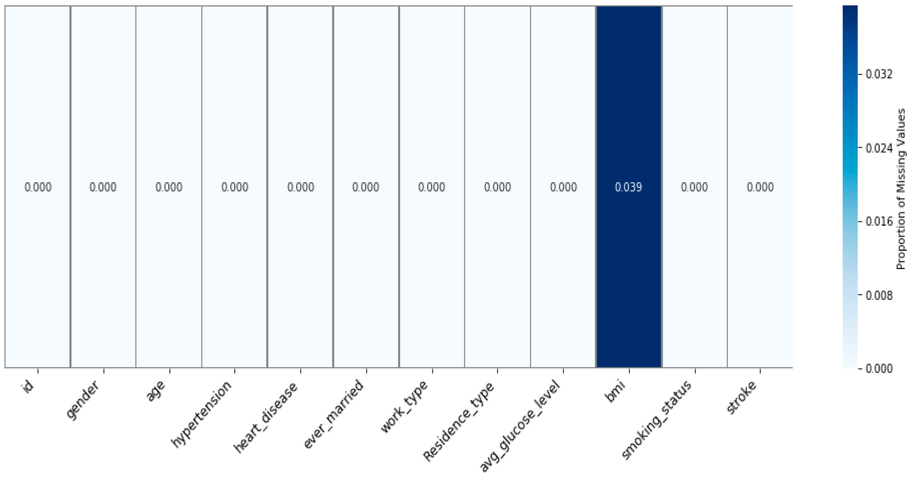
Table 1. The characteristics of the dataset.

Number	Variables Name
1	id (abbr. for identifier)
2	gender
3	age
4	hypertension
5	heart_disease
6	ever_married
7	work_type
8	Residence_type
9	avg_glucose_level
10	bmi (abbr. for body mass index)
11	smoking_status
12	stroke

). The target variable, called “stroke”, indicates whether there is a risk of stroke or not. The value of “0” indicates no risk of stroke, while a value of “1” signifies a risk of stroke. The dataset shows a significant class imbalance, with about 95.13% of observations indicating no risk of stroke and only 4.87% showing a risk of stroke. There are missing values (Figure 1) that can result from incomplete data collection, or some errors related to data entry. Identifying these missing values is a prerequisite to accurately solving the problem and finding the best approach to address the underlying issues in the data gathering and preparation. Structuring the dataset and the issue of missing data points within the dataset are critical features that must be taken into account during the preprocessing process and the actual modeling.

2.4.2. Missing Values

Handling missing values is critical to the effectiveness of machine learning, and the choice between imputation and imputation depends on the particular characteristics of the dataset and the number of missing values. The variable “BMI” (Table 1) contained 201 missing values out of 5110 observations, representing about 3.93% of the data (Figure 1). The authors’ approaches to handling missing values in the three studies demonstrate a diversity in methodology and strategies for dealing with incomplete data.

The authors considered several main strategies and conducted experiments to deal with missing values: exclusion of cases with missing information or using mean, median, and mode for average values. Subsequently, they also excluded the observations where they observed missing values since the number of instances was relatively lesser; using imputation would skew the results. Further, the authors dropped the “id” column (Table 1) as this column only has numerical values for the unique identification of patients, and such columns do not include information relevant to the risk of stroke. Due to all these steps, the data frame was reduced to 4909 rows and 11 columns, and then used for analysis and modeling.

Imputation Methods to Address Missing Values—Methodology A

Ivanov et al. detailed experiments using mean imputation and data removal methods in their article. However, data removal delivered superior results to imputation, so they incorporated it into their Methodology A.

Imputation Methods to Address Missing Values—Methodology B

The authors (Hassan et al.) of Methodology B chose to use imputation techniques instead of removing rows with missing values to avoid losing data and insights. They carefully chose imputation techniques to mitigate the risk of introducing assumptions or biases. The effectiveness of these imputation methods was evaluated in comparison to the traditional approach of listwise deletion, aiming to balance data utility with accuracy and minimize any potential bias introduced by the imputation process. Their study employed three distinct imputation methods to address missing values effectively. Mean imputation: this imputation technique fills in missing values about the mean of the variable value; this methodology does not negatively affect data integrity and analysis arising from incomplete data. It permits the maximum information available, resulting in better and more stable results. Multivariate Imputation by Chained Equations (MICE): multiple imputations and sequential regression together in MICE are superior to filling in missing variables more accurately. This approach improves imputation accuracy and reliability by incorporating data from other variables. Imputation of BMI based on age group: when BMI was not reported, the mean BMI of patients in their given age range (0–20, 21–40, 41–60, 61–80) was considered. This accounted for the difference between age and strategy, which helped analyze the specified research to adopt a less general approach toward the relation between age and BMI.

Imputation Methods for Addressing Missing Values—Methodology C

The authors (Bathla and co-authors) used the mean imputation method to fill in the missing values in their research. They chose this approach as part of their methodology to maintain the integrity of the data and ensure more accurate results in the analysis in the context of their specific research objectives and approach.

2.4.3. Data Preprocessing

Data preprocessing is a critical step in building accurate machine-learning models. It is important to note that preprocessing is a dynamic process that may require repetition as new data become available or the problem’s requirements change.

Data cleaning was first performed in the first research ([3]), where incorrect, corrupted, and missing values were removed, resulting in a dataset with 4700 class 0 and 209 class 1 observations. The non-numeric variables, such as gender, type of work, and smoking status, were converted to numbers by label coding. Additionally, feature scaling was applied to standardize features and feature selection to focus on the most critical variables. These steps improved the quality and significance of the data, as well as the performance of the models.

In the second research ([4]), data preprocessing includes data transformation and structuring, handling missing values by mean imputation, MICE, and imputation of BMI for age groups. Data imbalance is corrected with SMOTE to generate synthetic examples of the minority class [20]. Outliers are removed using a stable scalar, and categorical variables are coded into binary values by one-time coding.

In the third research ([5]), four different data preprocessing methods are proposed. The first method involves handling all features without imputation of missing values. The second method applies the mean value to fill in missing data and uses an MI estimation method to select features. The third method also uses the mean value for imputation but applies to the PC method for feature selection. The fourth method, again using mean imputation, applies the FI method to feature selection.

2.4.4. Data Imbalance

After handling missing data, the three articles’ research focused on another crucial issue—data imbalance. Prejudices such as the imbalance of classes, where certain classes have fewer samples than others, create havoc on the efficacy of predictive models. This non-uniqueness can result in low-quality models and further rendition of the models to predict specific rare instances. These studies employed appropriate procedures and strategies to deal with this imbalance, enhance the models above, and make the best forecasts.

The authors integrated two approaches to address the data imbalance issue in the first research [3]. First, they performed upsampling of the minority class by creating more replications of the same class. While this splitting assists in balancing the classes, it may cause over-fitting of the model if used alone. To this end, the authors also employed majority class sample reduction aimed at decreasing the number of samples belonging to the majority class to decrease the latter’s impact and obtain a nearly balanced dataset. By using both these techniques, the problem of overrepresentation of the majority class was eliminated, and a better performance was achieved in the case of the minority class.

Moving to the second research [4], the type of feature missing data was utilized, while for class imbalance, the authors applied SMOTE [4]. This is because SMOTE directly synthesizes new samples from the vicinity of existing minorities, making their number grow immensely. If no SMOTE arguments are provided, the number of observations in minority and majority classes is balanced. These methods enhance the ratio of the classes in the dataset, ensuring higher reliability of the resulting predictive model.

Finally, like in the second research, the authors of the third research [5] also used SMOTE to address the problem of data imbalance. SMOTE is one of the most used minority class oversampling techniques in the literature [3,4,5]. This technique is preferred for generating new synthetic observations, contributing to better balancing classes, and increasing the representativeness of minority classes in datasets.

2.4.5. Data Splitting

All three studies used different methods to divide the data while testing the machine learning algorithms, indicating diversity in how data are processed and tested. Data partitioning methods are also crucial during model training because they create the required division between training data and testing data needed to accurately assess a model’s capabilities.

The first study used a data splitting method, which allocates the data into the training and testing sets using the uniform distribution method. The vector of data allocation is almost equal to 50%, so the training and test sets occupy an almost equal amount of observations.

The second study was also conducted using a split of 70:30, which is more common among researchers. This distribution is more common and offers a more extensive training set (70% of the data), making it possible to enhance models trained on actual sample data. The last 30% is used as the test sample while being more than adequate to estimate how the model will perform in independent data.

The authors should have specified how to split the data into training and test sets in the third research.

2.4.6. Model Estimation

Model evaluation is crucial, especially when working on unbalanced datasets of this kind. More common measures from the confusion matrix are applied in the analyzed studies, such as precision, recall, F1-score, and precision. The entire analysis was performed in Python. To eliminate any possibility of high accuracy masking the performance of the models on the minority class, we provided results for each class. The findings justified the efficiency of the models in predicting stroke and underscored the significance of the right metric in the case of imbalanced datasets. Such outcomes raise the question of proper evaluation and indicate the strategies that can be followed in other fields with such issues.

• Accuracy: the proportion of all predictions that are correctly identified.

  Accuracy = (True positive + True negative)/(Total samples)

  (1)
• Sensitivity: the proportion of all true positives, otherwise known as recall or the true positive rate (TPR).

  Recall = True positive/(True positive + False negative)

  (2)
• Specificity: the capacity of a system to produce accurate negative predictions, otherwise known as the true negative rate (TNR).

  Specificity = True negative/(True negative + False positive)

  (3)
• Precision: the ratio of correctly diagnosed positive samples among all positive samples.

  Precision = True positive/(True positive + False positive)

  (4)
• F-Measure: the harmonic mean of both precision and recall.

  F-Measure = 2 × ((Recall × Precision)/(Recall × Precision))

  (5)
• ROC: The Receiver Operating Characteristic (ROC) curve evaluates a classifier’s ability to distinguish between classes by plotting the true positive rate (TPR) against the false positive rate (FPR) across different thresholds. The Area Under the ROC Curve (AUROC) quantifies this ability, with 1 indicating perfect separation and 0.5 suggesting no discriminative power. AUROC is calculated as the integral of the ROC curve, often approximated using the trapezoidal rule, which involves summing the areas of trapezoids formed between consecutive points on the curve.

2.4.7. Machine Learning Classifiers

There are many possible machine learning methods to predict stroke using medical data. RF is a bootstrapping algorithm that uses many trees for decision-making to achieve better predictions. In this method, every tree is educated in parts of the data, and the outcome is obtained from all the trees’ results. DT is a classical technique in which a learning algorithm partitions the data into subgroups depending on the values of specific attributes until a decision has been made or a termination has been invoked. SVM algorithms attempt to find the optimal hyperplane for classifying observations into different classes. They are helpful when working with large datasets, and the model can detect linear and non-linear interactions between the variables. However, they require high computation power, and the results are dependent upon the kind of kernel function, especially for large datasets.

In the second research, the authors employed ten models to forecast stroke. TabNet is an algorithm for tabular data with so-called neural networks with attention. LR and AGD—the logistic regression model of this study—employs AGD and a maximum of 100 iterations. Neural networks consist of five hidden layers and are used to discover complicated data relations. RF constructs its prediction out of 100 decision trees. Gradient Boosting uses 100 estimators to enhance the learner through a step-by-step training process. CatBoost is designed for categorical features, and the number of boost gradients is 100. LightGBM is a histogram and parallelism-efficient model with 100 estimators. XGBoost interacts with weak learning with rectification to avoid over-training, and it runs 100 times. Balanced Bagging focuses on sampling and five Random Forest classifiers to deal with class imbalance. Specifically, NGBoost is based on 100 estimators and provides probabilistic prediction and estimation of uncertainties with Bayesian methods.

In the third research, several classification models were used to predict stroke. Among them are NB, which is based on Bayes’ theorem and the assumption of feature independence; SVM, RF, ensemble learning methods combining multiple decision trees to improve prediction accuracy; AdaBoost, a boosting technique that improves performance by combining weak classifiers; and XGBoost, an advanced gradient boosting model known for its efficiency and ability to handle complex data.

3. Results

We compare methodologies A, B, and C by the number of off-diagonal elements of confusion matrices. For this purpose, we use the elements from the respective articles. For Methodology A, we present

Table 2. The entries of confusion matrices were obtained by Ivanov et al. [3].

Models	TN	FP	FN	TP	Total	(FN + FP)/Total (%)
RF	1373	56	2	726	2157	2.69
DT	1283	109	0	765	2157	5.05
SVM	1352	38	10	807	2207	2.17
XGBoost	1326	73	3	755	2157	3.52

for RF, DT, and SVM, results taken from [3]. We performed an additional experiment with the XGBoost model, as this model shows good performance against Methodologies B and C.

Methodology A applied to the XGBoost model with parameters max_depth = 8 and random_state = 191 yielded results that we comment on in this section. The elements of the confusion matrix obtained by XGBoost are described in Table 2 as well.

According to Table 2, SVM is the best at minimizing both false positives and false negatives, making it the most balanced model in terms of classification errors. RF also performs well with a low false negative rate but has a slightly higher false positive rate. XGBoost has a moderate error rate with a higher false positive tendency. DT, while perfect in avoiding false negatives, has the highest false positive rate, which may lead to more false alarms.

In both methodologies, we analyzed three models from Table 2 and

Table 3. The entries of confusion matrices were obtained by Hassan et al. [4].

Models	TN	FP	FN	TP	Total	(FN + FP)/Total (%)
XGBoost (Figure 12, [4])	1410	49	57	1401	2912	3.63
XGBoost (Figure 17, [4])	1362	40	47	1371	2820	3.09
DSE [4]	1461	45	37	1374	2917	2.81

, where the percentage of predicted observations is less than 3%. These models include SVM and RF, with error rates of 2.17% and 2.69%, respectively, from Table 2, and DSE, with an error rate of 2.81%, from Table 3. These models are anticipated to exhibit values for parameters like Accuracy, Precision, Sensitivity (Recall), and Specificity.

The first article emphasizes the performance of the Support Vector Machine, which excels at minimizing positives and false negatives, achieving a top accuracy rate of 97.82% and a strong ROC score of 0.9975 (Table 2 and

Table 4. Classification report by Ivanov et al. [3].

Models	Accuracy	ROC Curve
RF	0.9731	0.9994
DT	0.9494	0.9608
SVM	0.9782	0.9975
XGBoost	0.9647	0.9946

). This illustrates that SVM accurately categorizes instances and excels in distinguishing between classes. Similarly, Random Forest demonstrates performance with an accuracy of 97.31% and the highest ROC score of 0.9994, indicating its ability to differentiate between positive and negative classes. XGBoost performs well with an accuracy of 96.47% and a ROC score of 0.9946. The Decision Tree has a flaw in that it excels at avoiding negatives but struggles with a false positive rate, lower accuracy (94.94%), and lower ROC score (0.9608). This suggests that it may need to be more dependable when managing classification errors.

The study by Hassan et al. [4] evaluated model performance using confusion matrices presented in Figures 12 and 17 from [4], summarized in Table 4.

Table 5. Accuracy metrics are derived from the confusion matrix data, as reported by Hassan et al. [4].

Models	Accuracy
XGBoost (Figure 12, [4])	0.9636
XGBoost (Figure 17, [4])	0.9691
DSE [4]	0.9702

, derived from the confusion matrix data in Table 3, provides the calculated accuracy metrics for each model, as accuracy values were not directly reported in the original article.

XGBoost (Figure 12 [4]), which was applied to imputed datasets, shows an accuracy of 96.36%. This was calculated from the confusion matrix values: 1410 true negatives (TN), 49 false positives (FP), 1401 true positives (TP), and 57 false negatives (FN). The combined error rate of 3.63% reflects a moderate level of misclassification, indicating that the model has some difficulty in correctly classifying all instances. The values are presented in Table 4.

XGBoost (Figure 17 [4]), applied to original datasets, demonstrates improved performance with an accuracy of 96.91%. The confusion matrix shows 1362 TN, 40 FP, 1371 TP, and 47 FN. This reduction in the combined error rate to 3.09% suggests that the model handles original data more effectively, resulting in fewer misclassifications.

The Dense Stacking Ensemble (DSE) model achieves the highest accuracy of 97.02%, as calculated from its confusion matrix values: 1461 TN, 45 FP, 1374 TP, and 37 FN. The DSE model’s combined error rate of 2.81% is the lowest, indicating its superior performance in minimizing both false positives and false negatives compared to the XGBoost models.

In summary, the accuracy metrics in Table 5, derived from the confusion matrices in Table 4, highlight that while both XGBoost models show improvements with original data, the DSE model consistently offers the highest accuracy and lowest error rate. This demonstrates its superior ability to correctly classify instances and minimize misclassifications, making it the most reliable choice among the models evaluated.

Bathla et al. [5] further emphasized Random Forest as the leading model with the highest accuracy (97.19%) and a ROC curve score of 0.994, indicating its exceptional performance in both classification accuracy and ability to differentiate between classes. XGBoost follows closely with a strong performance, while SVM, despite having a respectable ROC curve score, exhibits a lower accuracy compared to RF and XGBoost, suggesting a comparatively weaker performance. High ROC curve scores across models in [5] reinforce their capability in distinguishing classes effectively, with RF showing the best performance overall.

Table 6. Best performance results: Evaluation of classifiers using mean imputation and feature importance by Bathla et al. [5].

Models	Accuracy	ROC Curve
SVM	0.7684	0.843
RF	0.9719	0.994
XGBoost	0.9594	0.986

presents the metric values derived in [5].

4. Discussion

Stroke is still one of the leading causes of morbidity and mortality worldwide in modern conditions. The incidence of relapse is high, and the study’s outcomes mean that developing more effective tools to predict and prevent it is necessary. Big data analytics have changed the way risk factors for stroke are assessed and managed. Big data tools help to process a significant volume of health information and find trends needed for the timely detection of different diseases and their treatment. However, there remain several issues due to the sheer number and variation of factors that influence the risk of a stroke, which has been seen to increase but for which there has been considerable progress in the management. Because of this, the research community is highly involved in continuously constructing and enhancing predictive equations to enhance precision and minimize prejudice. This is evidenced by various scientific papers by researchers trying to apply scientific knowledge to prevent and treat strokes. Moving forward in the research topic, merging cross-sectional datasets and analyzing them with the help of extraordinary measure approaches will be crucial in studying the advancements and prevention of stroke.

Further advancement of research in this area raises hope for early diagnosis, a decline in the incidence of stroke, and, hence, better patient status. Stroke risk evaluation is a targeted research focus since it affects the universal quality of human life. This comparison examines three distinct studies, each contributing to the field with unique methodologies and outcomes: [3,4,5].

Stroke risk assessment has become an essential focus of multi-disciplinary research in recent years owing to the clinical imbalances in early diagnosis and treatment of a condition that continues to be a significant cause of death and incapacity. Over the years, many different research studies have aimed to establish and improve various areas so that a given patient’s stroke risk can be accurately forecasted. This comparative analysis evaluated three notable studies in the field: papers by [3,4,5]. Everyone describes other ways of coping with typical issues like data imbalance, missing values, or even model performance. Therefore, it is informative concerning which method is more beneficial when used.

Methodology A was proposed by [3], and this methodology significantly focuses on deep learning and data preprocessing. One of the significant difficulties of stroke prediction is the issue of sampling, which entails the presence of a large number of non-stroke cases compared to the number of stroke cases, thus creating an issue of algorithmic prejudice. Ivanov et al. sought to overcome this problem by using synthetic data generation to add more observations to the minority class while deleting several observations from the majority class. This approach was devised to improve the scenario, which is so important, from a balanced point of view, for constructing accurate prediction models. The study employed three classification models: Random Forest, Decision Tree, and Support Vector Machine (SVM). These models were trained and evaluated on datasets conventionally divided into training and testing subsets where the testing set contained 40% of the total data. The authors used cross-validation to establish accuracy, sensitivity, specificity, and AUC-ROC techniques based on the models. Another effectiveness that is also noteworthy was reported by Ivanov et al., namely, an accuracy of 98% and a recall of 97%. Their approach of turning numerical values into categorical factors was noted; the transformed data made the SVM model very predictive, making the authors underscore that converting data to achieve better model performance is prudent.

Ref. [4] put forward another method, which we refer to as Methodology B, which is majorly centered on the issues of missing data and class imbalance. Realizing that missing values could significantly affect the quality of the predictive models, ref. [4] used the following imputations: mean imputation, Multiple Imputation using Chained Equation (MICE), and age group imputation. The MICE technique, most especially, utilizes regression equations in imputing the missing values while maintaining the integrity of the dataset. When dealing with class imbalance, the present study used the Synthetic Minority Oversampling Technique (SMOTE), which creates new samples of the minority class to maintain the dataset balance. Nevertheless, Hassan et al. cited the identical drawback, which is overfitting when utilizing SMOTE, and pointed to the necessity of setting up the parameters of a method. The Dense Stacking Ensemble (DSE) model, which integrates multiple classifiers, yielded an accuracy of over 96 percent. This is the usual procedure of compiling the votes of various models. As demonstrated here, it effectively captures the different characteristics of a complex and imbalanced dataset.

In a follow-up, ref. [5] presented Methodology C, where feature selection and multiple classifiers were used to improve stroke prediction. SMOTE was used to correct class imbalance. Data were cleaned by performing mean imputation for missing data, where missing data values were replaced by the mean value of that feature to make the dataset complete and ready for analysis.

Methodology C employs three feature selection techniques. The valuable metrics used are Mutual Information (MI), Pearson’s Correlation (PC), and Feature Importance (FI). MI determines the dependency between the features and target variable strength, while PC captures the dependency between the two features. Based on the Random Forest algorithm, FI ranks the features in terms of their relevance to the model. These techniques were instrumental in identifying the most relevant features, which were then used in combination with five different classifiers. These came top from the best-performing algorithms for classification, namely, the Naive Bayes, Support Vector Machine, Random Forest, Adaptive Boosting, and Extreme Gradient Boosting. Ten-fold cross-validation was used to determine the performance of these classifiers by dividing the dataset into ten sets. Nine subclasses were taken for training, the last for testing, and the whole process was repeated ten times. The Random Forest classifier with FI selection yielded an accuracy of 97.17%, which is what has been illustrated earlier: using feature selection techniques accompanied by class balancing yielded the best results. It was rich in offering a detailed outlook on the methods employed to enhance the model’s accuracy concerning stroke prediction; this included an appreciation of how the features needed to be selected.

The subsequent comparison of these methodologies provides several lessons regarding stroke prediction. Among the three mentioned studies, Ivanov et al.’s approach—since it emphasizes deep learning and data preprocessing—resulted in a comparably higher accuracy, implying that their proposed method might be most suited for highly accurate contexts. Their use of synthetic data generation and feature transformation played a crucial role in overcoming data imbalance and enhancing model performance.

Compared to the DSE model, the methodology of [4] is slightly less accurate, but it has several advantages. The first one is that it effectively works with missing data and helps to avoid overfitting, which is implemented in the SMOTE algorithm. In addition, stuck in numerous classifiers, the DSE model can select the most suitable one based on specific characteristics of the given dataset. For this reason, Hassan et al.’s approach is beneficial in practical settings where data conditions can be rather diverse.

One contribution worth pointing out in [5] is the focus on feature selection. It shows that even when performing relatively simple classification, the selection of features makes a massive difference in how well their chosen classifiers perform. We observed a high accuracy in the study by Bathla et al. by emphasizing the relevance of features, which attests to the fact that feature selection is becoming an essential part of the development of accurate prediction models.

Finally, by comparing three of these studies, it is possible to state that only a little is chosen as the best approach to the prediction of stroke, and each type can be used in correspondence with the dataset and the necessary characteristics of the potential model. For highly accurate results, ref. [3] proposed a deep learning model to handle the diverse data requirements. Ref. [4] applied an ensemble learning model for solid and balanced performance on data conditions. Consistent with Bathla et al.’s work [5], emphasis was put more on feature selection, hence stressing the significance of recognizing and using the appropriate features to improve the model.

Therefore, further work into stroke prediction should utilize the merits of these methodologies and use a composite of these two. This could bring in more accurate and effective stroke risk prediction models that may work for different populations and clinical environments based on deep learning, ensemble learning, feature selection, and similar techniques. This paper lays out the research problem of how enhanced data complexity and volume increase the need for dynamic and malleable predictive models to improve stroke patients’ early detection and treatment.