Article

Enhanced Curvature-Based Fabric Defect Detection: A Experimental Study with Gabor Transform and Deep Learning

by
Mehmet Erdogan
1,*,† and
Mustafa Dogan
2,†
1
Mechatronics Engineering Department, Istanbul Technical University, Maslak Campus, Room 8109, 34467 Maslak, Istanbul, Turkey
2
Control and Automation Engineering Department, Istanbul Technical University, Maslak Campus, 34467 Maslak, Istanbul, Turkey
*
Author to whom correspondence should be addressed.
These authors contributed equally to this work.
Algorithms 2024, 17(11), 506; https://doi.org/10.3390/a17110506
Submission received: 12 August 2024 / Revised: 14 October 2024 / Accepted: 23 October 2024 / Published: 5 November 2024
(This article belongs to the Special Issue Algorithms for Image Processing and Machine Vision)

Abstract

:
Quality control at every stage of production in the textile industry is essential for maintaining competitiveness in the global market. Manual fabric defect inspections are often characterized by low precision and high time costs, in contrast to intelligent anomaly detection systems implemented in the early stages of fabric production. To achieve successful automated fabric defect identification, significant challenges must be addressed, including accurate detection, classification, and decision-making processes. Traditionally, fabric defect classification has relied on inefficient and labor-intensive human visual inspection, particularly as the variety of fabric defects continues to increase. Despite the global chip crisis and its adverse effects on supply chains, electronic hardware costs for quality control systems have become more affordable. This presents a notable advantage, as vision systems can now be easily developed with the use of high-resolution, advanced cameras. In this study, we propose a discrete curvature algorithm, integrated with the Gabor transform, which demonstrates significant success in near real-time defect classification. The primary contribution of this work is the development of a modified curvature algorithm that achieves high classification performance without the need for training. This method is particularly efficient due to its low data storage requirements and minimal processing time, making it ideal for real-time applications. Furthermore, we implemented and evaluated several other methods from the literature, including Gabor and Convolutional Neural Networks (CNNs), within a unified coding framework. Each defect type was analyzed individually, with results indicating that the proposed algorithm exhibits comparable success and robust performance relative to deep learning-based approaches.

1. Introduction

It is estimated that even the most highly trained operators can detect only approximately 70% of fabric defects, and these defects reduce the value of produced fabrics by about 45–65%. Automatic quality control for textile products has thus become one of the most prominent computer vision challenges in real-world applications  [1]. In recent years, several fabric inspection systems have been introduced to the market. However, their costs remain prohibitively high, and the range of defects they can detect is relatively limited [2,3].
Numerous methods are employed for defect detection and classification in fabric quality control systems, including statistical methods, spectral methods, and learning-based methods [4,5,6]. The proposed curvature algorithm enhances defect detection by generating sub-pixel resolution images through the calculation of curvatures and orientation angles to produce map-like intermediate images. In the subsequent stage, these map-like features are smoothed by leveraging the regression-like nature of the proposed algorithm. The role of curvatures in visual perception has been extensively studied in the literature, with significant efforts dedicated to estimating curvatures accurately [7,8,9,10].
The edges of faulty fabric images are extracted using edge detection methods. By applying contour algorithms to the edge-detected images, contours are stored as an array to be used in the curvature algorithm  [11]. The developed curvature algorithm then determines the presence of any deviations by calculating edge coordinates, such as radius and angle. Based on these calculations, the discrete curvature algorithm is modified and adapted to solve the problem at both small-scale and neighboring pixel levels [12,13].
The curvature algorithm is compared with widely used detection algorithms, such as the Gabor transform, as well as deep learning-based algorithms, including CNN and YOLO. In this study, the modified curvature algorithm and other methods are compared using the same dataset, and the results are presented with a focus on their performance, accuracy, and practical applicability.

2. HIL (Hardware in the Loop) Implementation

The experimental setup illustrated in Figure 1 models a knitting machine with helical rotation. A camera system is positioned in the center of a drum that moves continuously up and down to follow the fabric’s movement. The fabric is mounted on the drum, with its rotation speed (up to 36 rpm) controlled via an analog output. The vertical section of the knitted fabric is captured by the camera as it moves, while stitched images track the rotation of the sample textile. Anomaly localization is determined by elapsed time and rotational speed, enabling defects to be accurately marked. By controlling the speed of both the drum rotation and the camera’s movement, various fabric knitting scenarios can be replicated, allowing defects arising from different configurations to be captured. The rotational velocity of the fabric system generates 15 frames per second, producing approximately 30 MB of image data for processing. After detection, these images, with or without defects, are used to generate input data for an artificial intelligence system to classify anomalies. Customized lighting is carefully designed in this setup to enhance specific defects and capture high-quality images during high-speed rotations. All image data are transferred to a development board where artificial intelligence and other detection algorithms (e.g., Gabor Transform, Discrete Curvature Algorithm) are implemented.

2.1. Data Acquisition

In a vision system, data acquisition is a critical step that involves capturing and collecting visual information from the environment. This process plays a pivotal role in enabling the system to analyze and interpret visual data for various applications. In this case, it is fundamental to provide an accurate fabric defect detection system.
Data acquisition serves as the raw input to the vision system, capturing images or video frames from cameras or other sensors, and forming the foundation for subsequent processing and analysis. The quality and accuracy of the acquired data directly influence the overall performance of the system. High-quality, clear, and properly calibrated images lead to more precise and reliable results during analysis and decision-making processes. In rotating systems, issues such as blurring and illumination variations arise due to machine speed. While the rotation speed can be controlled in the experimental setup, the camera on the knitting machine must adapt its capture frequency and adjust to varying lighting conditions.
For an effective defect detection system in knitting machines, the vision system must dynamically adjust to diverse environmental conditions, addressing key factors such as variations in lighting, blurring, and the presence of contaminants like dust and oil on the lens. Continuous and varied data acquisition is essential for training the system to manage these challenges, allowing it to learn and adapt accordingly. For applications requiring real-time analysis, efficient data acquisition is paramount, ensuring that the system can capture and process information in a timely manner to enable rapid responses and decision-making. Accurate and up-to-date visual data are essential for identifying the precise location of defects on the fabric.
In conclusion, data acquisition is a fundamental component of a vision system’s operation. The quality, quantity, and diversity of the acquired data significantly affect the system’s ability to perform tasks accurately, adapt to changing conditions, and provide valuable insights for a range of applications.

2.2. Prepare Data-Set

Preparing a dataset for fabric defect detection is essential to ensure that the model can effectively learn and generalize from the data. The image database will be used for learning algorithms, as well as spectral or statistical methods. Therefore, the captured images must be segmented into 64 × 64 pixel sections. These pixel dimensions are utilized in detection algorithms employing CNNs and Gabor filters. The curvature algorithm, which does not require a pre-existing database, enables the processing of images at varying scales. This approach is adopted to accurately determine the defect location.
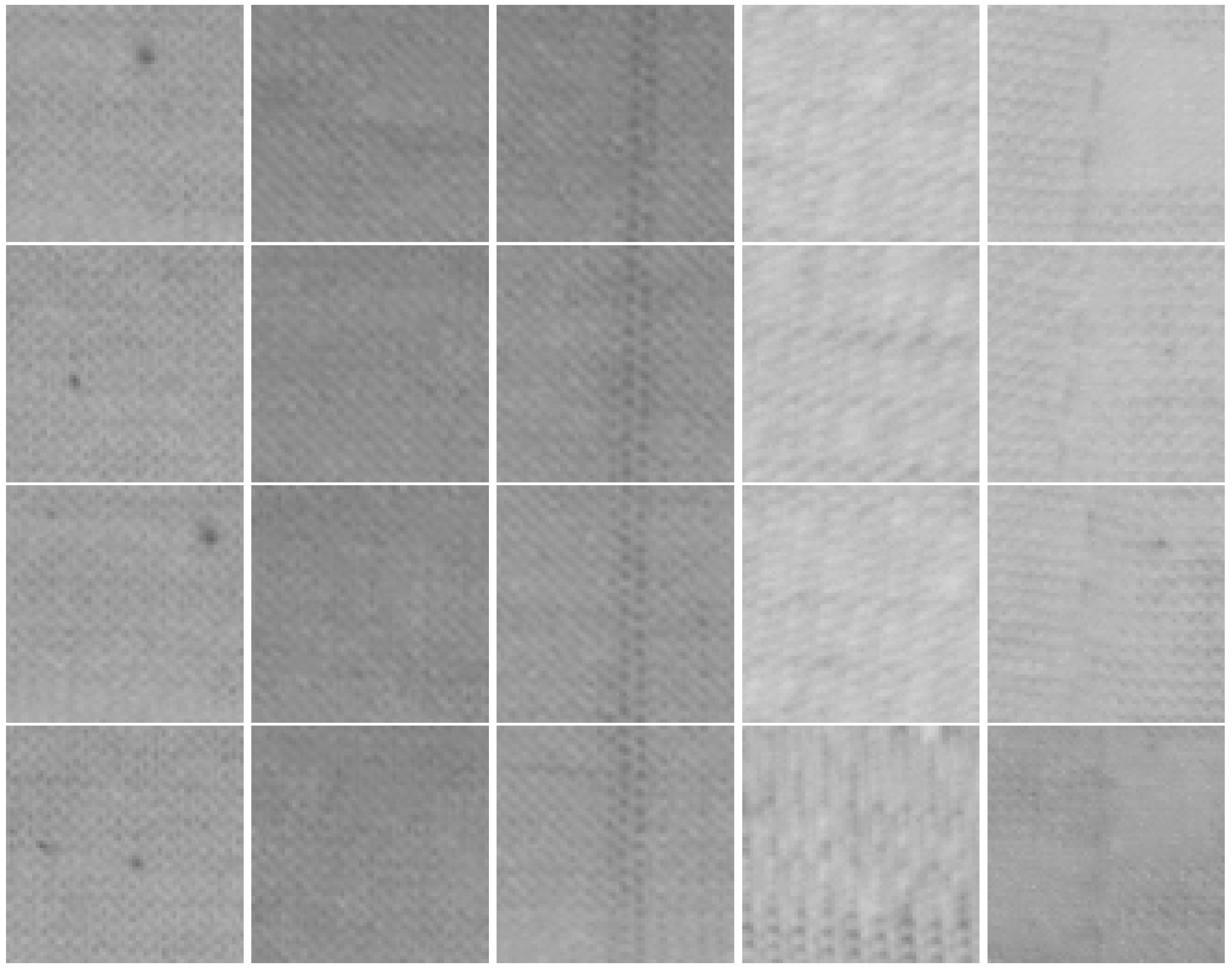
To build a robust dataset, it is important to gather a diverse set of fabric images that represent the full range of defects the model needs to detect. The dataset should include various defect types, severity levels, and orientations. Each defect type is organized into separate folders, each labeled with its corresponding defect code. The faulty fabric images contained within the dataset are depicted in Figure 2.
Augmenting the training dataset by applying various transformations to the images is crucial for helping the model generalize effectively and reducing overfitting. Common augmentations include rotation, flipping, scaling, brightness adjustment, and cropping. During the process of dividing images into 64 × 64 pixels, data augmentation can be applied by overlapping certain areas. Defects within the images are shifted and re-selected. Additionally, the dataset was further augmented by slightly altering the image scale by approximately 10%.
In many vision systems, particularly those employing machine learning algorithms, a large and diverse dataset is required for training. Data acquisition ensures that the system has access to a comprehensive set of examples from which it can learn, thus enhancing its ability to generalize and make accurate predictions.
The model’s performance on the validation set should be continuously evaluated, with adjustments made as new data are obtained from the machines. This may involve adding more fabric images or updating the data augmentation strategy. Once a well-prepared dataset for fabric defect detection is established, it can be used to train the model or fine-tune the parameters of other algorithms.

3. Curvature Algorithm

Curvature is an invariant descriptor associated with a curve, representing the rate at which the curve deviates from its tangent line. It is thus natural to relate curvatures in an image to the level lines. This algorithm calculates curvatures and other parameters, such as radius, at sub-pixel resolution. Following the application of an independent anti-aliasing filter to the evaluated lines and curves, smooth trajectories along the boundary are obtained [14,15,16].
In fabric defect detection, the integration of curvature analysis plays a critical role in enhancing the precision of the inspection process [17]. Initially, edge detection techniques, such as the Canny method, are applied to the raw fabric image [18]. This step is essential for highlighting boundaries and contour-like structures within the fabric. Next, a contouring algorithm is used to delineate and organize these accentuated edges, providing a foundation for further analysis [19]. The introduction of curvature analysis refines defect identification by examining the angles and radii of the extracted contours. Curvature analysis offers valuable insights into subtle variations in fabric patterns [20]. The combination of edge detection, contour algorithms, and curvature analysis creates a comprehensive approach, improving both the accuracy and reliability of fabric defect detection.

3.1. Discrete Curvature Algorithm

Discrete curvature is a mathematical approach used to measure the curvature in an image by employing discrete techniques. It calculates the change in direction of individual pixels and aggregates these changes to form a continuous curvature measurement. Traditional methods for calculating discrete curvatures have relied on finite difference schemes; however, these methods often produce spurious oscillations along horizontal and vertical lines due to their dependence on grid values.
Before applying the algorithm that utilizes these formulas, edge detection and contouring operations must first be performed. The contours derived from these processes are subsequently used to execute the discrete curvature function, which calculates the appropriate curvature values.
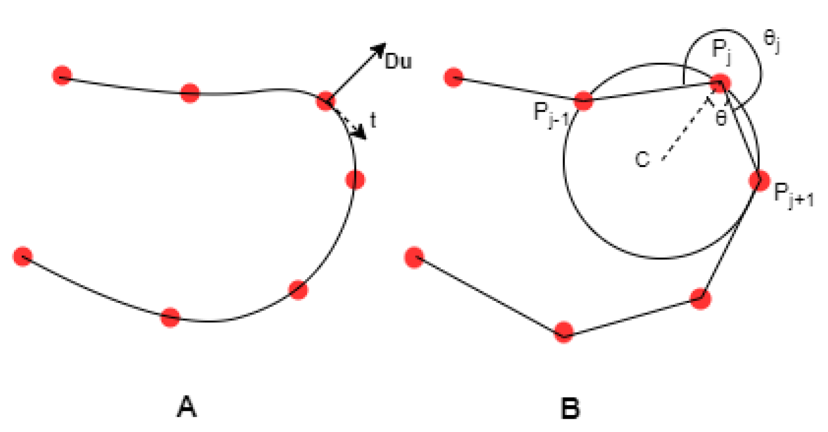
The methodology involves discretizing a continuous level line, where each level line is represented as a polygon defined by its ordered vertices. For simplicity, and to reduce dependence on specific variables, a level line is generally denoted as = P j ( x j , y j ) j = 0 , 1 , , N , with the condition that P 0 = P N . Here, each vertex P j represents a point in the plane with coordinates ( x j , y j ) . At any vertex P j , the curvature κ ( P j ) can be calculated as the inverse of the constrained radius. More precisely, for each j 0 , 1 , , N , three consecutive points, P j 1 , P j , and  P j + 1 , define a triangle. The radius r j of the circle inscribed in this triangle is then computed, yielding the (signed) discrete curvature  [14].
The (signed) discrete curvature at P j is given by the following:
K ( P j ) = ± 1 / r j .
The discrete curvature at point P j is given as follows:
K ( P j ) = 2 s i n θ j P j P j 1 = 2 s i n ( d e t ( P j P j 1 ) , P j P j + 1 ) P j 1 P j P j P j + 1 P j 1 P j + 1 .
where θ j ( P j P j 1 P j P j + 1 ) is the angle and the numerator of the right side contains the term.
d e t ( P j P j 1 P j P j + 1 ) = d e t ( x j 1 x j x j + 1 x j y j 1 y j y j + 1 y j ) .
The center of the circumscribed circle of the triangle is C and θ j = ( P j P j + 1 , P j C ) . Since point C is on two perpendicular bisectors, by the cosine theorem,
r j 2 = r j 2 + r + 2 2 r j 2 r + 2 c o s ( θ ) .
The distance between consecutive vertices P j and P j + 1 is denoted as r + = | P j P j + 1 | . This can be simplified as follows:
r j c o s ( θ ) = P j P j + 1 2 .
where r j is the radius of the inscribed circle, and  θ is the angle formed by the vertices. Additionally, the following relationship between the radii can be derived:
r j 2 = r j 2 + r 2 2 r j 2 r 2 cos ( θ + θ j ) ,
where r = | P j 1 P j | represents the distance between the previous pair of vertices, P j 1 and P j . Simplifying further, we have the following:
r j c o s ( θ + θ j ) = P j 1 P j 2 .
taken by eliminating r j between both equations and expanding the cosine of a sum, we obtain:
( r + c o s θ j r ) c o s ( θ ) = r + s i n ( θ j ) s i n ( θ ) .
Like this;
t a n ( θ ) = r + c o s θ j r r + s i n θ j .
When tan( θ ) is substituted into the formula below
1 | c o s ( θ ) | = 1 + t a n 2 ( θ ) = r + 2 r 2 2 r + r c o s ( θ j ) r + | s i n ( θ j ) | = P j P j + 1 r + | s i n ( θ j ) | .
If we combine the law of cosine with the last equation, we obtain
1 K ( P j ) = r j = ( P j 1 ) ( P j + 1 ) 2 | s i n ( θ j ) | .
The last equality of the proposition comes from the vector product property.
d e t ( P j P j 1 P j P j + 1 ) = r + r s i n ( θ j ) .
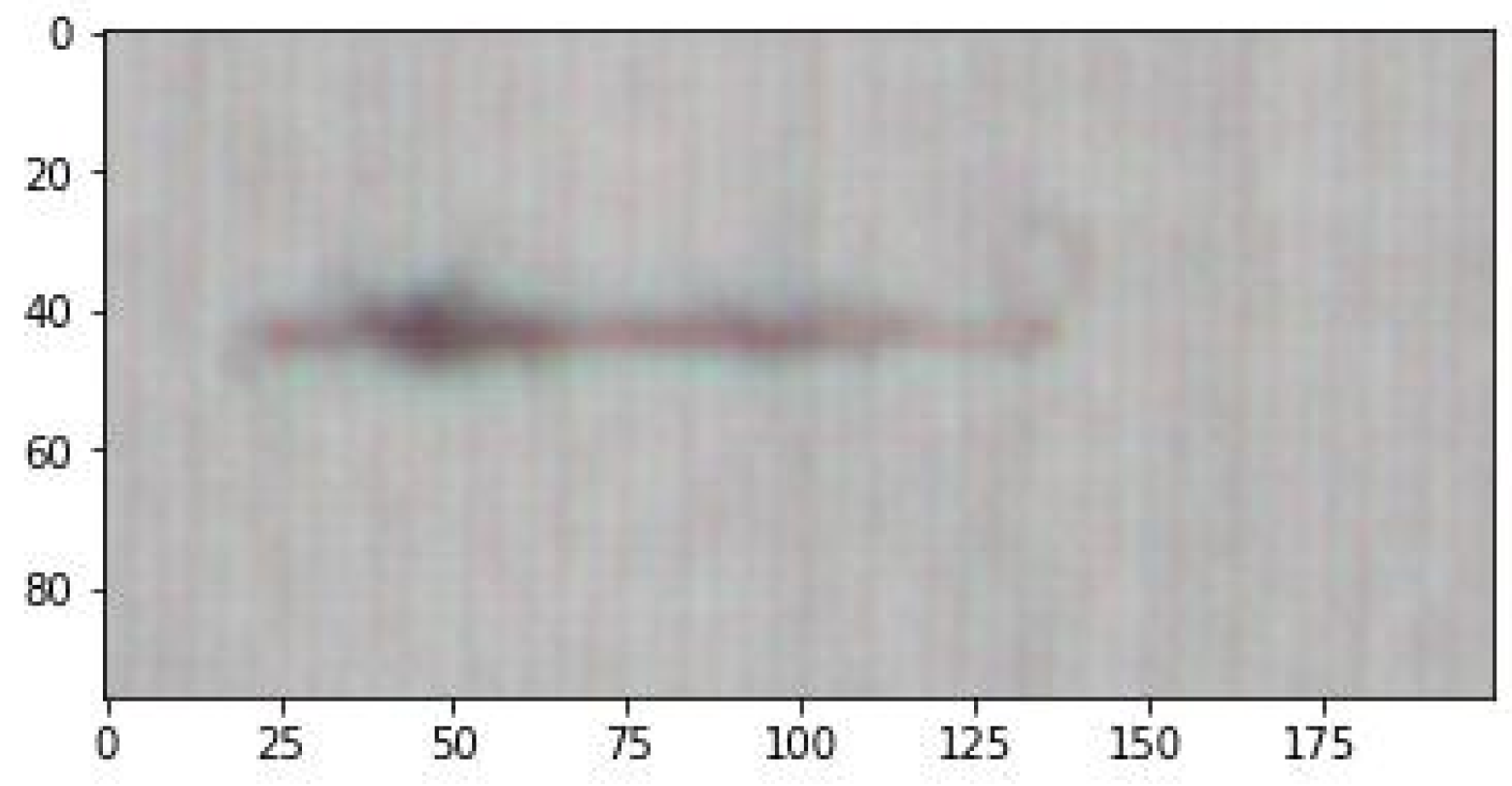
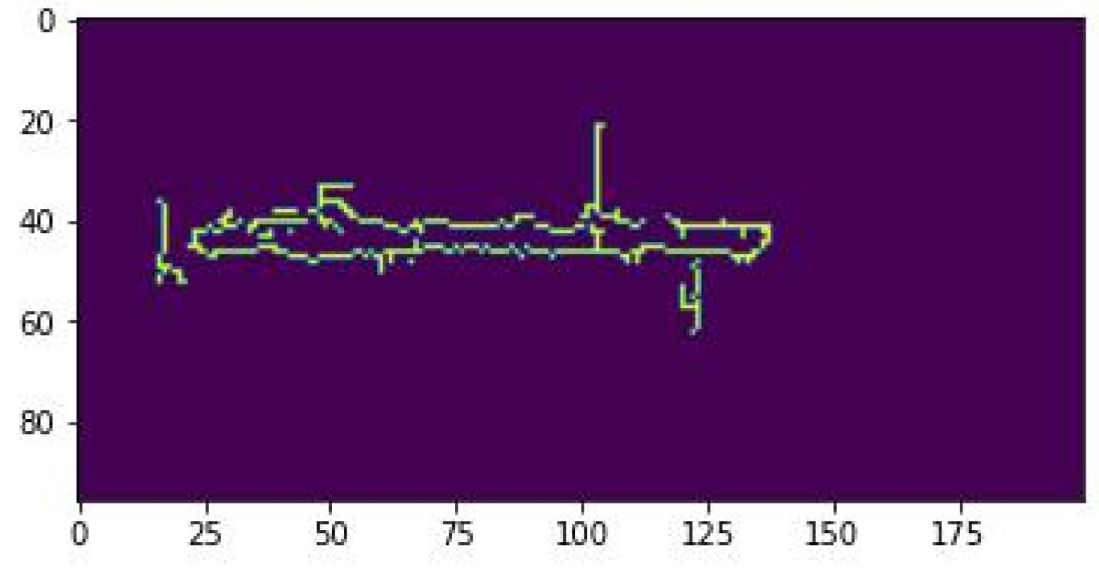
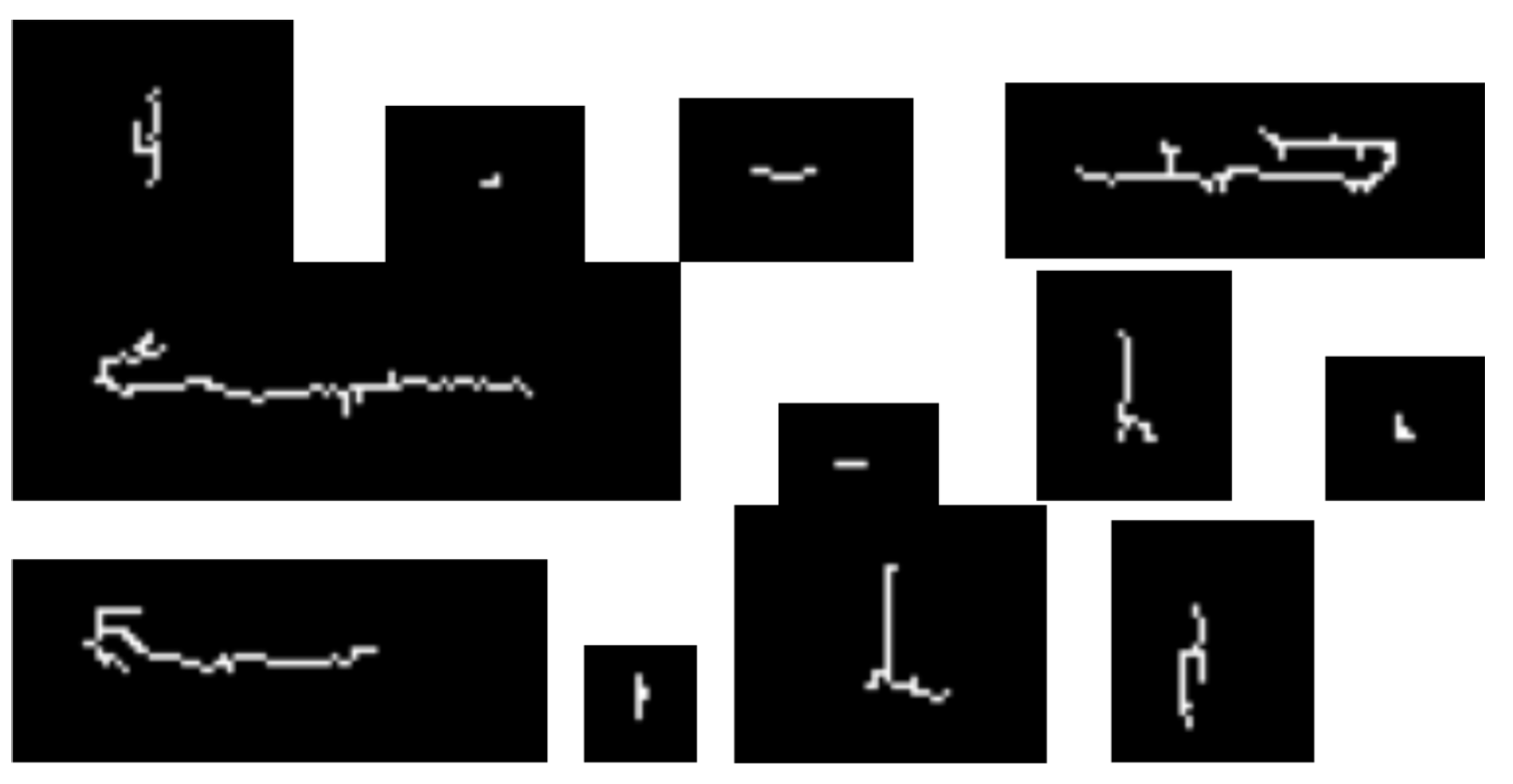
In the initial stage, the defective fabric image is captured using the proposed setup, as illustrated in Figure 3. As a pre-processing step, the Canny edge detection algorithm is applied, as depicted in Figure 4. The resulting edges are utilized as sub-contours within the contour algorithm. Following this, curvature values are computed using these sub-contours and 3-point structures within the discrete curvature function. The defect boundary is subsequently delineated by the contour segments, as shown in Figure 5.
After applying edge detection to identify defects in the fabric, the borders of these faults are extracted. These borders contain the characteristic parameters of the defects, such as the radius and external angle. The discrete curvature algorithm is employed to calculate these parameter values. By analyzing the specific ranges of radius and angle, the type of defect can be classified.
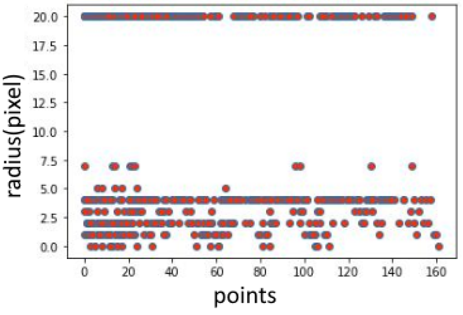
As illustrated in Figure 6B, each point along the edge is associated with a radius and an external angle relative to the generated circle. Once the edges are constructed on the sample image, the algorithm is applied to each point along the contours, and the results are presented graphically. The proposed algorithm computes the radius values for each point in the edge-detected images, as depicted in Figure 7.
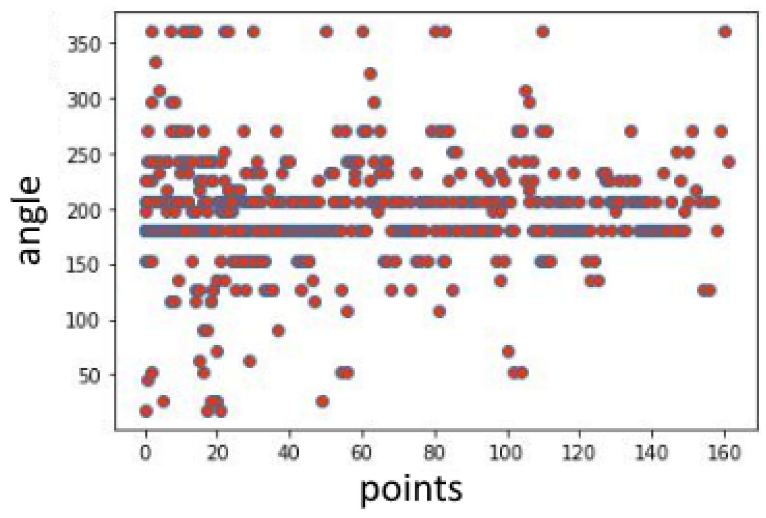
The exterior angle, θ j , graph is given in Figure 8.
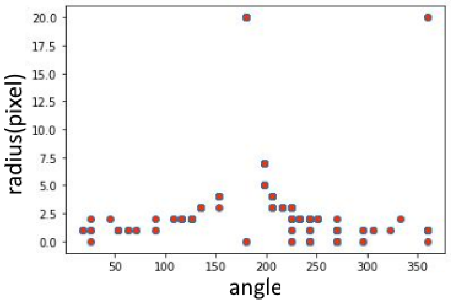
The graph of curvature radius vs exterior angle on the edge, θ j , is given in Figure 9.
During the construction of the confusion matrix, two classes, “faulty” and “non-faulty”, were defined, with the corresponding images saved in separate directories. Each data directory was enumerated, and all images were processed. The predicted class of each result was compared to the actual class, and based on this comparison, the confusion matrix was generated. Following the application of the curvature-based approach, the resulting confusion matrix is presented in Table 1.
The results of the standard discrete curvature algorithm were insufficient, leading to the development of a modified discrete curvature algorithm with a new computational approach.

3.2. Modified Discrete Curvature Algorithm

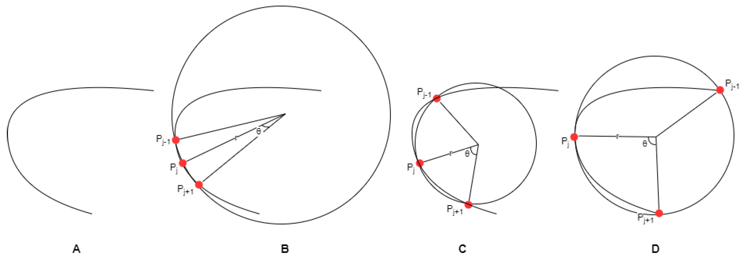
In the standard curvature algorithm, successive sets of three points are selected along the curve. However, this method resulted in excessively large radius values. To address this issue, we modified the algorithm by incorporating a geometric check of the curve to obtain more reasonable radius values. Specifically, it was proposed to examine the second derivative of the curve function to distinguish between concave geometry, where f ( x ) > 0 , and convex geometry, where f ( x ) > 0 .
Figure 10 illustrates the calculation of angle and radius values using the discrete curvature algorithm with a 3-point structure. Figure 10A presents a sample curve for evaluation. Figure 10B shows the traditional curvature method where points are selected in close succession, which leads to excessively large radius values and inaccurate angle calculations. In Figure 10C,D, alternative methods are depicted for achieving more accurate and optimal results.
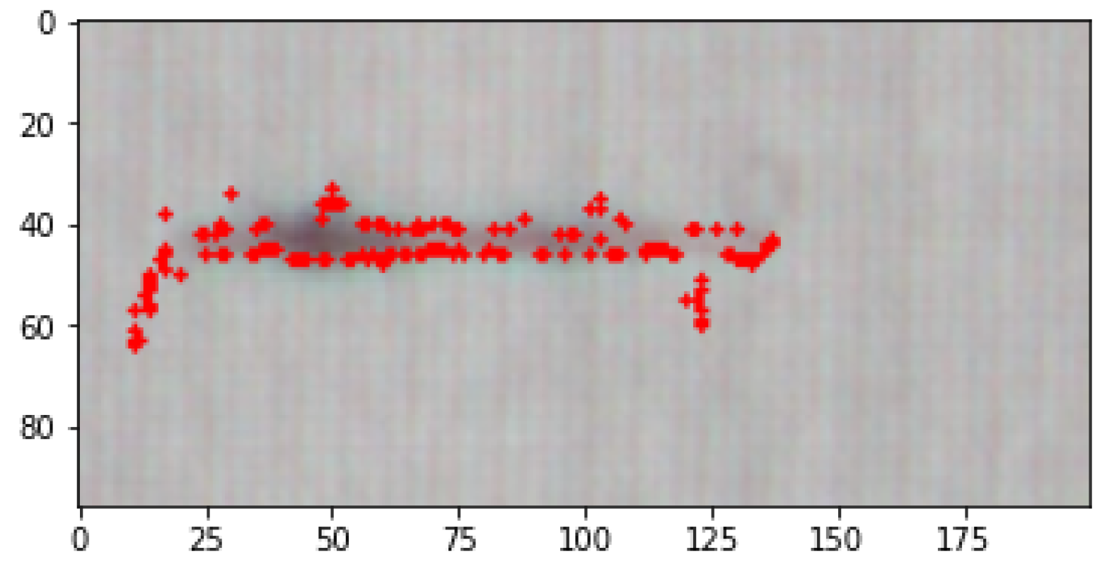
The new 3-point selection strategy maximizes the coverage area, as shown in Figure 10, thereby enabling more accurate curvature calculations. Additionally, the total number of points was significantly reduced, leading to faster processing. The detection result obtained by applying this method on contour pieces is shown in Figure 11.
The pseudo code of the described Modified Discrete Curvature Algorithm is presented Algorithm 1. The difference from Discrete Curvature can also be observed in the line titled Checking Convex or Concave.
Algorithm 1 Modified Discrete Curvature Algorithm
Require: image ( n × n ) n o n e m p t y
    if Filter selection type then
           f i l t e r e d i m a g e = f i l t e r ( i m a g e )
    end if
     c o n t o u r s f i n d C o n t o u r s ( f i l t e r e d i m a g e ) ▹ finding Countours
    while  N l e n ( c o u n t e r s ) do
         C I L i s t = D i s c r e a t e C u r v a t u r e ( c o u n t e r s ) ▹ return( r j , t h e t a , t h e t a j , k p j )
    end while
    while  m C I L i s t  do
        if  t h e t a j i s < 180  then▹ Checking convex or concave
             d i r c u r v = 1
        else if  t h e t a j i s > 180  then
             d i r c u r v = 2
        else if  t h e t a j i s = 180  then
             d i r c u r v = 3
        end if
        dircurv is changed append values to the C I L i s t e d g e
    end while
    while  m C I L i s t e d g e  do
        if  C I L i s t e d g e  is between  x 1 < r j < y 1 , a 1 < t h e t a j < b 1 t y p e 1  then
            defect type is hole or oil
        end if
        if  C I L i s t e d g e  is between  x 2 < r j < y 2 , a 2 < t h e t a j < b 2  then
            defect type is vertical or horizontal
        end if
    end while
The results demonstrate that the proposed method, utilizing the modified curvature algorithm, produces more accurate outcomes, as reflected in the confusion matrix in Table 2. This highlights the method’s potential application in defect detection. Consequently, further studies will be undertaken to advance and refine this approach.
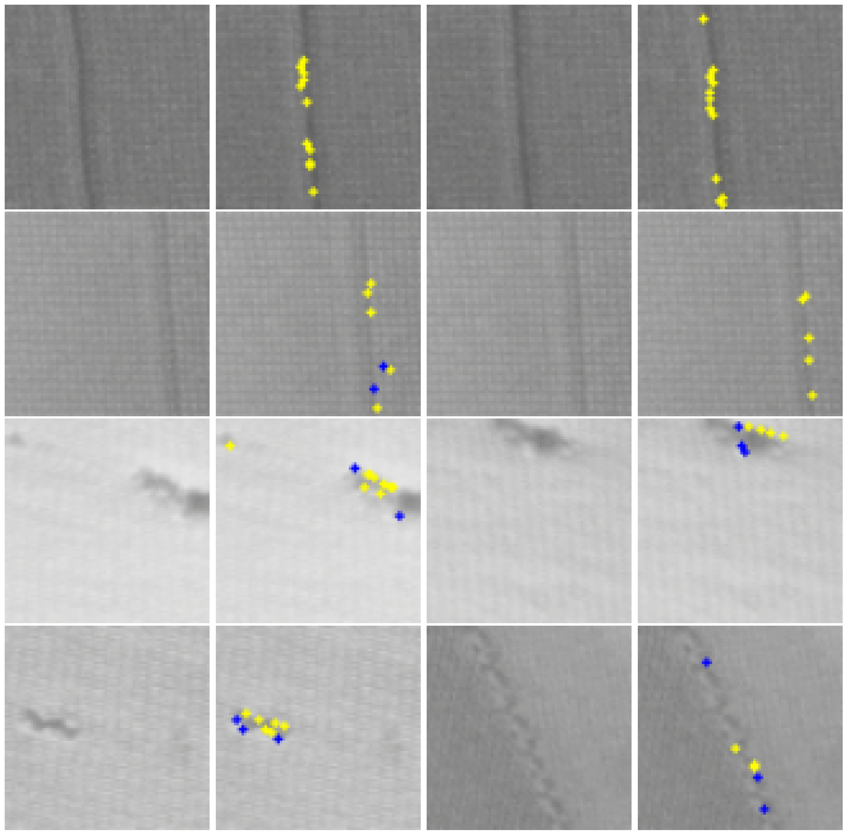
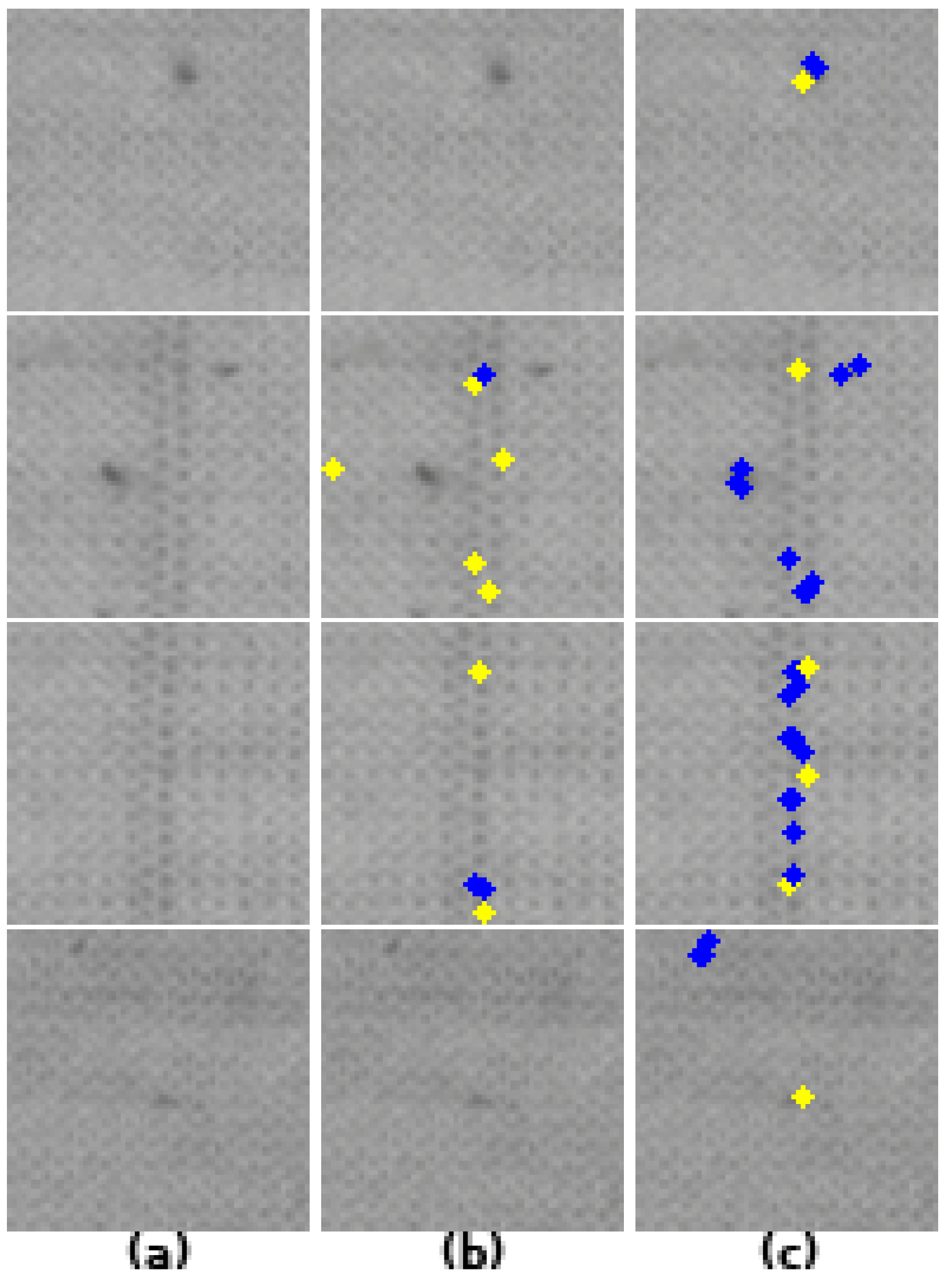
After the curvature algorithm was modified, the success rate increased significantly, as demonstrated by the confusion matrices. The results obtained by applying the MDCA on sample images are shown in Figure 12. This improvement can also be observed in the comparative analysis with the CA presented below, as seen in Figure 13.

4. Gabor Transform-Based Approach

The regular repeating texture of fabrics can be characterized by dominant spatial frequency and orientation signatures of the underlying textile pattern. Two-dimensional (2-D) Gabor filters have been successfully applied to the analysis of textured images, particularly those with distinct frequency and orientation properties, making them highly suitable for textile fabric defect detection applications [21,22].
The 2-D Gabor filters have demonstrated their effectiveness in a wide range of image analysis tasks. They are regarded as one of the most efficient and widely used tools for applications such as texture boundary detection, image segmentation, discrimination, and texture classification  [23]. Recently, these filters have also been employed in the analysis of raw textile fabrics  [24]. Texture analysis methods utilizing 2-D Gabor filters can be broadly divided into two categories: filter banks and individually tuned/matched filters.
The filter bank approach requires a large set of filters with predefined parameters to adequately cover the frequency plane, resulting in a correspondingly high-dimensional feature space  [25]. While this extensive filter bank can improve segmentation, it may also negatively affect the quality of classification and recognition  [26]. In contrast, tuned/matched Gabor filters address the limitations of the filter bank approach  [27]. The parameters of the optimized/tuned Gabor filter set are closely aligned with the textural features to be detected, making them particularly suitable for segmentation and classification tasks [28,29].
The pseudo code of the described Gabor Transform Algorithm is presented Algorithm 2.
Algorithm 2 Gabor Transform Algorithm
Require: image  ( n × n ) n o n e m p t y
     k e r n e l g e t G a b o r K e r n e l ( ( k s i z e , k s i z e ) , s i g m a , t h e t a , l a m d a , g a m m a , p h i )
    if Filter selection type then
         f i l t e r e d i m a g e = f i l t e r ( i m a g e )
    end if
     G a b o r i m a g e f i l t e r 2 D ( i m a g e , k e r n e l ) ▹ Gabor Transform Image
    while  ( n × n ) G a b o r T r a n s f o r m I m a g e ( )  do
        Sum the energy density of all pixels.▹ Calculate the energy density
    end while
    if Energy density is ≥ Threshold Energy then
        Image is defected
    end if
Gabor filters can also be utilized in conjunction with techniques such as the co-occurrence matrix and core principal component analysis (PCA) to detect fabric defects. These combined methods have successfully achieved high detection rates in online fabric inspection. The use of Gabor filters facilitates the extraction of features for various defect types, as defect classification is based on the specific filter types employed.
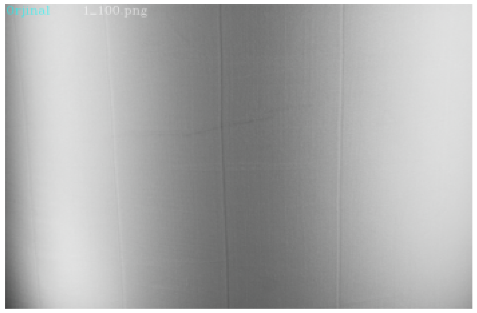
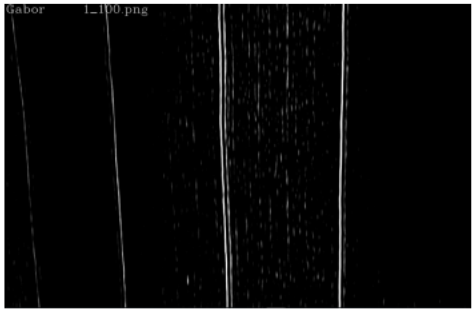
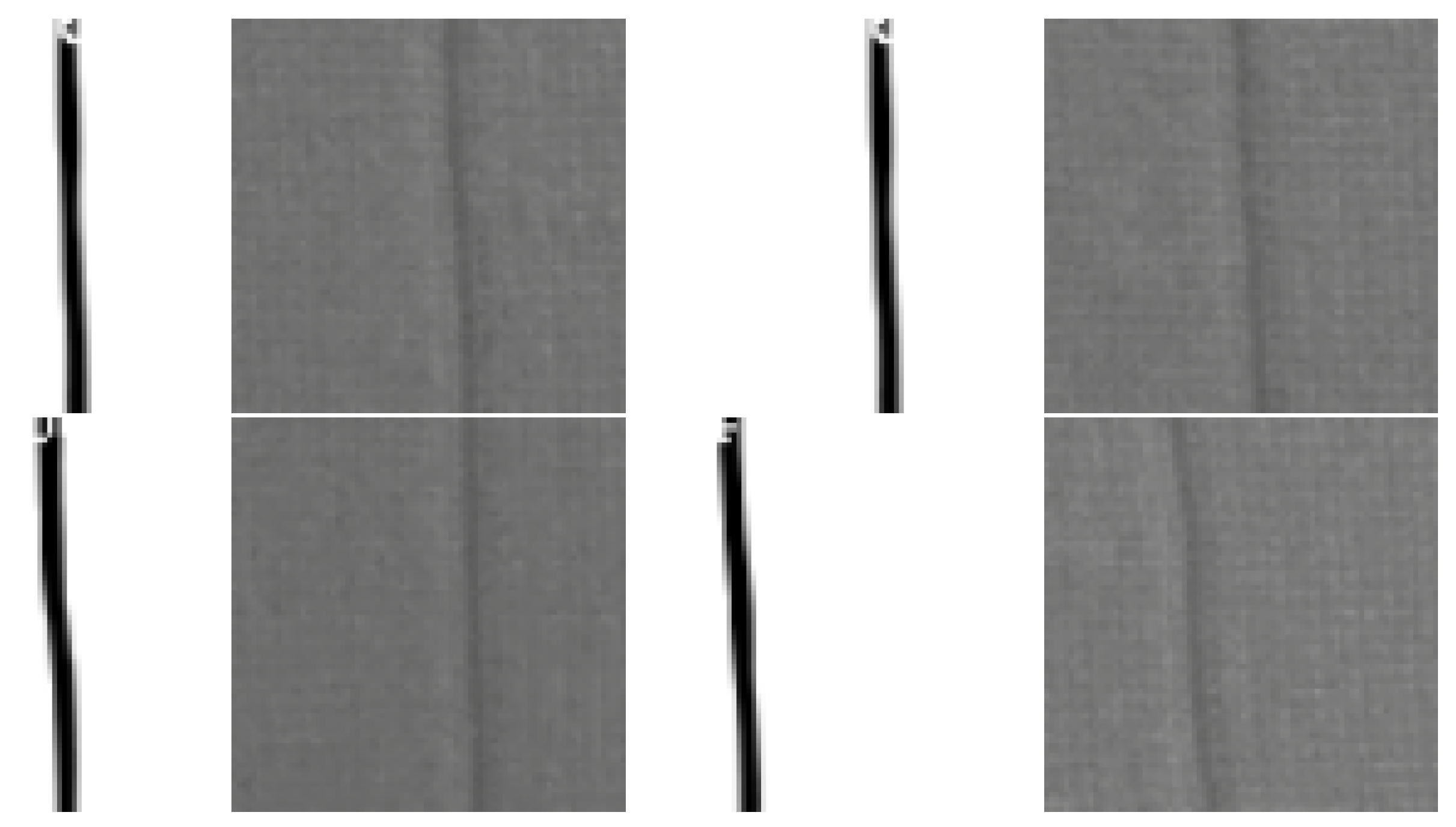
In this research, defective fabric images were captured using the experimental setup illustrated in Figure 14. Subsequently, Gabor filters were applied to these images, and regional energy densities were examined as a novel approach. The filtered image is shown in Figure 15. Regions with high energy density were identified as faults using our newly designed filter bank. To achieve a high detection accuracy, the filter parameters were optimized to align with the fabric texture. A confusion matrix was constructed based on the detection results, classifying images as either faulty or flawless, with a partial representation shown in Figure 16. The results obtained using this new approach are presented in Table 3.

5. Ablation Study on Deep Learning-Based Defect Detection

This section analyzes the performance of deep learning-based approaches for defect detection, focusing on the use of pre-trained CNN models and transfer learning. The aim is to compare traditional machine learning methods with state-of-the-art deep learning techniques in terms of accuracy, training efficiency, and robustness to challenging conditions. Traditional machine learning methods for defect detection are effective but often rely on manual feature extraction, which requires expert knowledge and limits the generalizability of these methods [30,31]. In recent years, convolutional neural networks (CNNs) have garnered increasing attention due to their ability to automatically extract features [32,33]. Designing a compact and efficient CNN model capable of capturing low-level features while detecting surface defects quickly and accurately is essential  [34].
One potential solution is to employ a pre-trained model as the backbone architecture and apply transfer learning or fine-tuning to adapt it to the specific task  [35]. Transfer learning or fine-tuning involves transferring parameters, such as weights and biases, from a previously trained model to a new model  [36]. This approach enables the development of high-performance models in a relatively short time  [37]. Moreover, pre-trained models, when trained on large datasets, can achieve high performance when applied to different datasets  [38]. Examples of pre-trained models include SqueezeNet, GoogLeNet, InceptionV3, and ResNet50V2 [39,40]. In test datasets containing various surface defects, such as those influenced by challenging conditions like strong diffuse illumination, camera noise, and motion blur, only a small number of training samples with defects are required to achieve highly accurate detection results [41,42,43,44,45].
The proposed model must satisfy real-time processing requirements and match the camera’s image acquisition rate (fps) [46]. The software used to process the captured images should be aligned with the hardware’s processing time  [47]. Given that defects may vary in size, ranging from small to medium, the model must be adapted to detect features at multiple scales. In the initial layers, smaller convolutional filters are applied to capture fine, detailed anomalies, while larger filters are employed in deeper layers to detect broader, more pronounced defects. Horizontal and vertical directional defects are more effectively captured by incorporating elongated, direction-sensitive filters in the early layers, enhancing the model’s sensitivity to distinct linear patterns. Additionally, the integration of residual blocks enables the construction of a deeper network, facilitating the learning of complex, multi-layered features while simultaneously improving the efficiency of error backpropagation, thus optimizing the overall learning process [48]. This model was designed to allow for a fair comparison with other methods while demonstrating comparable performance [49,50]. Experimental results confirm that the proposed method is simple, effective, and robust in detecting fabric surface defects.
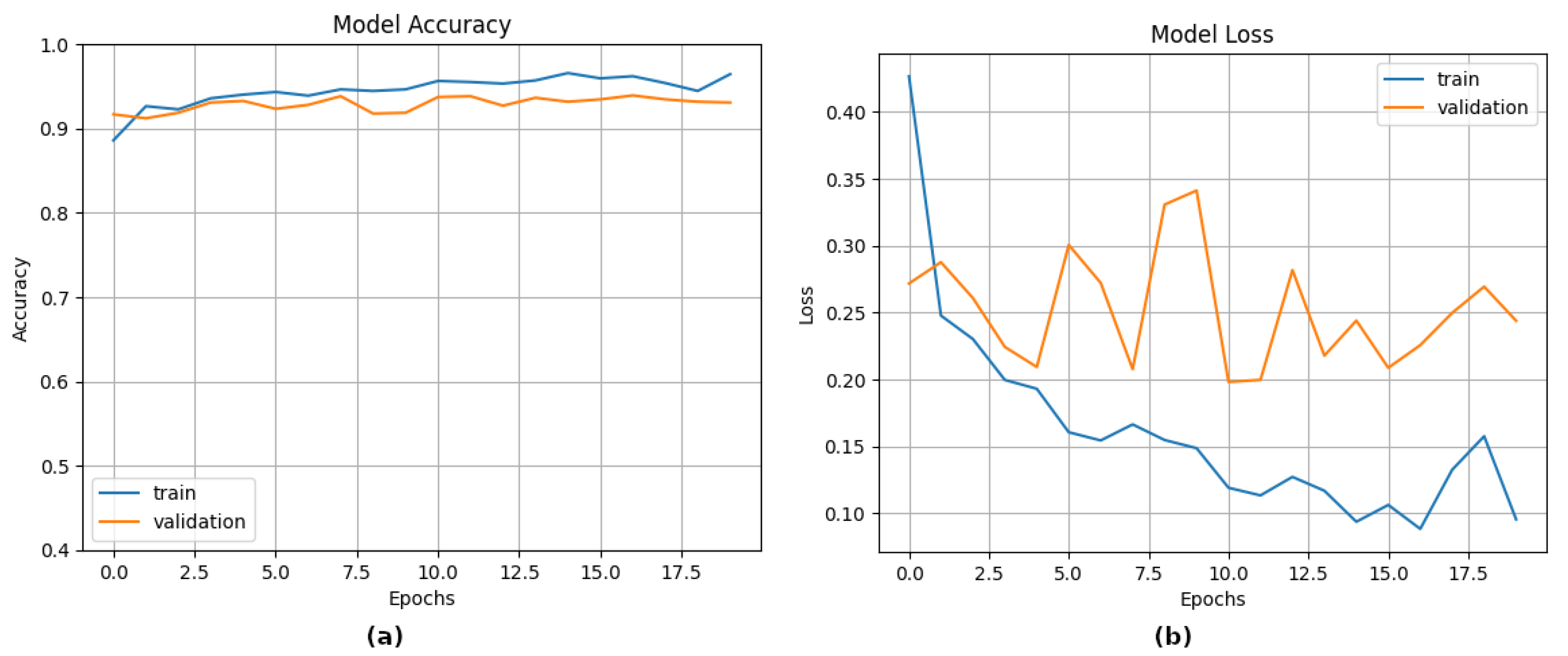
A batch size of 32 was selected to balance memory usage and training efficiency. Smaller batch sizes, like the one chosen, tend to allow more frequent updates to the model’s weights, which can lead to faster convergence, as discussed in  [51]. The model was trained for 20 epochs, which was found to be sufficient for the model to learn meaningful patterns from the data without overfitting. The number of epochs was determined experimentally, ensuring that the model had enough time to converge without training for too long, which could lead to diminishing returns and overfitting. The model accuracy over 20 epochs is presented in Figure 17a. During training, the train loss, representing the error in the training data, steadily decreased, indicating improved performance. The val loss, measuring the error on unseen validation data, was carefully monitored to prevent overfitting and ensure the model generalized well to new data. The changes in train loss and val loss over the course of training can be observed in Figure 17b.
For optimization, the Adam optimizer was selected due to its adaptive learning rate capabilities and overall efficiency in training deep learning models, as described by  [52]. Adam is known for its ability to converge quickly by adjusting the learning rate for each parameter dynamically, which makes it well-suited for complex models like the one used in this study. Additionally, the categorical cross-entropy loss function was used, as this is the standard loss function for multi-class classification problems  [53]. It calculates the difference between the true labels and the predicted probabilities output by the model, and minimizing this difference helps the model improve its predictions. Overall, these hyperparameters were chosen based on their effectiveness in training deep-learning models and were fine-tuned to maximize performance in fabric defect detection. The pseudo code of the described Deep Learning Based Algorithm is presented Algorithm 3.
Algorithm 3 Deep Learning Based Algorithm
Require: There must be images with all types and divided by different directory with class names and image ( n × n ) n o n e m p t y .
  Preparing The Data
   v a l _ d s = t f . k e r a s . p r e p r o c e s s i n g . i m a g e _ d a t a s e t _ f r o m _ d i r e c t o r y ( p a r a m e t e r s )
   c l a s s _ n a m e s = t r a i n _ d s . c l a s s _ n a m e s
  Training The Model
  model = Sequential()
  pretrained_model = tf.keras.applications.X()
  model.add(pretrained_model)
  # Add some layers of the pre-trained model
  # Modify a specific layer
  model.add(Flatten())
  model.add(Dense(512, activation = ’relu’))
  model.add(Dense(5, activation = ’softmax’))
  history = model.fit()
  Making Predictions
  pred = model.predict(image)
  print(pred)
The images captured from the test setup were classified as defective or non-defective using a pre-trained simple model, after which these images were visually inspected and used for model training [54]. Fabric defects were detected by the model trained with a CNN, and the areas with high error scores were marked and labeled [55]. Figure 18 and Figure 19 present the raw and processed images, respectively. Based on these results, a confusion matrix was constructed, as shown in Table 4 [56].

6. Result and Discussion

The images of defective fabrics were captured using an advanced camera-optic system. The identification algorithm was developed and tested using different approaches. Experimental results were analyzed, and the performance of various methods was evaluated. Defective fabrics collected from knitting factories were integrated into the in-house test setup, with the operating environment designed to simulate production sites. The captured images contained different physical defects, such as needle breakage, Lycra issues, and oil stains. The system classified the fabrics as either defective or non-defective, without specifying the type of fault. Subsequently, the confusion matrix and performance scores were generated for the different approaches.
The results for each type of defect are presented in Table 5 for all models. Based on these findings, it is possible to discern which model is more effective in identifying specific types of defects.
The experimental test results are summarized in Table 6, providing a comparison of accuracy and precision values.
Since the defects in the machine are 1 mm or larger, a minimum of 4 pixels must be captured within a 1 mm square area to detect the defect. When this requirement is calculated alongside the daily capacity of the machine, it results in 50–60 GB of data that must be processed and stored per day. Given the real-time study objective, the proposed discrete curvature algorithm is inferred to be more advantageous than learning-based algorithms in terms of the volume of data that needs to be processed and recorded.
Based on the test results for the faulty images, instead of storing 57,600 bytes of data for a 96 × 200 pixel image, it is more efficient to store 5100 bytes of extracted data from 638 points by considering the angle values, pixel positions, and radii. This approach significantly improves the compression rate and enhances real-time capability.
The discrete curvature algorithm proposed for faulty fabric detection was applied to faulty fabric images, and the results obtained through specific developments for this problem are presented. By calculating the degree of curvature for each point, the system determined whether the curvature was concave or convex, and an updated discrete curvature function was obtained through an intelligent selection algorithm. It has been demonstrated that this approach can be effectively used for defect detection by leveraging efficient external radius and angle values.
The Gabor transform achieves a high success rate in detecting vertical and horizontal defects with parameter settings specific to these types of faults. However, despite these successful results for vertical and horizontal defects, it does not yield satisfactory results for diagonal and other types of defects. Parameter adjustments are required to maintain performance across different fabric types.
Fabric defect detection using learning-based methods requires high computational performance and substantial training data compared to other approaches. The highest accuracy was achieved when pre-trained models were used. High-performance hardware is essential for local defect detection, and when these hardware requirements are met, the learning-based method achieves high success rates. Furthermore, different versions of YOLO were tested, and the results are presented in Table 7.
All calculations and tests indicate that hardware selection plays a critical role in achieving real-time defect detection. The processing times, provided in Table 8, were calculated using a Raspberry Pi 4. Subsequently, all tests were also conducted on a Jetson Nano, and their performances were compared. The NVIDIA Jetson Nano delivered superior performance, approaching real-time criteria. The learning-based method, executed on the GPU for a single image, takes approximately 110–130 ms. These results demonstrate that it is feasible to implement a near real-time embedded system.
The implemented system encountered several challenges, including overheating due to high illumination power, rapid LED switching issues, camera-LED synchronization problems, and assembly difficulties. The overheating issue was mitigated by improving the mechanical design and significantly reducing the on-time of the power LEDs. A custom-designed control board was developed to manage the lighting speed, enabling on/off switching and brightness control at millisecond intervals using Pulse Width Modulation (PWM). However, this flashing mechanism introduced synchronization problems with the camera, which were resolved through a software-based synchronization process. Furthermore, assembly-related challenges necessitated updates to the mechanical design and the development of new apparatuses to facilitate more efficient installation.

7. Conclusions

In conclusion, the modified discrete curvature method demonstrates strong potential, although it does not yet match the power of deep learning-based methods. This modified approach, combined with the newly applied techniques, shows promise in enhancing performance and accuracy while maintaining computational efficiency. The results from the Gabor transformation were also highly successful, largely due to parameter selection tailored to the faults, with most defects occurring horizontally and vertically. However, the success of these methods may vary with different fabric types. The modified discrete curvature method is particularly suited for local defect detection with minimal CPU usage and low power consumption.
In the future, the discrete curvature algorithm could be integrated with the Gabor approach to further improve accuracy and reduce execution time. Additionally, the system is expected to operate at higher frame rates (FPS) with enhanced accuracy, and future work will focus on developing noise detection algorithms to identify noise artifacts in the images. As a result, the developed system has the potential to serve not only the textile industry but also other sectors by detecting a wide range of surface defects.

Author Contributions

All authors contributed to the study conception and design. Material preparation, data collection and analysis were performed by [M.E.]. The first draft of the manuscript was written by [M.E.] and all authors commented on previous versions of the manuscript. Review and editing are conducted by [M.D.]. All authors read and approved the final manuscript.

Funding

This research received no external funding.

Data Availability Statement

Some sample images from the data-set are shown in Figure 2. The data-sets and software used during the current study are available from the corresponding author on reasonable request.

Conflicts of Interest

The authors declare that they have no financial interests or conflicts of interest related to this research.

Abbreviations

The following abbreviations are used in this manuscript:
CACurvature Algortihm
MDCAModified Curvature Algortihm
GTGabor Transform
CNNConvolutional Neural Network

References

  1. Hanbay, K.; Talu, M.F.; Özgüven, Ö.F. Fabric defect detection systems and methods—A systematic literature review. Optik 2016, 127, 11960–11973. [Google Scholar] [CrossRef]
  2. Kumar, A. 3-Computer vision-based fabric defect analysis and measurement. In Computer Technology for Textiles and Apparel; Hu, J., Ed.; Woodhead Publishing: Cambridge, UK, 2011; pp. 45–65. [Google Scholar] [CrossRef]
  3. Harwood, J.; Davis, G.; Wolfe, P. Automated Fabric Inspection Systems: Evaluation of Commercial Products. Text. Res. J. 2003, 73, 702–709. [Google Scholar] [CrossRef]
  4. Tsai, D.M.; Hsieh, C.Y. Automated Surface Inspection Using Gabor Filters. Int. J. Adv. Manuf. Technol. 1995, 10, 419–426. [Google Scholar] [CrossRef]
  5. Garbowski, T.; Maier, G.; Novati, G. On calibration of orthotropic elastic-plastic constitutive models for paper foils by biaxial tests and inverse analyses. Struct. Multidiscip. Optim. 2012, 46, 111–128. [Google Scholar] [CrossRef]
  6. Buljak, V.; Cocchetti, G.; Cornaggia, A.; Garbowski, T.; Maier, G.; Novati, G. Materials Mechanical Characterizations and Structural Diagnoses by Inverse Analyses. In Handbook of Damage Mechanics; Voyiadjis, G., Ed.; Springer: New York, NY, USA, 2015. [Google Scholar] [CrossRef]
  7. Asada, H.; Brady, M. The Curvature Primal Sketch. IEEE Trans. Pattern Anal. Mach. Intell. 1986, PAMI-8, 2–14. [Google Scholar] [CrossRef]
  8. Anandan, P.; Sabeenian, R.S. Fabric defect detection using Discrete Curvelet Transform. Procedia Comput. Sci. 2018, 133, 1056–1065. [Google Scholar] [CrossRef]
  9. Cao, F.; Moisan, L. Geometric Computation of Curvature Driven Plane Curve Evolutions. SIAM J. Numer. Anal. 2001, 39, 624–646. [Google Scholar] [CrossRef]
  10. Kimmel, R.; Malladi, R.; Sochen, N. Images as Embedded Maps and Minimal Surfaces: Movies, Color, and Volumetric Medical Images. Int. J. Comput. Vis. 1997, 39, 111–129. [Google Scholar] [CrossRef]
  11. Zhu, Y.; Er, M.J. Moment-Based Analysis of Closed Contours for Texture and Shape Classification. IEEE Trans. Syst. Man Cybern. Part Syst. Hum. 2000, 30, 525–533. [Google Scholar] [CrossRef]
  12. Li, H. Image Contour Extraction Method based on Computer Technology. In Proceedings of the 2015 4th National Conference on Electrical, Electronics and Computer Engineering, Xi’an, China, 12–13 December 2015; Atlantis Press: Paris, France, 2015; pp. 1185–1189. [Google Scholar] [CrossRef]
  13. Koenderink, J.J. The Structure of Images. Biol. Cybern. 1984, 50, 363–370. [Google Scholar] [CrossRef]
  14. Ciomaga, A.; Monasse, P.; Morel, J.-M. The Image Curvature Microscope: Accurate Curvature Computation at Subpixel Resolution. Image Process. Line 2017, 7, 197–217. [Google Scholar] [CrossRef]
  15. Tu, L.W. Differential Geometry: Connections, Curvature, and Characteristic Classes. In Graduate Texts in Mathematics; Springer: Cham, Switzerland, 2017; ISBN 978-3-319-55082-4. [Google Scholar]
  16. Sonka, M.; Hlavac, V.; Boyle, R. Image Processing, Analysis, and Machine Vision, 3rd ed.; Cengage Learning: Boston, MA, USA, 2008; pp. 223–230. [Google Scholar]
  17. Subrahmonia, J.D.; Lakshmanan, S.; Goldberg, M. Edge and curvature extraction for real-time road boundary detection. IEEE Trans. Veh. Technol. 1996, 45, 774–784. [Google Scholar]
  18. Canny, J. A computational approach to edge detection. IEEE Trans. Pattern Anal. Mach. Intell. 1986, 8, 679–698. [Google Scholar] [CrossRef] [PubMed]
  19. Suzuki, S.; Abe, K. Topological structural analysis of digital binary images by border following. Comput. Vision Graph. Image Process. 1985, 30, 32–46. [Google Scholar] [CrossRef]
  20. Papoulis, A. Probability, Random Variables, and Stochastic Processes, 4th ed.; McGraw-Hill: New York, NY, USA, 2000; pp. 315–318. [Google Scholar]
  21. Bovik, A.C.; Clark, M.; Geisler, W.S. Multichannel texture analysis using localized spatial filters. IEEE Trans. Pattern Anal. Mach. Intell. 1990, 12, 55–73. [Google Scholar] [CrossRef]
  22. Dunn, D.; Higgins, W.; Wakeley, J. Texture segmentation using 2-D Gabor elementary functions. IEEE Trans. Pattern Anal. Mach. Intell. 1994, 16, 130–149. [Google Scholar] [CrossRef]
  23. Jain, A.K.; Farrokhnia, F. Unsupervised texture segmentation using Gabor filters. Pattern Recognit. 1991, 24, 1167–1186. [Google Scholar] [CrossRef]
  24. Manjunath, B.S.; Ma, W.Y. Texture features for browsing and retrieval of image data. IEEE Trans. Pattern Anal. Mach. Intell. 1996, 18, 837–842. [Google Scholar] [CrossRef]
  25. Vautrot, P.; Bonnet, N.; Herbin, M. Comparative study of different spatial/spatial-frequency methods (Gabor filters, wavelets, wavelets packets) for texture segmentation/classification. In Proceedings of the 3rd IEEE International Conference on Image Processing, Lausanne, Switzerland, 19 September 1996; Volume 3, pp. 145–148. [Google Scholar] [CrossRef]
  26. Bigun, J.; du Buf, J.M.H. N-folded symmetries by complex moments in Gabor space and their application to unsupervised texture segmentation. IEEE Trans. Pattern Anal. Mach. Intell. 1994, 16, 80–87. [Google Scholar] [CrossRef]
  27. Teuner, A.; Pichler, O.; Hosticka, B.J. Unsupervised texture segmentation of images using tuned matched Gabor filters. IEEE Trans. Image Process. 1995, 4, 863–870. [Google Scholar] [CrossRef] [PubMed]
  28. Bodnarova, A.; Bennamoun, M.; Latham, S. Optimal Gabor filters for textile flaw detection. Pattern Recognit. 2002, 35, 2973–2991. [Google Scholar] [CrossRef]
  29. Clausi, D.A.; Jernigan, M.E. Designing Gabor filters for optimal texture separability. Pattern Recognit. 2000, 33, 1835–1849. [Google Scholar] [CrossRef]
  30. Liu, G. Surface Defect Detection Methods Based on Deep Learning: A Brief Review. In Proceedings of the 2020 2nd International Conference on Information Technology and Computer Application (ITCA), Guangzhou, China, 18–20 December 2020; pp. 200–203. [Google Scholar] [CrossRef]
  31. Zhang, Y.; Li, G.; Yang, J.; Wei, X. A review of machine learning-based defect detection methods. J. Manuf. Process. 2021, 66, 481–495. [Google Scholar] [CrossRef]
  32. Abbineni, J.; Thalluri, O. Software Defect Detection Using Machine Learning Techniques. In Proceedings of the 2018 2nd International Conference on Trends in Electronics and Informatics (ICOEI), Tirunelveli, India, 11–12 May 2018; pp. 471–475. [Google Scholar] [CrossRef]
  33. LeCun, Y.; Bengio, Y.; Hinton, G. Deep learning. Nature 2015, 521, 436–444. [Google Scholar] [CrossRef]
  34. Krizhevsky, A.; Sutskever, I.; Hinton, G.E. ImageNet classification with deep convolutional neural networks. In Advances in Neural Information Processing Systems; Curran Associates, Inc.: New York, NY, USA, 2012; pp. 1097–1105. [Google Scholar]
  35. Pan, S.J.; Yang, Q. A survey on transfer learning. IEEE Trans. Knowl. Data Eng. 2010, 22, 1345–1359. [Google Scholar] [CrossRef]
  36. Yosinski, J.; Clune, J.; Bengio, Y.; Lipson, H. How transferable are features in deep neural networks? In Advances in Neural Information Processing Systems; Curran Associates, Inc.: New York, NY, USA, 2014; pp. 3320–3328. [Google Scholar]
  37. Howard, J.; Ruder, S. Universal language model fine-tuning for text classification. In Proceedings of the 56th Annual Meeting of the Association for Computational Linguistics; Association for Computational Linguistics: Stroudsburg, PA, USA, 2018; pp. 328–339. [Google Scholar]
  38. Keshavan, M.S.; Janik, P. Transfer learning for improving performance of deep learning models in medical image analysis. J. Med. Imaging 2019, 6, 041201. [Google Scholar]
  39. Chen, Y.; Ding, Y.; Zhao, F.; Zhang, E.; Wu, Z.; Shao, L. Surface Defect Detection Methods for Industrial Products: A Review. Appl. Sci. 2021, 11, 7657. [Google Scholar] [CrossRef]
  40. Iandola, F.N.; Han, S.; Moskewicz, M.W.; Ashraf, K.; Dally, W.J.; Keutzer, K. SqueezeNet: AlexNet-level accuracy with 50x fewer parameters and <0.5 MB model size. arXiv 2016, arXiv:1602.07360. [Google Scholar]
  41. Chen, M.; Yu, L.; Zhi, C.; Sun, R.; Zhu, S.; Gao, Z.; Ke, Z.; Zhu, M.; Zhang, Y. Improved faster R-CNN for fabric defect detection based on Gabor filter with Genetic Algorithm optimization. Comput. Ind. 2022, 134, 103551. [Google Scholar] [CrossRef]
  42. Yu, W.; Lai, D.; Liu, H.; Li, Z. Research on CNN Algorithm for Monochromatic Fabric Defect Detection. In Proceedings of the 2021 6th International Conference on Image, Vision and Computing (ICIVC), Qingdao, China, 23–25 July 2021; pp. 20–25. [Google Scholar] [CrossRef]
  43. Liu, Q.; Wang, C.; Li, Y.; Gao, M.; Li, J. A Fabric Defect Detection Method Based on Deep Learning. IEEE Access 2022, 10, 4284–4296. [Google Scholar] [CrossRef]
  44. Lee, Y.J.; Grauman, K. Learning the easy things first: Self-paced visual category discovery. In Proceedings of the IEEE Conference on Computer Vision and Pattern Recognition, Colorado Springs, CO, USA, 20–25 June 2011; pp. 1721–1728. [Google Scholar] [CrossRef]
  45. Wei, Y.; Sun, Q.; Wang, L.; Liu, C. Few-shot learning for surface defect classification. IEEE Access 2020, 8, 32728–32736. [Google Scholar]
  46. Redmon, J.; Farhadi, A. YOLOv3: An incremental improvement. arXiv 2018, arXiv:1804.02767. [Google Scholar]
  47. He, K.; Zhang, X.; Ren, S.; Sun, J. Deep residual learning for image recognition. In Proceedings of the IEEE Conference on Computer Vision and Pattern Recognition, Las Vegas, NV, USA, 27–30 June 2016; pp. 770–778. [Google Scholar] [CrossRef]
  48. Simonyan, K.; Zisserman, A. Very deep convolutional networks for large-scale image recognition. arXiv 2014, arXiv:1409.1556. [Google Scholar]
  49. Huang, G.; Liu, Z.; Van Der Maaten, L.; Weinberger, K.Q. Densely connected convolutional networks. In Proceedings of the IEEE Conference on Computer Vision and Pattern Recognition, Honolulu, HI, USA, 21–26 July 2017; pp. 4700–4708. [Google Scholar] [CrossRef]
  50. Liu, S.; Jiang, X.; Yang, J.; Chen, B. A novel defect detection method based on feature extraction and recognition. Pattern Recognit. Lett. 2019, 119, 158–165. [Google Scholar] [CrossRef]
  51. Zhang, Y.; Wallace, B. A Sensitivity Analysis of (and Practitioners’ Guide to) Convolutional Neural Networks for Sentence Classification. IEEE Trans. Pattern Anal. Mach. Intell. 2015, 37, 397–409. [Google Scholar]
  52. Kingma, D.P.; Ba, J. Adam: A Method for Stochastic Optimization. In Proceedings of the International Conference on Learning Representations (ICLR), San Diego, CA, USA, 7–9 May 2015. [Google Scholar]
  53. Goodfellow, I.; Bengio, Y.; Courville, A. Deep Learning; MIT Press: Cambridge, MA, USA, 2016. [Google Scholar]
  54. He, Z.; Shao, H.; Chen, X. A deep learning-based approach for defect detection in manufacturing. J. Intell. Manuf. 2020, 31, 399–411. [Google Scholar]
  55. Szegedy, C.; Vanhoucke, V.; Ioffe, S.; Shlens, J.; Wojna, Z. Rethinking the inception architecture for computer vision. In Proceedings of the IEEE Conference on Computer Vision and Pattern Recognition, Las Vegas, NV, USA, 27–30 June 2016; pp. 2818–2826. [Google Scholar] [CrossRef]
  56. Grandini, M.; Bagli, E.; Visani, G. Metrics for multi-class classification: An overview. arXiv 2020, arXiv:2008.05756. [Google Scholar]
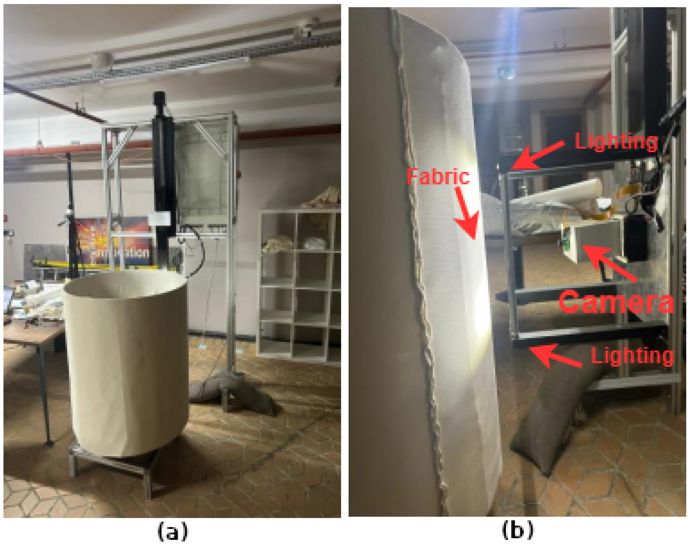
Figure 1. (a) Experimental Setup. (b) Close-Up View of Experimental Setup.
Algorithms 17 00506 g001
Figure 2. Defect data-set type hole, none, needle break, lycra, may (left to right).
Algorithms 17 00506 g002
Figure 3. Fabric with simple defect.
Algorithms 17 00506 g003
Figure 4. Fabric image with Canny edge detector.
Algorithms 17 00506 g004
Figure 5. Contour Pieces.
Algorithms 17 00506 g005
Figure 6. (A) Standard curve with points. (B) Calculation of discreate curvature.
Algorithms 17 00506 g006
Figure 7. Curvature radius values.
Algorithms 17 00506 g007
Figure 8. Exterior angle values.
Algorithms 17 00506 g008
Figure 9. Curvature radius vs exterior angle.
Algorithms 17 00506 g009
Figure 10. (A) Sample Curve, (B) Standard Curvature, (C) Optimized Curvature, (D) Efficient Curvature.
Algorithms 17 00506 g010
Figure 11. Defect detection with modified discrete curvature function.
Algorithms 17 00506 g011
Figure 12. MDCA Sample Fabric (left side) detected defects. (rigth side).
Algorithms 17 00506 g012
Figure 13. Comparision CA and MDCA algorithms (a) original (b) CA (c) MDCA.
Algorithms 17 00506 g013
Figure 14. Fabric image captured on experimental setup.
Algorithms 17 00506 g014
Figure 15. Gabor filter on fabric with defect.
Algorithms 17 00506 g015
Figure 16. Gabor filter on local fabric image.
Algorithms 17 00506 g016
Figure 17. (a) model accuracy, (b) model loss.
Algorithms 17 00506 g017
Figure 18. Fabric image dataset with defects.
Algorithms 17 00506 g018
Figure 19. Fabric defect detection and label with Cnn.
Algorithms 17 00506 g019
Table 1. Discrete Curvature Confusion Matrix.
Predicted
non-faultyfaulty
Actualnon-faulty50102152
faulty522274
102124226
Table 2. Modified Discrete Curvature Confusion Matrix.
Predicted
non-faultyfaulty
Actualnon-faulty10844152
faulty66874
114112226
Table 3. Gabor Transform Confusion Matrix.
Predicted
non-faultyfaulty
Actualnon-faulty13220152
faulty17374
13393226
Table 4. CNN Confusion Matrix.
Predicted
non-faultyfaulty
Actualnon-faulty1457152
faulty37174
17578226
Table 5. Defect Success Rate: CA (Curvature Algorithm), MDCA (Modified Curvature Algorithm), GT (Gabor Transform), CNN (Convolutional Neural Network).
Defect TypeHoleNeedle BreakMayLycraOil
CA0.420.290.270.320.40
MDCA0.780.820.740.810.60
GT0.810.990.990.850.78
CNN0.960.980.980.850.95
Table 6. Defect Detection Rate: CA (Curvature Algorithm), MDCA (Modified Curvature Algorithm), GT (Gabor Transform), CNN (Convolutional Neural Network).
ModelAccF1PrecisionRecallProcess Time
CA0.320.390.560.29203 ms
MDCA0.780.820.740.92295 ms
GT0.910.940.890.99110 ms
CNN0.960.960.960.961800 ms
Table 7. Comparision of Other Algorithms Yolov5, Yolov8n, Yolov8 TensorRT.
ModelYolov5Yolov8nYolov8 TensorRT
Inference time (min|max)172 ms|180 ms81.4 ms|81.9 ms65.6 ms|66.2 ms
mAP500.8460.85760.896
mAP50-950.5910.60.622
precision0.8140.870.866
recall0.8020.840.859
GFLOPs15.88.2078.2
parameters7,034,3983,013,3833,013,383
Table 8. Hardware Comparison of Algorithms CA (Curvature Algorithm), MDCA (Modified Curvature Algorithm), GT (Gabor Transform), CNN (Convolutional Neural Network).
ModelRPI4 CPUJetson Nano CPUJetson Nano GPU Acc.
CA4.9 fps5.5 fps-
MDCA3.38 fps3.8 fps-
GT9.1 fps10.2 fps-
CNN<1 fps1 fps8.33 fps
Disclaimer/Publisher’s Note: The statements, opinions and data contained in all publications are solely those of the individual author(s) and contributor(s) and not of MDPI and/or the editor(s). MDPI and/or the editor(s) disclaim responsibility for any injury to people or property resulting from any ideas, methods, instructions or products referred to in the content.