Local Convergence Study for an Iterative Scheme with a High Order of Convergence

Abstract

In this paper, we address a key issue in Numerical Functional Analysis: to perform the local convergence analysis of a fourth order of convergence iterative method in Banach spaces, examining conditions on the operator and its derivatives near the solution to ensure convergence. Moreover, this approach provides a local convergence ball, within which initial estimates lead to guaranteed convergence with details about the radii of domain of convergence and estimates on error bounds. Next, we perform a comparative study of the Computational Efficiency Index ($CEI$) between the analyzed scheme and some known iterative methods of fourth order of convergence. Our ultimate goal is to use these theoretical findings to address practical problems in engineering and technology.

1. Introduction

A significant issue in Numerical Functional Analysis is problem-solving in science and engineering using mathematical modeling techniques. A specific problem can be modeled, under certain conditions, as a nonlinear equation in a Banach space.

Let $X,Y$ be Banach spaces, D an open convex subset of X, and $\mathcal{T}$ a nonlinear operator, $\mathcal{T}:D\subseteq X\to Y$. The primary focus in studying an iterative method is to find the closest approximation to the solution of the equation $\mathcal{T}\left(x\right)=0$. However, it is crucial to ensure that the selected iterative method indeed converges to this approximation. To achieve both convergence and accurate results for the scheme, we can perform studies aimed at the necessary conditions that must be verified by the solution $x^{*}$, the initial value $x_0$, or the operator within the framework of the iterative method.

In Banach spaces, a convergence study can be approached from two perspectives: considering the neighborhood of the solution (referred to as local convergence analysis) or focusing on the initial estimates and the domain (known as semilocal convergence analysis). When we analyze local convergence (see [1,2]), conditions are applied on the operators and their respective derivatives at the solution $x^{*}$. In consequence, we obtain the local convergence ball, centered in the solution and with radius r: $B(x^{*},r)$. The elements contained within this ball are possible initial estimates which guarantee convergence, meaning that they are suitable initial points for the scheme to work or for which the sequence of iterates converges to the solution of the problem. Additionally, an error bound is established.

Local convergence analysis plays a significant role in understanding the behavior, efficiency, and reliability of an iterative method. This analysis provides detailed information about how fast an iterative method converges to a solution given an initial estimate. Moreover, through local convergence analysis we are able to identify the conditions under which an iterative method will converge to a solution, concerning initial estimate proximity and smoothness conditions. This analysis often provides error bounds, showing how the error decreases in each iteration, which helps in determining how accurate the current approximation is. In summary, local convergence analysis helps in choosing the right method, refining existing methods, and understanding their behavior under realistic conditions.

Local convergence analysis is essential in science and engineering for guaranteeing the accuracy, efficiency, stability, and adaptability of iterative methods used to solve complex real-world problems. Whether optimizing designs, conducting scientific simulations, solving nonlinear equations, or managing large-scale data, understanding the local convergence properties of an iterative scheme is necessary to achieve reliable and efficient solutions. For example, in Computational Fluid Dynamics (CFD), where simulations of airflow around objects may engage a large number of variables, fast local convergence can save considerable computational cost and make the process feasible. In molecular dynamics, iterative methods are used to study complex systems and the efficiency provided by a local convergence analysis can allow more detailed and expansive simulations. In mechanical engineering, solving the analysis of material deformations often requires iterative methods and local convergence analysis ensures these methods can handle the complexities of the system. In physics and chemistry, where iterative methods are used to solve quantum mechanical equations, local convergence analysis helps ensure accurate energy levels and wave functions are obtained. Computer-Assisted Diagnostic (CAD) systems rely heavily on various computational models and algorithms. These models often use iterative methods to solve complex mathematical problems (such as nonlinear equations, optimization tasks, and machine learning model training) and local convergence analysis is essential in ensuring the accuracy, efficiency, robustness, and adaptability of iterative methods used in CAD systems.

Several studies [2,3] have explored, for some iterative methods, local convergence under various continuity conditions. For instance, Argyros in [4], for the modified Newton’s method for multiple zeros, provides an estimate for the convergence radius, assuming the function meets Hölder and center-Hölder continuity conditions. This result is further refined by Zhou et al. in [5]. Bi et al. in [6] studied third-order methods, and they established local convergence using divided differences and its properties. Behl et al. (see [7]) used Taylor’s expansions to establish a new set of bounds in order to ensure convergence. Zhou and Song (see [8]) also employed Taylor’s expansions to analyze the local convergence of Osada’s method, but considering that the derivative verifies the center-Hölder continuity condition. In addition, Singh et al. [9] examined, for a fifth-order iterative scheme, both the local and semilocal convergence under Hölder continuity conditions.

In the semilocal convergence analysis, certain conditions are placed both on the operators and their respective derivatives at $x_0$ (the initial estimate), and iterations are then carried out. This leads to results such as the existence of the solution, its uniqueness, a priori error bound, the R-order of convergence of the scheme, and the ascertainment of the convergence region where the operator $\mathcal{T}$ is defined. In this work, we will focus on local convergence analysis. Some elements of this study are shown in [10].

This paper presents an iterative method along with its local convergence analysis for solving the nonlinear equation $\mathcal{T}\left(x\right)=0$, which has a solution $x^{*}$. Consider the (fourth-order) family of iterative schemes studied in [11], defined for $k=0,1,2,\dots$ by:

$$\begin{array}{cc}\hfill & y_k=x_k-{\displaystyle \frac{2}{3}}{\mathcal{T}}^{\prime }{\left(x_k\right)}^{-1}\mathcal{T}\left(x_k\right)\hfill \\ \hfill & x_{k+1}=x_k-\left[\left({\displaystyle \frac{5}{8}}-\alpha \right)+\alpha {\mathcal{T}}^{\prime }{\left(y_k\right)}^{-1}{\mathcal{T}}^{\prime }\left(x_k\right)+{\displaystyle \frac{\alpha }{3}}{\mathcal{T}}^{\prime }{\left(x_k\right)}^{-1}{\mathcal{T}}^{\prime }\left(y_k\right)\right.\hfill \\ \hfill & \left.+\left({\displaystyle \frac{3}{8}}-{\displaystyle \frac{\alpha }{3}}\right){\left({\mathcal{T}}^{\prime }{\left(y_k\right)}^{-1}{\mathcal{T}}^{\prime }\left(x_k\right)\right)}^2\right]{\mathcal{T}}^{\prime }{\left(x_k\right)}^{-1}\mathcal{T}\left(x_k\right).\hfill \end{array}$$

(1)

where $\alpha \in \mathbb{C}$ is a parameter and $x_0$ is the initial estimate.

In order to approximate the solution of the nonlinear equation $\mathcal{T}\left(x\right)=0$, it is assumed that the derivative ${\mathcal{T}}^{\prime }\left(x\right)$ exists in a neighborhood of the solution $x^{*}$ and that ${\mathcal{T}}^{\prime }{\left(x^{*}\right)}^{-1}\in \mathcal{L}(Y,X)$, where $\mathcal{L}(Y,X)$ is the set of bounded linear operators mapping from Y to X.

In the following sections, this paper addresses these topics: a local convergence analysis is presented in Section 2. In Section 3, we undertake a computational efficiency study of the new method and compare it with other existing schemes. Section 4 includes several numerical examples in order to validate the theoretical results. Concluding observations are summarized in Section 5.

2. Local Convergence Analysis

In this section, we provide the local convergence analysis for scheme (1). Let $\overline{B}(x^{*},r)$ and $B(x^{*},r)$ represent the closed and open balls, respectively, in Banach space X, centered in $x^{*}$ (the solution) with radius $r>0$. In order to develop a local convergence study, certain conditions are applied on operators $\left(\mathcal{T},{\mathcal{T}}^{\prime }\right)$ in $x^{*}$, which is presumed to exist. Hence, we consider, for real numbers $L_0>0,L>0$ and for all $x,y\in D$, the conditions listed below:

(C₁)

$\mathcal{T}\left(x^{*}\right)=0,{\mathcal{T}}^{\prime }{\left(x^{*}\right)}^{-1}\in \mathcal{L}(Y,X)$

(C₂)

$∥{\mathcal{T}}^{\prime }{\left(x^{*}\right)}^{-1}\left({\mathcal{T}}^{\prime }\left(x\right)-{\mathcal{T}}^{\prime }\left(x^{*}\right)\right)∥\le L_0∥x-x^{*}∥$

(C₃)

$∥{\mathcal{T}}^{\prime }{\left(x^{*}\right)}^{-1}\left({\mathcal{T}}^{\prime }\left(x\right)-{\mathcal{T}}^{\prime }\left(y\right)\right)∥\le L\parallel x-y\parallel$

(C₄)

$∥{\mathcal{T}}^{\prime }{\left(x^{*}\right)}^{-1}{\mathcal{T}}^{\prime }\left(x\right)∥\le M,\forall x\in D\mathrm{for}M>1\mathrm{real}.$

Cordero et al., in [11], examined the scheme (1), applying complex dynamics techniques. However, they did not provide a theoretical analysis of local convergence, which we consider essential for the reasons previously outlined. In Section 2.1, we perform this study.

2.1. Local Convergence Analysis Using Conditions (C₁), (C₂) and (C₃)

In order to perform the study on local convergence analysis of the scheme, it is appropriate to define specific parameters and functions. Define function $g_1$ on the interval $\left[0,{\displaystyle \frac{1}{L0}}\right[$ by:

$$g_1\left(t\right)={\displaystyle \frac{1}{1-L_{0}t}}\left[{\displaystyle \frac{L}{2}}t+{\displaystyle \frac{1}{3}}\left(1+L_{0}t\right)\right]$$

(2)

Now, consider the function $h_1\left(t\right)=g_1\left(t\right)-1$, then $h_1\left(0\right)=1/3-1=-2/3<0$ and $h_1\left(1/L_0\right)=+\infty$. Consequently, $h_1\left(t\right)$ has at least one zero in $]0,1/L_0[$. Let $r_1$ be the smallest zero in $]0,1/L_0[$; it follows that:

$$0<r_1<1/L_0\mathrm{and}0\le g_1\left(t\right)<1,\forall t\in [0,r_1[.$$

(3)

Moreover, define function $g_2$ in the interval $\left[0,r_1\right[$ by:

$$\begin{array}{cc}\hfill g_2\left(t\right)& ={\displaystyle \frac{Lt}{2\left(1-L_{0}t\right)}}+\left|{\displaystyle \frac{3}{8}}+\alpha \right|{\displaystyle \frac{1+L_{0}t}{1-L_{0}t}}+\left|\alpha \right|{\displaystyle \frac{1+L_{0}t}{1-L_{0}t{g}_1\left(t\right)}}+\left|{\displaystyle \frac{\alpha }{3}}\right|{\displaystyle \frac{1+L_{0}t{g}_1\left(t\right)}{1-L_{0}t}}\left(1+L_{0}t\right)\hfill \\ \hfill & +\left|{\displaystyle \frac{3}{8}}-{\displaystyle \frac{\alpha }{3}}\right|{\left({\displaystyle \frac{1+L_{0}t}{1-L_{0}t{g}_1\left(t\right)}}\right)}^2.\hfill \end{array}$$

Consider the function $h_2\left(t\right)=g_2\left(t\right)-1$. Following that:

$$\begin{array}{cc}\hfill & g_1\left(0\right)={\displaystyle \frac{1}{3}},g_2\left(0\right)=\left|{\displaystyle \frac{3}{8}}+\alpha \right|+\left|\alpha \right|+\left|{\displaystyle \frac{\alpha }{3}}\right|+\left|{\displaystyle \frac{3}{8}}-{\displaystyle \frac{\alpha }{3}}\right|,\mathrm{then}\hfill \\ \hfill & h_2\left(0\right)=\left|{\displaystyle \frac{3}{8}}+\alpha \right|+\left|\alpha \right|+\left|{\displaystyle \frac{\alpha }{3}}\right|+\left|{\displaystyle \frac{3}{8}}-{\displaystyle \frac{\alpha }{3}}\right|-1\mathrm{and}{h}_2\left(0\right)<0\mathrm{if}\alpha \in \left]-{\displaystyle \frac{3}{8}},{\displaystyle \frac{1}{8}}\right[,\mathrm{also}\hfill \end{array}$$

$$\begin{array}{cc}\hfill h_2\left(r_1\right)& ={\displaystyle \frac{L{r}_1}{2\left(1-L_0{r}_1\right)}}+\left|{\displaystyle \frac{3}{8}}+\alpha \right|{\displaystyle \frac{1+L_0{r}_1}{1-L_0{r}_1}}+\left|\alpha \right|{\displaystyle \frac{1+L_0{r}_1}{1-L_0{r}_1{g}_1\left(r_1\right)}}+\left|{\displaystyle \frac{\alpha }{3}}\right|{\displaystyle \frac{1+L_0{r}_1{g}_1\left(r_1\right)}{1-L_0{r}_1}}\left(1+L_0{r}_1\right)\hfill \\ \hfill & +\left|{\displaystyle \frac{3}{8}}-{\displaystyle \frac{\alpha }{3}}\right|{\left({\displaystyle \frac{1+L_0{r}_1}{1-L_0{r}_1{g}_1\left(r_1\right)}}\right)}^2-1.\hfill \end{array}$$

From (3), we have that $1+L_0{r}_1>0$ and $1-L_0{r}_1{g}_1>0$, and conclude that $h_2\left(r_1\right)>0.$

Consequently, $h_2\left(t\right)$ has at least one zero in $]0,r_1[$. Let r be the smallest zero in $]0,r_1[$, we have:

$$0<r<r_1<1/L_0\mathrm{y}0\le g_2\left(t\right)<1,\forall t\in [0,r[.$$

(4)

Thus, for $\alpha \in \left]-{\displaystyle \frac{3}{8}},{\displaystyle \frac{1}{8}}\right[$, $0<r<r_1<1/L_0.$

Let us consider the following lemma.

Lemma 1. 

If operator $\mathcal{T}$ satisfies (C₂) and (C₃), then the inequalities listed below are verified, for all $x\in D$ and $t\in [0,1]$:

$$\begin{array}{cc}\hfill & ∥{\mathcal{T}}^{\prime }{\left(x^{*}\right)}^{-1}{\mathcal{T}}^{\prime }\left(x\right)∥\le 1+L_0∥x-x^{*}∥\hfill \\ \hfill & \parallel {\mathcal{T}}^{\prime }{\left(x^{*}\right)}^{-1}{\mathcal{T}}^{\prime }\left(x^{*}+t\left(x-x^{*}\right)∥\le 1+L_0∥x-x^{*}\parallel \right.\hfill \\ \hfill & ∥{\mathcal{T}}^{\prime }{\left(x^{*}\right)}^{-1}\mathcal{T}\left(x\right)∥\le \left(1+L_0∥x-x^{*}∥\right)∥x-x^{*}∥.\hfill \end{array}$$

(5)

The proof is obvious, considering the following remarks.

Proof of Lemma 1.

From (C₂) we have:

$$\begin{array}{cc}\hfill ∥{\mathcal{T}}^{\prime }{\left(x^{*}\right)}^{-1}{\mathcal{T}}^{\prime }\left(x\right)∥& =∥{\mathcal{T}}^{\prime }{\left(x^{*}\right)}^{-1}\left({\mathcal{T}}^{\prime }\left(x\right)-{\mathcal{T}}^{\prime }\left(x^{*}\right)+{\mathcal{T}}^{\prime }\left(x^{*}\right)\right)∥\hfill \\ \hfill & =∥{\mathcal{T}}^{\prime }{\left(x^{*}\right)}^{-1}\left({\mathcal{T}}^{\prime }\left(x\right)-{\mathcal{T}}^{\prime }\left(x^{*}\right)\right)+I∥\le 1+\parallel {\mathcal{T}}^{\prime }{\left(x^{*}\right)}^{-1}\left({\mathcal{T}}^{\prime }\left(x\right)-{\mathcal{T}}^{\prime }\left(x^{*}\right)\right)\parallel \hfill \\ \hfill & \le 1+L_0∥x-x^{*}∥.\hfill \end{array}$$

Then, consequently:

$$\begin{array}{cc}\hfill ∥{\mathcal{T}}^{\prime }{\left(x^{*}\right)}^{-1}{\mathcal{T}}^{\prime }\left(x^{*}+t\left(x-x^{*}\right)\right)∥& \le ∥{\mathcal{T}}^{\prime }{\left(x^{*}\right)}^{-1}\left({\mathcal{T}}^{\prime }\left(x^{*}\right)+t{\mathcal{T}}^{\prime }\left(x-x^{*}\right)\right)∥\hfill \\ \hfill & \le \parallel {\mathcal{T}}^{\prime }{\left(x^{*}\right)}^{-1}{\mathcal{T}}^{\prime }\left(x^{*}\right)\parallel +\parallel t{\mathcal{T}}^{\prime }{\left(x^{*}\right)}^{-1}{\mathcal{T}}^{\prime }\left(x-x^{*}\right)\parallel \hfill \\ \hfill & \le \parallel I\parallel +t\parallel {\mathcal{T}}^{\prime }{\left(x^{*}\right)}^{-1}\left({\mathcal{T}}^{\prime }\left(x\right)-{\mathcal{T}}^{\prime }\left(x^{*}\right)\right)\parallel \hfill \end{array}$$

and using (C₂):

$$∥{\mathcal{T}}^{\prime }{\left(x^{*}\right)}^{-1}{\mathcal{T}}^{\prime }\left(x^{*}+t\left(x-x^{*}\right)\right)∥\le 1+t{L}_0∥x-x^{*}∥.$$

Since $t\in \left[0,1\right]$:

$$∥{\mathcal{T}}^{\prime }{\left(x^{*}\right)}^{-1}{\mathcal{T}}^{\prime }\left(x^{*}+t\left(x-x^{*}\right)\right)∥\le 1+L_0∥x-x^{*}∥.$$

In addition, $∥{\mathcal{T}}^{\prime }{\left(x^{*}\right)}^{-1}\mathcal{T}\left(x\right)∥=∥{\mathcal{T}}^{\prime }{\left(x^{*}\right)}^{-1}\left(\mathcal{T}\left(x\right)-\mathcal{T}\left(x^{*}\right)\right)∥$ and by using an adequate integral estimate, we have:

$$\begin{array}{cc}\hfill ∥{\mathcal{T}}^{\prime }{\left(x^{*}\right)}^{-1}\mathcal{T}\left(x\right)∥& =∥{\mathcal{T}}^{\prime }{\left(x^{*}\right)}^{-1}\left(\mathcal{T}\left(x\right)-\mathcal{T}\left(x^{*}\right)\right)∥=\parallel {\mathcal{T}}^{\prime }{\left(x^{*}\right)}^{-1}{\mathcal{T}}^{\prime }\left(x^{*}+t\left(x-x^{*}\right)\right)\parallel \parallel x-x^{*}\parallel \hfill \\ \hfill & \le \left(1+L_0∥x-x^{*}∥\right)∥x-x^{*}∥.\hfill \end{array}$$

□

In Theorem 1, we present the local convergence result for scheme (1), under conditions (C₁)–(C₄). For this theorem, condition (C₄) is omitted, and the radius of the convergence ball is determined excluding the use of constant M.

Theorem 1. 

Let $\mathcal{T}:D\subseteq X\to Y$ a differentiable Fréchet operator. Suppose that there exists $x^{*}\in D$ and $\alpha \in \left]-{\displaystyle \frac{3}{8}},{\displaystyle \frac{1}{8}}\right[$ such that (C₂) and (C₃) are satisfied and $\overline{B}(x^{*},r)\subseteq D$, where r is the value obtained previously by using auxiliary functions $g_1$ and $g_2$. The sequence $\left\{x_k\right\}$ generated by (1) for $x_0\in B(x^{*},r)-\left\{x^{*}\right\}$ is well defined for $k=0,1,2,\dots$ remains in $B(x^{*},r)$ and converges to $x^{*}$. In addition, the following estimates hold $k=0,1,2,\dots$:

$$\begin{array}{cc}\hfill ∥y_k-x^{*}∥& \le g_1\left(∥x_k-x^{*}∥\right)∥x_k-x^{*}∥\le ∥x_k-x^{*}∥\le r,\hfill \\ \hfill ∥x_{k+1}-x^{*}∥& \le g_2\left(∥x_k-x^{*}∥\right)∥x_k-x^{*}∥\le ∥x_k-x^{*}∥\le r.\hfill \end{array}$$

Furthermore, if $R\in \left[r,{\displaystyle \frac{2}{L_0}}\right[$ exists such that $\overline{B}(x^{*},R)\subseteq D$, then the limit point $x^{*}$ is the unique solution of equation $\mathcal{T}\left(x\right)=0$ in $\overline{B}(x^{*},R)$.

Proof of Theorem 1.

Since $x_0\in D$, taking (C₂), for $x=x_0$ we have:

$$∥{\mathcal{T}}^{\prime }{\left(x^{*}\right)}^{-1}\left({\mathcal{T}}^{\prime }\left(x_0\right)-{\mathcal{T}}^{\prime }\left(x^{*}\right)\right)∥\le L_0∥x_0-x^{*}∥.$$

Assuming that $∥x_0-x^{*}∥<1/L_0$. Thus:

$$∥{\mathcal{T}}^{\prime }{\left(x^{*}\right)}^{-1}\left({\mathcal{T}}^{\prime }\left(x_0\right)-{\mathcal{T}}^{\prime }\left(x^{*}\right)\right)∥\le 1.$$

Hence, by Banach Lemma on invertible operators, ${\mathcal{T}}^{\prime }{\left(x_0\right)}^{-1}$ exists and we have:

$$∥{\mathcal{T}}^{\prime }{\left(x_0\right)}^{-1}{\mathcal{T}}^{\prime }\left(x^{*}\right)∥\le {\displaystyle \frac{1}{1-L_0∥x_0-x^{*}∥}}$$

(6)

Therefore, $y_0$ is well defined. In (1), for $k=0$, we have $y_0=x_0-{\displaystyle \frac{2}{3}}{\mathcal{T}}^{\prime }{\left(x_0\right)}^{-1}\mathcal{T}\left(x_0\right)$:

$$\begin{array}{cc}\hfill y_0-x^{*}& =x_0-x^{*}-{\displaystyle \frac{2}{3}}{\mathcal{T}}^{\prime }{\left(x_0\right)}^{-1}\mathcal{T}\left(x_0\right)+{\mathcal{T}}^{\prime }{\left(x_0\right)}^{-1}\mathcal{T}\left(x_0\right)-{\mathcal{T}}^{\prime }{\left(x_0\right)}^{-1}\mathcal{T}\left(x_0\right)\hfill \\ \hfill & =x_0-x^{*}+{\displaystyle \frac{1}{3}}{\mathcal{T}}^{\prime }{\left(x_0\right)}^{-1}\mathcal{T}\left(x_0\right)-{\mathcal{T}}^{\prime }{\left(x_0\right)}^{-1}\mathcal{T}\left(x_0\right),\hfill \\ \hfill y_0-x^{*}& =-{\mathcal{T}}^{\prime }{\left(x_0\right)}^{-1}{\mathcal{T}}^{\prime }\left(x^{*}\right){\int }_0^1{\mathcal{T}}^{\prime }{\left(x^{*}\right)}^{-1}\left[{\mathcal{T}}^{\prime }\left(x^{*}+t\left(x_0-x^{*}\right)\right)-{\mathcal{T}}^{\prime }\left(x_0\right)\right]\left(x_0-x^{*}\right)dt\hfill \\ \hfill & +{\displaystyle \frac{1}{3}}{\mathcal{T}}^{\prime }{\left(x_0\right)}^{-1}{\mathcal{T}}^{\prime }\left(x^{*}\right){\int }_0^1{\mathcal{T}}^{\prime }{\left(x^{*}\right)}^{-1}{\mathcal{T}}^{\prime }\left(x^{*}+t\left(x_0-x^{*}\right)\right)\left(x_0-x^{*}\right)dt.\hfill \end{array}$$

By taking norms on both sides of the last expression and using (C₃) and (6), which results in:

$$\begin{array}{cc}\hfill ∥y_0-x^{*}∥\le & ∥{\mathcal{T}}^{\prime }{\left(x_0\right)}^{-1}{\mathcal{T}}^{\prime }\left(x^{*}\right)∥∥{\int }_0^1{\mathcal{T}}^{\prime }{\left(x^{*}\right)}^{-1}\left[{\mathcal{T}}^{\prime }\left(x^{*}+t\left(x_0-x^{*}\right)\right)-{\mathcal{T}}^{\prime }\left(x_0\right)\right]\left(x_0-x^{*}\right)dt∥\hfill \\ \hfill +& {\displaystyle \frac{1}{3}}∥{\mathcal{T}}^{\prime }{\left(x_0\right)}^{-1}{\mathcal{T}}^{\prime }\left(x^{*}\right)∥∥{\int }_0^1{\mathcal{T}}^{\prime }\left(x^{*}\right){\mathcal{T}}^{\prime }\left(x^{*}+t\left(x_0-x^{*}\right)\right)\left(x_0-x^{*}\right)dt∥\hfill \\ \hfill \le & {\displaystyle \frac{1}{1-L_0∥x_0-x^{*}∥}}\left[{\displaystyle \frac{L}{2}}∥x_0-x^{*}∥+{\displaystyle \frac{1}{3}}\left(1+L_0∥x_0-x^{*}∥\right)\right]∥x_0-x^{*}∥\hfill \\ \hfill =& g_1\left(∥x_0-x^{*}∥\right)∥x_0-x^{*}∥,\hfill \end{array}$$

where in the last inequality we have used Lemma 1 and the previously defined auxiliary function $g_1$. Therefore, taking (2) and (3):

$$∥y_0-x^{*}∥\le g_1\left(∥x_0-x^{*}∥\right)∥x_0-x^{*}∥<∥x_0-x^{*}∥.$$

(7)

Since $y_0\in D$, using (C₂) we get:

$$∥{\mathcal{T}}^{\prime }{\left(x^{*}\right)}^{-1}\left({\mathcal{T}}^{\prime }\left(y_0\right)-{\mathcal{T}}^{\prime }\left(x^{*}\right)\right)∥\le L_0∥y_0-x^{*}∥\le L_0∥x_0-x^{*}∥<1,$$

(8)

thus, by Banach Lemma (see [12]) on invertible operators ${\mathcal{T}}^{\prime }{\left(y_0\right)}^{-1}$ exists and:

$$∥{\mathcal{T}}^{\prime }{\left(y_0\right)}^{-1}{\mathcal{T}}^{\prime }\left(x^{*}\right)∥\le {\displaystyle \frac{1}{1-L_0∥y_0-x^{*}∥}}.$$

(9)

Hence, $x_1$ is well defined and we have:

$$\begin{array}{cc}\hfill x_1& =x_0-\left[\left({\displaystyle \frac{5}{8}}-\alpha \right)+\alpha {\mathcal{T}}^{\prime }{\left(y_0\right)}^{-1}{\mathcal{T}}^{\prime }\left(x_0\right)+{\displaystyle \frac{\alpha }{3}}{\mathcal{T}}^{\prime }{\left(x_0\right)}^{-1}{\mathcal{T}}^{\prime }\left(y_0\right)\right.\hfill \\ \hfill & \left.+\left({\displaystyle \frac{3}{8}}-{\displaystyle \frac{\alpha }{3}}\right){\left({\mathcal{T}}^{\prime }{\left(y_0\right)}^{-1}{\mathcal{T}}^{\prime }\left(x_0\right)\right)}^2\right]{\mathcal{T}}^{\prime }{\left(x_0\right)}^{-1}\mathcal{T}\left(x_0\right).\hfill \end{array}$$

Subtracting $x^{*}$ on both sides of the equation:

$$\begin{array}{cc}\hfill x_1-x^{*}& =-{\mathcal{T}}^{\prime }{\left(x_0\right)}^{-1}{\mathcal{T}}^{\prime }{\left(x^{*}\right)}^{\prime }{\mathcal{T}}^{\prime }{\left(x^{*}\right)}^{-1}\left[\mathcal{T}\left(x_0\right)-{\mathcal{T}}^{\prime }\left(x_0\right)\left(x_0-x^{*}\right)\right]\hfill \\ \hfill & +\left({\displaystyle \frac{3}{8}}+\alpha \right){\mathcal{T}}^{\prime }{\left(x_0\right)}^{-1}{\mathcal{T}}^{\prime }{\left(x^{*}\right)}^{\prime }{\mathcal{T}}^{\prime }{\left(x^{*}\right)}^{-1}\mathcal{T}\left(x_0\right)-\alpha {\mathcal{T}}^{\prime }{\left(y_0\right)}^{-1}{\mathcal{T}}^{\prime }\left(x^{*}\right){\mathcal{T}}^{\prime }{\left(x^{*}\right)}^{-1}\mathcal{T}\left(x_0\right)\hfill \\ \hfill & -{\displaystyle \frac{\alpha }{3}}{\mathcal{T}}^{\prime }{\left(x_0\right)}^{-1}{\mathcal{T}}^{\prime }\left(x^{*}\right){\mathcal{T}}^{\prime }{\left(x^{*}\right)}^{-1}{\mathcal{T}}^{\prime }\left(y_0\right){\mathcal{T}}^{\prime }{\left(x^{*}\right)}^{-1}\mathcal{T}\left(x_0\right)\hfill \\ \hfill & -\left({\displaystyle \frac{3}{8}}-{\displaystyle \frac{\alpha }{3}}\right){\mathcal{T}}^{\prime }{\left(y_0\right)}^{-1}{\mathcal{T}}^{\prime }\left(x^{*}\right){\mathcal{T}}^{\prime }{\left(x^{*}\right)}^{-1}{\mathcal{T}}^{\prime }\left(x_0\right){\mathcal{T}}^{\prime }{\left(y_0\right)}^{-1}{\mathcal{T}}^{\prime }\left(x^{*}\right){\mathcal{T}}^{\prime }{\left(x^{*}\right)}^{-1}\mathcal{T}\left(x_0\right),\hfill \end{array}$$

By taking norms, from (5), (6), (8), and (9) we obtain:

$$\begin{array}{cc}\hfill ∥x_1-x^{*}∥& \le \left[{\displaystyle \frac{{\displaystyle \frac{L}{2}}∥x_0-x^{*}∥}{1-L_0∥x_0-x^{*}∥}}+\left|{\displaystyle \frac{3}{8}}+\alpha \right|{\displaystyle \frac{1+L_0∥x_0-x^{*}∥}{1-L_0∥x_0-x^{*}∥}}+\left|\alpha \right|{\displaystyle \frac{1+L_0∥x_0-x^{*}∥}{1-L_0∥y_0-x^{*}∥}}\right.\hfill \\ \hfill & \left.+\left|{\displaystyle \frac{\alpha }{3}}\right|{\displaystyle \frac{\left(1+L_0∥y_0-x^{*}∥\right)\left(1+L_0∥x_0-x^{*}∥\right)}{1-L_0∥x_0-x^{*}∥}}+\left|{\displaystyle \frac{3}{8}}-{\displaystyle \frac{\alpha }{3}}\right|{\left({\displaystyle \frac{1+L_0∥x_0-x^{*}∥}{1-L_0∥y_0-x^{*}∥}}\right)}^2\right]∥x_0-x^{*}∥.\hfill \end{array}$$

Taking (7):

$$\begin{array}{cc}\hfill ∥x_1-x^{*}∥& \le \left[{\displaystyle \frac{L∥x_0-x^{*}∥}{2\left(1-L_0∥x_0-x^{*}∥\right)}}+\left|{\displaystyle \frac{3}{8}}+\alpha \right|{\displaystyle \frac{1+L_0∥x_0-x^{*}∥}{1-L_0∥x_0-x^{*}∥}}+\left|\alpha \right|{\displaystyle \frac{1+L_0∥x_0-x^{*}∥}{1-L_0{g}_1\left(∥x_0-x^{*}∥\right)∥x_0-x^{*}∥}}\right.\hfill \\ \hfill & +\left|{\displaystyle \frac{\alpha }{3}}\right|{\displaystyle \frac{\left(1+L_0{g}_1\left(∥x_0-x^{*}∥\right)∥x_0-x^{*}∥\right)}{1-L_0∥x_0-x^{*}∥}}\left(1+L_0∥x_0-x^{*}∥\right)\hfill \\ \hfill & \left.+\left|{\displaystyle \frac{3}{8}}-{\displaystyle \frac{\alpha }{3}}\right|{\left({\displaystyle \frac{1+L_0∥x_0-x^{*}∥}{1-L_0{g}_1\left(∥x_0-x^{*}∥\right)∥x_0-x^{*}∥}}\right)}^2\right]∥x_0-x^{*}∥,\hfill \end{array}$$

and using the auxiliary function $g_2$:

$$∥x_1-x^{*}∥\le g_2\left(∥x_0-x^{*}∥\right)∥x_0-x^{*}∥.$$

(10)

Then, using (10) and (4):

$$∥x_1-x^{*}∥\le g_2\left(∥x_0-x^{*}∥\right)∥x_0-x^{*}∥<∥x_0-x^{*}∥<r.$$

It follows that the theorem is verified for $k=0$. By using mathematical induction, we replace $x_0,y_0,x_1$ with $x_k,y_k,x_{k+1}$ and have:

$$∥y_k-x^{*}∥\le g_1\left(∥x_k-x^{*}∥\right)∥x_k-x^{*}∥<∥x_k-x^{*}∥<r,$$

$$∥x_{k+1}-x^{*}∥\le g_2\left(∥x_k-x^{*}∥\right)∥x_k-x^{*}∥<∥x_k-x^{*}∥<r,$$

where the functions $g_i$ have been previously obtained. Using $∥x_{k+1}-x^{*}∥\le ∥x_k-x^{*}∥<r$, it is hereby concluded that $x_{k+1}\in B(x^{*},r)$. Function $g_2$ is increasing over its domain, and therefore:

$$\begin{array}{cc}\hfill ∥x_{k+1}-x^{*}∥& \le g_2\left(∥x_0-x^{*}∥\right)∥x_k-x^{*}∥\le g_2\left(∥x_0-x^{*}∥\right)g_2\left(∥x_{k-1}-x^{*}∥\right)∥x_{k-1}-x^{*}∥\hfill \\ \hfill & \le {\left[g_2\left(∥x_0-x^{*}∥\right)\right]}^2{g}_2\left(∥x_{k-2}-x^{*}∥\right)∥x_{k-2}-x^{*}∥\le \dots \hfill \\ \hfill & \le {\left[g_2\left(∥x_0-x^{*}∥\right)\right]}^{k+1}∥x_0-x^{*}∥.\hfill \end{array}$$

$$∥x_{k+1}-x^{*}∥\le {\left[g_2\left(∥x_0-x^{*}∥\right)\right]}^{k+1}∥x_0-x^{*}∥.$$

(11)

By applying limits in (11), we get:

$$\underset{k\to \infty }{lim}∥x_{k+1}-x^{*}∥\le \underset{k\to \infty }{lim}\left({\left[g_2\left(∥x_0-x^{*}∥\right)\right]}^{k+1}∥x_0-x^{*}∥\right),$$

where ${\displaystyle \underset{k\to \infty }{lim}{\left[g_2\left(∥x_0-x^{*}∥\right)\right]}^{k+1}=0}$, and therefore, ${\displaystyle \underset{k\to \infty }{lim}{x}_k=x^{*}}$. Subsequently, the method converges to the solution.

In order to demonstrate uniqueness, if we have $y^{*}\in B(x^{*},R)$ with $\mathcal{T}\left(y^{*}\right)=0$. Let the operator $P={\int }_0^1{\mathcal{T}}^{\prime }\left(y^{*}+t\left(x^{*}-y^{*}\right)\right)dt$. Therefore, using (C₂):

$$\begin{array}{cc}\hfill ∥{\mathcal{T}}^{\prime }{\left(x^{*}\right)}^{-1}\left[P-{\mathcal{T}}^{\prime }\left(x^{*}\right)\right]∥& \le {\int }_0^1∥{\mathcal{T}}^{\prime }{\left(x^{*}\right)}^{-1}\left[{\mathcal{T}}^{\prime }\left(y^{*}+t\left(x^{*}-y^{*}\right)\right)-{\mathcal{T}}^{\prime }\left(x^{*}\right)\right]∥dt\hfill \\ \hfill & \le {\int }_0^1{L}_0∥y^{*}+t{x}^{*}-t{y}^{*}-x^{*}∥dt\le {\int }_0^1{L}_0\left|t-1\right|∥x^{*}-y^{*}∥dt\hfill \\ \hfill & ={\left[L_0\left|{\displaystyle \frac{t^2}{2}}-t\right|∥x^{*}-y^{*}∥\right]}_0^1={\displaystyle \frac{L_0}{2}}∥x^{*}-y^{*}∥={\displaystyle \frac{L_0}{2}}R<1.\hfill \end{array}$$

Thus:

$$R<{\displaystyle \frac{2}{L_0}}.$$

For the aforementioned reasons and Banach Lemma, $P^{-1}$ exists and:

$$0=\mathcal{T}\left(x^{*}\right)-\mathcal{T}\left(y^{*}\right)=P(x^{*}-y^{*}).$$

Using the inverse operator $P^{-1}$:

$$P^{-1}P(x^{*}-y^{*})=0,$$

hence, $x^{*}-y^{*}=0$, and therefore, $x^{*}=y^{*}$. It is concluded that the root $x^{*}$ is unique. □

2.2. Local Convergence Analysis Using Condition (C₄)

In the preceding section, we refrained from using condition (C₄), which sometimes is a downside when dealing with practical problems. In this section, condition (C₄) is used, enabling us to make a comparison between the radii of local convergence obtained when using M with those obtained excluding this bound. The local convergence analysis is hereby completed.

Proceeding with the notation already established in (C₁)–(C₄), we now define new auxiliary functions $\overline{g_i}$ that depend on M. For the study of local convergence of (1), the solution $x^{*}$ is assumed to exist and conditions are established on operators $\left(\mathcal{T},{\mathcal{T}}^{\prime }\right)$ in that solution. Therefore, we assume conditions (C₁)–(C₄) for all $x,y\in D$ and for real numbers $L_0>0,L>0$.

Let us define function the following function on the interval $\left[0,{\displaystyle \frac{1}{L0}}\right[$:

$$\overline{g_1}\left(t\right)={\displaystyle \frac{1}{1-L_{0}t}}\left({\displaystyle \frac{L}{2}}t+{\displaystyle \frac{1}{3}}M\right)$$

(12)

Now, consider the function $\overline{h_1}\left(t\right)=\overline{g_1}\left(t\right)-1$, then $\overline{h_1}\left(0\right)={\displaystyle \frac{M}{3}}-1={\displaystyle \frac{M-3}{3}}<0$ for $M<3$ and $\overline{h_1}\left(1/L_0\right)=+\infty$. Consequently, $\overline{h_1}\left(t\right)$ has at least one zero in $]0,{\displaystyle \frac{1}{L_0}}[$. Let $\overline{r_1}$ the smallest zero in $]0,L_0[$, which implies that:

$$0<\overline{r_1}<1/L_0\mathrm{y}0\le \overline{g_1}\left(t\right)<1,\forall t\in [0,\overline{r_1}[.$$

(13)

and

$$\overline{r_1}={\displaystyle \frac{2(3-M)}{3(L+2L_0)}}$$

Moreover, define function $g_2$ in the interval $\left[0,\overline{r_1}\right[$ by:

$$\begin{array}{cc}\hfill \overline{g_2}\left(t\right)& ={\displaystyle \frac{Lt}{2\left(1-L_{0}t\right)}}+\left|{\displaystyle \frac{3}{8}}+\alpha \right|{\displaystyle \frac{M}{1-L_{0}t}}+\left|\alpha \right|{\displaystyle \frac{M}{1-L_{0}t\overline{g_1}\left(t\right)}}+\left|{\displaystyle \frac{\alpha }{3}}\right|{\displaystyle \frac{M^2}{1-L_{0}t}}\hfill \\ \hfill & +\left|{\displaystyle \frac{3}{8}}-{\displaystyle \frac{\alpha }{3}}\right|{\left({\displaystyle \frac{M}{1-L_{0}t\overline{g_1}\left(t\right)}}\right)}^2.\hfill \end{array}$$

Consider the function $\overline{h_2}\left(t\right)=\overline{g_2}\left(t\right)-1$. Following that:

$$\begin{array}{cc}\hfill & \overline{g_1}\left(0\right)={\displaystyle \frac{M}{3}},\overline{g_2}\left(0\right)=\left|{\displaystyle \frac{3}{8}}+\alpha \right|M+\left|\alpha \right|M+\left|{\displaystyle \frac{\alpha }{3}}\right|M^2+\left|{\displaystyle \frac{3}{8}}-{\displaystyle \frac{\alpha }{3}}\right|M^2,\mathrm{then}\hfill \\ \hfill & \overline{h_2}\left(0\right)=\left|{\displaystyle \frac{3}{8}}+\alpha \right|M+\left|\alpha \right|M+\left|{\displaystyle \frac{\alpha }{3}}\right|M^2+\left|{\displaystyle \frac{3}{8}}-{\displaystyle \frac{\alpha }{3}}\right|M^2-1\mathrm{and}\overline{h_2}\left(0\right)<0\mathrm{if}\hfill \\ \hfill & \left|{\displaystyle \frac{3}{8}}+\alpha \right|M+\left|\alpha \right|M+\left|{\displaystyle \frac{\alpha }{3}}\right|M^2+\left|{\displaystyle \frac{3}{8}}-{\displaystyle \frac{\alpha }{3}}\right|M^2<1,\mathrm{also}\hfill \end{array}$$

$$\begin{array}{cc}\hfill \overline{h_2}\left(\overline{r_1}\right)& ={\displaystyle \frac{L\overline{r_1}}{2\left(1-L_0\overline{r_1}\right)}}+\left|{\displaystyle \frac{3}{8}}+\alpha \right|{\displaystyle \frac{M}{1-L_0\overline{r_1}}}+\left|\alpha \right|{\displaystyle \frac{M}{1-L_0\overline{r_1}\overline{g_1}\left(\overline{r_1}\right)}}+\left|{\displaystyle \frac{\alpha }{3}}\right|{\displaystyle \frac{M^2}{1-L_0\overline{r_1}}}\hfill \\ \hfill & +\left|{\displaystyle \frac{3}{8}}-{\displaystyle \frac{\alpha }{3}}\right|{\left({\displaystyle \frac{M}{1-L_0\overline{r_1}\overline{g_1}\left(\overline{r_1}\right)}}\right)}^2-1.\hfill \end{array}$$

From (13), we have that $1-L_0\overline{r_1}>0$, $\overline{g_1}\left(\overline{r_1}\right)=1$ and $1-L_0\overline{r_1}\overline{g_1}\left(\overline{r_1}\right)>0$, and conclude that $\overline{h_2}\left(\overline{r_1}\right)>0.$

Consequently, $\overline{h_2}\left(t\right)$ has at least one zero in $]0,\overline{r_1}[$. Let $\overline{r}$ be the smallest zero in $]0,\overline{r_1}[$, we have:

$$0<\overline{r}<\overline{r_1}<1/L_0\mathrm{and}0\le \overline{g_2}\left(t\right)<1,\forall t\in [0,\overline{r}[.$$

(14)

We will now consider the following lemma.

Lemma 2. 

Provided that operator $\mathcal{T}$ satisfies (C₁) and (C₄), then the inequalities listed below are verified, for all $x\in D$ and $t\in [0,1]$:

$$\begin{array}{cc}\hfill & ∥{\mathcal{T}}^{\prime }{\left(x^{*}\right)}^{-1}{\mathcal{T}}^{\prime }\left(x^{*}+t\left(x_0-x^{*}\right)\right)∥\le M\hfill \\ \hfill & ∥{\mathcal{T}}^{\prime }{\left(x^{*}\right)}^{-1}\mathcal{T}\left(x_0\right)∥\le M∥x_0-x^{*}∥\hfill \end{array}$$

(15)

The proof of this lemma can be accomplished by using the definition of $\overline{r}$ and C₄.

Proof of Lemma 2.

We have that:

$$\mathcal{T}\left(x_0\right)=\mathcal{T}\left(x_0\right)-\mathcal{T}\left(x^{*}\right)={\int }_{x^{*}}^{x_0}{\mathcal{T}}^{\prime }\left(z\right)dz={\int }_0^1{\mathcal{T}}^{\prime }\left(x^{*}+t\left(x_0-x^{*}\right)\right)\left(x_0-x^{*}\right)dt$$

(16)

Notice that $∥x^{*}+t\left(x_0-x^{*}\right)-x^{*}∥=t∥x_0-x^{*}∥\le ∥x_0-x^{*}∥\le \overline{r}$. Then, $∥x^{*}+t\left(x_0-x^{*}\right)∥\in B\left(x^{*},\overline{r}\right)$. Using (16) and (C₄), we obtain

$$∥{\mathcal{T}}^{\prime }{\left(x^{*}\right)}^{-1}{\mathcal{T}}^{\prime }\left(x^{*}+t\left(x_0-x^{*}\right)\right)∥\le M.$$

Consequently:

$$\begin{array}{cc}\hfill ∥{\mathcal{T}}^{\prime }{\left(x^{*}\right)}^{-1}\mathcal{T}\left(x_0\right)∥& =∥{\mathcal{T}}^{\prime }{\left(x^{*}\right)}^{-1}{\int }_0^1{\mathcal{T}}^{\prime }\left(x^{*}+t\left(x_0-x^{*}\right)\right)\left(x_0-x^{*}\right)dt∥\hfill \\ \hfill & \le {\int }_0^1∥{\mathcal{T}}^{\prime }{\left(x^{*}\right)}^{-1}{\mathcal{T}}^{\prime }\left(x^{*}+t\left(x_0-x^{*}\right)\right)\left(x_0-x^{*}\right)∥dt\hfill \\ \hfill & \le {\int }_0^{1}M∥x_0-x^{*}∥dt=M∥x_0-x^{*}∥t{|}_0^1\hfill \\ \hfill & =M∥x_0-x^{*}∥.\hfill \end{array}$$

□

We will now present the local convergence result for scheme (1), given the (C₁)–(C₄) conditions.

Theorem 2. 

Let $\mathcal{T}:D\subseteq X\to Y$ be a differentiable Fréchet operator, $L_0>0,L>0$ and $M>1$. Let $x^{*}\in D$ be such that conditions (C₁)–(C₄) are satisfied for all $x,y\in D$, and moreover, it is verified that $M<3$ and $\left|{\displaystyle \frac{3}{8}}+\alpha \right|M+\left|\alpha \right|M+\left|{\displaystyle \frac{\alpha }{3}}\right|M^2+\left|{\displaystyle \frac{3}{8}}-{\displaystyle \frac{\alpha }{3}}\right|M^2<1$. Then, the sequence $\left\{x_k\right\}$ generated by (1) for $x_0\in B(x^{*},\overline{r})-\left\{x^{*}\right\}$ is well defined for $k=0,1,2,\dots$ remains in $B(x^{*},\overline{r})$ and converges to $x^{*}$. In addition, the estimates provided below hold the following conditions for $k=0,1,2,\dots$:

$$\begin{array}{cc}\hfill ∥y_k-x^{*}∥& \le \overline{g_1}\left(∥x_k-x^{*}∥\right)∥x_k-x^{*}∥\le ∥x_k-x^{*}∥\le \overline{r},\hfill \\ \hfill ∥x_{k+1}-x^{*}∥& \le \overline{g_2}\left(∥x_k-x^{*}∥\right)∥x_k-x^{*}∥\le ∥x_k-x^{*}∥\le \overline{r},\hfill \end{array}$$

where the $\overline{g}$ functions are defined before the introduction of Theorem 2. Furthermore, if $\overline{R}\in \left[\overline{r},{\displaystyle \frac{2}{L_0}}\right]$ exists such that $\overline{B}(x^{*},\overline{R})\subseteq D$, then the limit point $x^{*}$ stands as the unique solution to the equation $\mathcal{T}\left(x\right)=0$ in $\overline{B}(x^{*},\overline{R})$.

Proof of Theorem 2.

We do not include the proof of the preceding theorem as it is nearly the same as Theorem 1. The uniqueness proof is shown in Theorem 1. □

Next, we perform a comparative study of the Efficiency Index $\left(EI\right)$ and the Computational Efficiency Index $\left(CEI\right)$ between schemes (1), Jaiswal [13], Choubey and Jaiswal [14], and Sharma et al. [15].

3. Efficiency Index (EI) and Computational Efficiency Index (CEI)

Sometimes, evaluating the nonlinear operator $\mathcal{T}$ or its derivatives involves a high computational cost, rendering other operations carried out in the iterative process insignificant. An important measure of the robustness of an algorithm is the Efficiency Index $\left(EI\right)$, introduced by Ostrowski in [16]. It is defined by:

$$EI=p^{{\displaystyle \frac{1}{d}}},$$

where p stands for the order of convergence of the method and d denotes the number of functional evaluations per iteration. It is important to remember that the number of functional evaluations of $\mathcal{T}$ and ${\mathcal{T}}^{\prime }$ at each iteration is N and $N^2$, respectively. Thus, for scheme (1), the number of functional evaluations per iteration is $d=2N^2+N$. Given that order of convergence of the method is $p=4$, the efficiency index is:

$$EI=4^{{\displaystyle \frac{1}{2N^2+N}}}.$$

However, the previous concept does not consider the cost of all operations involved in each iteration. The computational efficiency, which takes these costs into consideration, was introduced by Traub [17].

In the N-dimensional case, several linear systems have to be solved for each iteration, and therefore, it is important consider the number of operations performed. Let us recall that the number of products/quotients (per iteration) in the direct solution of a linear system is:

$${\displaystyle \frac{N^3}{3}}+N^2-{\displaystyle \frac{N}{3}}$$

and the number of products/coefficients (per iteration) in the direct solution of M linear systems with the same coefficient matrix, using LU factorization, is:

$${\displaystyle \frac{N^3}{3}}+M{N}^2-{\displaystyle \frac{N}{3}},$$

where N is the size of the linear systems. The cost increases only in $N^2$ operations for each linear system solved with the same coefficient matrix. Moreover, matrix–vector products correspond to $N^2$ operations.

Hence, Cordero et al. in [18] defined the Computational Efficiency Index $\left(CEI\right)$ as:

$$CEI=p^{{\displaystyle \frac{1}{d+op}}},$$

where p denotes the order of convergence of the method, d represents the number of functional evaluations per iteration, and $op$ stands for the number of products/quotients per iteration. However, it is pointless to add d functional evaluations with operations and, for that reason, we will apply to d a correction factor $\mu$, which transforms the number of evaluations into a number of operations, such that:

$$CEI=p^{{\displaystyle \frac{1}{\mu d+op}}}.$$

Therefore, for method (1), the number of products/quotients per iteration is:

$$op={\displaystyle \frac{2N^3}{3}}+7N^2-{\displaystyle \frac{2N}{3}}.$$

and:

$$\begin{array}{cc}\hfill \mu d+op& =\mu \left(2N^2+N\right)+\left({\displaystyle \frac{2N^3}{3}}+7N^2-{\displaystyle \frac{2N}{3}}\right)={\displaystyle \frac{2N^3}{3}}+\left(2\mu +7\right)N^2+\left(\mu -{\displaystyle \frac{2}{3}}\right)N\hfill \\ \hfill & ={\displaystyle \frac{2N^3+3\left(2\mu +7\right)N^2+\left(3\mu -2\right)N}{3}}.\hfill \end{array}$$

Consequently, the Computational Efficiency Index of the method is:

$$CEI=4^{{\displaystyle \frac{3}{2N^3+3\left(2\mu +7\right)N^2+\left(3\mu -2\right)N}}}.$$

As previously mentioned, the efficiency indexes are analyzed for other methods and then compared the respective indexes of method (1) (hereinafter referred to as M1). The methods considered are Jaiswal (see [13]):

$$\begin{array}{cc}\hfill & y_k=x_k-{\displaystyle \frac{2}{3}}{\mathcal{T}}^{\prime }{\left(x_k\right)}^{-1}\mathcal{T}\left(x_k\right)\hfill \\ \hfill & x_{k+1}=x_k-\left[{\displaystyle \frac{3}{2}}I-{\displaystyle \frac{3}{4}}{\mathcal{T}}^{\prime }{\left(x_k\right)}^{-1}{\mathcal{T}}^{\prime }\left(y_k\right)+{\displaystyle \frac{1}{4}}{\left({\mathcal{T}}^{\prime }{\left(x_k\right)}^{-1}{\mathcal{T}}^{\prime }\left(y_k\right)\right)}^2\right]·2{\left[3{\mathcal{T}}^{\prime }\left(y_k\right)-{\mathcal{T}}^{\prime }\left(x_k\right)\right]}^{-1}\hfill \\ \hfill & ·{\mathcal{T}}^{\prime }\left(y_k\right){\mathcal{T}}^{\prime }{\left(x_k\right)}^{-1}·\mathcal{T}\left(x_k\right),\hfill \end{array}$$

as well as methods proposed by Choubey and Jaiswal (see [14]), denoted as CHJ:

$$\begin{array}{cc}\hfill & y_k=x_k-{\displaystyle \frac{2}{3}}{\mathcal{T}}^{\prime }{\left(x_k\right)}^{-1}\mathcal{T}\left(x_k\right)\hfill \\ \hfill & x_{k+1}=x_k-\left[{\displaystyle \frac{25}{16}}I-{\displaystyle \frac{9}{8}}{\mathcal{T}}^{\prime }{\left(x_k\right)}^{-1}{\mathcal{T}}^{\prime }\left(y_k\right)+{\displaystyle \frac{9}{16}}{\left({\mathcal{T}}^{\prime }{\left(x_k\right)}^{-1}{\mathcal{T}}^{\prime }\left(y_k\right)\right)}^2\right]·4{\left[{\mathcal{T}}^{\prime }\left(x_k\right)+3{\mathcal{T}}^{\prime }\left(y_k\right)\right]}^{-1}\mathcal{T}\left(x_k\right)\hfill \end{array}$$

and Sharma et al. (see [15]):

$$\begin{array}{cc}\hfill & y_k=x_k-{\displaystyle \frac{2}{3}}{\mathcal{T}}^{\prime }{\left(x_k\right)}^{-1}\mathcal{T}\left(x_k\right)\hfill \\ \hfill & x_{k+1}=x_k-{\displaystyle \frac{1}{2}}\left[-I-{\displaystyle \frac{9}{4}}{\mathcal{T}}^{\prime }{\left(y_k\right)}^{-1}{\mathcal{T}}^{\prime }\left(x_k\right)+{\displaystyle \frac{3}{4}}{\mathcal{T}}^{\prime }{\left(x_k\right)}^{-1}{\mathcal{T}}^{\prime }\left(y_k\right)\right]{\mathcal{T}}^{\prime }{\left(x_k\right)}^{-1}\mathcal{T}\left(x_k\right).\hfill \end{array}$$

The comparisons of the Computational Efficiency Indexes for the aforementioned methods are shown in

Table 1. Computational Efficiency Index $\left(CEI\right)$.

Method	$\mathit{LS}$		M × V	$\mathit{op}$	$\mathit{CEI}={\mathit{p}}^{\frac{1}{\mathit{\mu }\mathit{d}+\mathit{op}}}$
	${\mathcal{T}}^{\prime }$	Other			$\mathit{\mu }={\displaystyle \frac{\mathbf{1}}{\mathbf{2}}}$	$\mathit{\mu }={\displaystyle \frac{\mathbf{3}}{\mathbf{4}}}$	$\mathit{\mu }=\mathbf{1}$	$\mathit{\mu }={\displaystyle \frac{\mathbf{3}}{\mathbf{2}}}$
$M{1}_{(\alpha =0)}$	1	2	1	${\displaystyle \frac{2N^3}{3}}+4N^2-{\displaystyle \frac{2N}{3}}$	$4^{{\displaystyle \frac{6}{4N^3+30N^2-N}}}$	$4^{{\displaystyle \frac{12}{8N^3+66N^2+N}}}$	$4^{{\displaystyle \frac{3}{2N^3+18N^2+N}}}$	$4^{{\displaystyle \frac{6}{4N^3+42N^2+5N}}}$
$M{1}_{(\alpha ={\displaystyle \frac{9}{8}})}$	2	1	2	${\displaystyle \frac{2N^3}{3}}+5N^2-{\displaystyle \frac{2N}{3}}$	$4^{{\displaystyle \frac{6}{4N^3+36N^2-N}}}$	$4^{{\displaystyle \frac{12}{8N^3+78N^2+N}}}$	$4^{{\displaystyle \frac{3}{2N^3+21N^2+N}}}$	$4^{{\displaystyle \frac{6}{4N^3+48N^2+5N}}}$
Jaiswal	3	1	3	${\displaystyle \frac{2N^3}{3}}+7N^2-{\displaystyle \frac{2N}{3}}$	$4^{{\displaystyle \frac{6}{4N^3+48N^2-N}}}$	$4^{{\displaystyle \frac{12}{8N^3+102N^2+N}}}$	$4^{{\displaystyle \frac{3}{2N^3+27N^2+N}}}$	$4^{{\displaystyle \frac{6}{4N^3+60N^2+5N}}}$
CHJ	3	1	2	${\displaystyle \frac{2N^3}{3}}+6N^2-{\displaystyle \frac{2N}{3}}$	$4^{{\displaystyle \frac{6}{4N^3+42N^2-N}}}$	$4^{{\displaystyle \frac{12}{8N^3+90N^2+N}}}$	$4^{{\displaystyle \frac{3}{2N^3+24N^2+N}}}$	$4^{{\displaystyle \frac{6}{4N^3+54N^2+5N}}}$
Sharma	2	1	2	${\displaystyle \frac{2N^3}{3}}+5N^2-{\displaystyle \frac{2N}{3}}$	$4^{{\displaystyle \frac{6}{4N^3+36N^2-N}}}$	$4^{{\displaystyle \frac{12}{8N^3+78N^2+N}}}$	$4^{{\displaystyle \frac{3}{2N^3+21N^2+N}}}$	$4^{{\displaystyle \frac{6}{4N^3+48N^2+5N}}}$

. The notation $LS\left({\mathcal{T}}^{\prime }\left(x\right)\right)$ and $LS\left(Other\right)$ stands for the number of linear systems to be solved with the same coefficient matrix ${\mathcal{T}}^{\prime }\left(x\right)$ as well as with other coefficient matrices, respectively. Moreover, in the case of matrix–vector multiplication (M × V) $N^2$ products are obtained.

Since method (1) depends on parameter $\alpha$, we consider $\alpha =0$ and $\alpha ={\displaystyle \frac{9}{8}}$, values which eliminate terms of the iterative expression, reducing the cost of solving the linear systems and the added computational effort. Also, let us consider $\mu ={\displaystyle \frac{1}{2}},{\displaystyle \frac{3}{4}},1,{\displaystyle \frac{3}{2}}$. All schemes have the same number of functional evaluations of $\mathcal{T}$ and ${\mathcal{T}}^{\prime }$ per iteration, and hence $d=2N^2+N$.

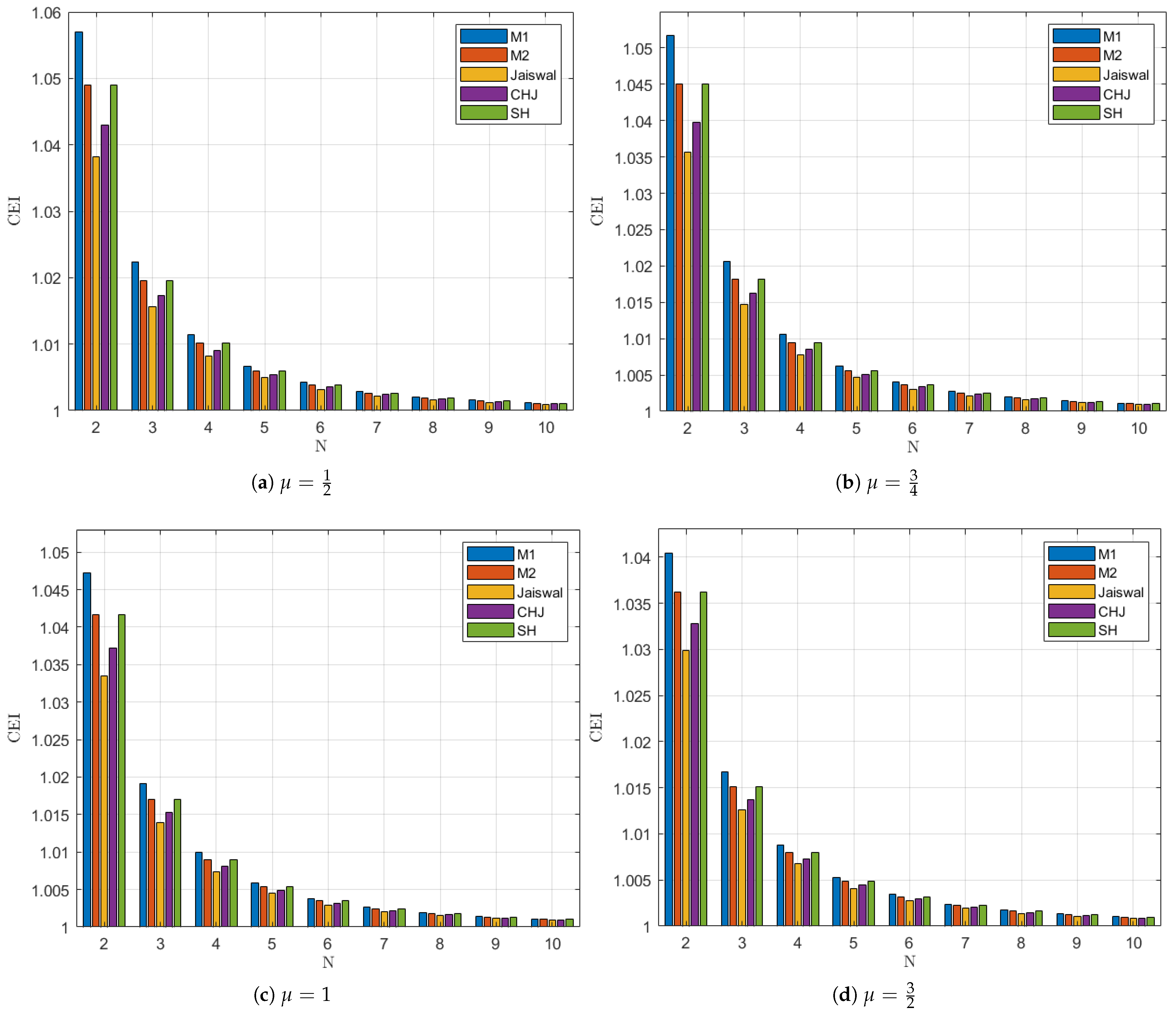
With the results obtained from Table 1, we represent in Figure 1 the performance of the efficiency index for the examined schemes.

Figure 1 shows that $M1$ for $\alpha =0$ has better behavior than all the other methods analyzed. Furthermore, Sharma and $M1$ for $\alpha ={\displaystyle \frac{9}{8}}$ are second in efficiency. It is also shown that as $\mu$ increases, the Computational Efficiency decreases for all schemes.

In the next section, some examples are worked out in order to perform numerical tests.

4. Numerical Results

In this section, several numerical examples are provided to validate the efficiency of our analysis for local convergence (Examples 1–3).

Example 1. 

The van der Waals equation of state (for a vapor) is (see [19,20]):

$$\left(P+{\displaystyle \frac{a}{V^2}}\right)\left(V-b\right)=RT,$$

This equation can be rearranged to the form:

$$P{V}^3-\left(Pb+RT\right)V^2+aV-ab=0$$

in V, where every constant possesses physical significance, with values that can be found in [19]. Let $X=\mathbb{R}$ and $D=\left[0,100\right]$. Choose $P=10,000$ kPa and $T=800$ K. Then, the solution V from the resulting equation is $36.9167$. Applying the conditions given in Theorems 1 and 2, we obtain $L_0=0.1151$, $L=0.1215$ and $M=1.12$. The radii are:

$$\begin{array}{cc}\hfill & \left(C_1\right)-\left(C_3\right):\alpha =0.10,r=0.1575<r_1=3.0365\hfill \\ \hfill & \left(C_4\right):\alpha =0,\overline{r}=0.6397<\overline{r_1}=3.5000\hfill \end{array}$$

The uniqueness radius is:

$$R<{\displaystyle \frac{2}{L_0}}={\displaystyle \frac{2}{0.1151}}=17.38$$

Example 2 

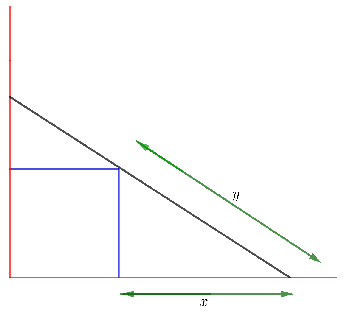
(Beam Design Problem). Here, we examine a beam positioning problem (see [21]), where a beam of length l units is positioned against the edge of a cubical box with one end placed on the floor and the other end positioned against the wall. The box, with sides of 1 units each, is positioned on the floor braced against the wall and one end rests on the floor, as shown in Figure 2.

The triangles formed by the floor, box and beam (lower) and by the box, wall, and beam (upper) are similar.

In this case, the measurement from the base of the wall to where the beam touches the floor is $l=4$. Suppose y represents the length measured from the floor to the edge of the box along the length of the beam, and let x be the distance measured from the bottom of the box to the lower edge of the beam. Let $X=\mathbb{R}$ and $D=\left]0,3\right[$. Then, we have:

$$x^4+2x^3-14x^2+2x+1=0.$$

One positive solution of the equation is the zero $x=2.7609$, and the first derivative is $4x^3+6x^2-28x+2=0$. Applying the conditions given in Theorems 1 and 2, we obtain $L_0=1.87$, $L=1.9723$ and $M=1.1634$. The radii are:

$$\begin{array}{cc}\hfill & \left(C_1\right)-\left(C_3\right):\alpha =0,r=0.0100<r_1=0.1916\hfill \\ \hfill & \left(C_4\right):\alpha =0,\overline{r}=0.0208<\overline{r_1}=0.2143\hfill \end{array}$$

The uniqueness radius is:

$$R<{\displaystyle \frac{2}{L_0}}={\displaystyle \frac{2}{1.87}}=1.0695$$

In Examples 3 and 4, we choose two members of the described iterative method and perform numerical tests to compare them with iterative schemes [13,14,15].

Numerical calculations were executed on a computer with 16 MB RAM and Intel Core i7 processor using MATLAB R2024a software, using variable precision arithmetics with 2000 digits of mantissa. Since we are comparing schemes of high order of convergence, the error tolerance is set at $ϵ={10}^{-100}$, to reduce the risk of significant error accumulation, and therefore, ensure more accurate results.

For each method, the error estimate between two consecutive iterations is $\parallel x_{k+1}-x_k\parallel$ and the residual error is $\parallel \mathcal{T}\left(x_{k+1}\right)\parallel$. The stopping criterium is set at $\parallel x_{k+1}-x_k\parallel +\parallel \mathcal{T}\left(x_{k+1}\right)\parallel <ϵ$. The necessary number of iterations (iter) to converge to the solution is provided.

To validate the theoretical order of convergence p, the ACOC is computed. The execution time, denoted as e-time, required to achieve convergence is displayed (in seconds), based on the average of 10 successive runs for each scheme.

Example 3. 

Let us examine a system of differential equations that describe the motion of an object given by (see [22]):

$${\mathcal{T}}_1^{\prime }\left(x\right)=e^x,F_2^{\prime }\left(y\right)=\left(e-1\right)y+1,F_3^{\prime }\left(z\right)=1$$

with initial conditions ${\mathcal{T}}_1\left(0\right)={\mathcal{T}}_2\left(0\right)={\mathcal{T}}_3\left(0\right)=0$. Let us assume $\mathcal{T}=({\mathcal{T}}_1,{\mathcal{T}}_2,{\mathcal{T}}_3)$. Let $X=Y=R^3,D=\tilde{U}(0,1)$ and $x^{*}={(0,0,0)}^T$. Define function $\mathcal{T}$ on D for $w={(x,y,z)}^T$ by:

$$\mathcal{T}\left(w\right)={\left(e^x-1,{\displaystyle \frac{e-1}{2}}{y}^2+y,z\right)}^T.$$

The Fréchet derivative is given by:

$${\mathcal{T}}^{\prime }\left(\nu \right)=\left[\begin{array}{ccc}{e}^x& 0& 0\\ 0& (e-1)y+1& 0\\ 0& 0& 1\end{array}\right]$$

Applying the conditions given in Theorems 1 and 2, we obtain $L_0=e-1$ and $L=M=e^{{\displaystyle \frac{1}{e-1}}}$. The radii are:

$$\begin{array}{cc}\hfill & \left(C_1\right)-\left(C_3\right):\alpha =0.10,r=0.0127<r_1=0.2607\hfill \\ \hfill & \left(C_4\right):\alpha =0,\overline{r}=0.3449<\overline{r_1}=0.4147\hfill \end{array}$$

The uniqueness radius is:

$$R<{\displaystyle \frac{2}{L_0}}={\displaystyle \frac{2}{e-1}}=1.1640$$

The results from

Table 2. Numerical performance of iterative schemes for a nonlinear system of equations.

Method	$\tilde{\mathit{x}}$	$∥{\mathit{x}}_{\mathit{k}+1}-{\mathit{x}}_{\mathit{k}}∥$	$∥\mathcal{T}\left({\mathit{x}}_{\mathit{k}+1}\right)∥$	Iter	ACOC	e-Time
$x_0={\left[0.50.50.5\right]}^T$
$M{1}_{(\alpha =0)}$	${\left[1.18\times {10}^{-40},0,0\right]}^T$	$1.17\times {10}^{-31}$	$1.17\times {10}^{-31}$	4	3.9754	0.33349
$M{1}_{(\alpha ={\displaystyle \frac{9}{8}})}$	nc	$1.13\times {10}^{17}$	$9.22\times {10}^{51}$	50	1.00000	3.68628
Jaiswal	${\left[4.43\times {10}^{-41},-7.24\times {10}^{-71},0\right]}^T$	$8.49\times {10}^{-32}$	$8.49\times {10}^{-32}$	4	3.9972	0.32919
CHJ	${\left[2.7\times {10}^{-43},-1.19\times {10}^{-66},0\right]}^T$	$1.62\times {10}^{-27}$	$1.62\times {10}^{-27}$	4	3.9454	0.35557
Sharma	nc	$1.13\times {10}^{17}$	$9.22\times {10}^{51}$	50	1.00000	3.60789

show that scheme $M1$ for $\alpha =0$ converges adequately to the solution, and so do CHJ and Jaiswal methods. Scheme $M1$ for $\alpha ={\displaystyle \frac{9}{8}}$ does not converge to the solution. We must remember that, according to Theorem 1, the values of $\alpha$ for we can guarantee convergence are those in $\left]-{\displaystyle \frac{3}{8}},{\displaystyle \frac{1}{8}}\right[$. The Sharma scheme does not converge to the solution either.

Example 4. 

Consider the system of equations of size $n=20$, with the expression:

$$x_i-cos\left(2x_i-x_1-x_2-x_3-x_4\right)=0;i=1,2,\dots ,n$$

with $x^{*}={(0.5149,0.5149,\dots ,0.5149)}^T$.

In a similar way to Example 3, the results from

Table 3. Numerical performance of iterative schemes for a nonlinear system of equations.

Method	$\tilde{\mathit{x}}$	$∥{\mathit{x}}_{\mathit{k}+1}-{\mathit{x}}_{\mathit{k}}∥$	$∥\mathcal{T}\left({\mathit{x}}_{\mathit{k}+1}\right)∥$	Iter	ACOC	e-Time
$x_0={\left[1,1,\dots ,1\right]}^T$
$M{1}_{(\alpha =0)}$	${\left[0.514933,0.514933,\dots ,0.514933\right]}^T$	$1.18\times {10}^{-11}$	$3.21\times {10}^{-11}$	3	3.6538	1.78310
$M{1}_{(\alpha ={\displaystyle \frac{9}{8}})}$	nc	$3.36\times {10}^{30}$	$1.03\times {10}^{31}$	50	-	33.70610
Jaiswal	${\left[0.514933,0.514933,\dots ,0.514933\right]}^T$	$1.23\times {10}^{-11}$	$3.35\times {10}^{-11}$	3	3.6476	1.80741
CHJ	${\left[0.514933,0.514933,\dots ,0.514933\right]}^T$	$1.73\times {10}^{-11}$	$4.69\times {10}^{-11}$	3	3.5972	1.78408
Sharma	nc	$3.36\times {10}^{30}$	$1.03\times {10}^{31}$	50	-	40.46302

show that schemes $M1$ for $\alpha =0$, CHJ and Jaiswal converge to the solution. Schemes $M1$ for $\alpha ={\displaystyle \frac{9}{8}}$ and Sharma fail to converge. According to Theorem 1, the values of $\alpha$ for we can guarantee convergence are those in $\left]-{\displaystyle \frac{3}{8}},{\displaystyle \frac{1}{8}}\right[$.

5. Conclusions

The current paper presents a local convergence study of a class family of iterative schemes within Banach spaces, provided that the Fréchet derivative satisfies the Lipschitz continuity condition. For the convergence balls, the radii have been obtained, according to the existence and uniqueness Theorem. In the examples shown, scheme (1) gives smaller radii without using M.

All schemes have the same Ostrowski’s Efficiency Index, since this index focuses exclusively on the number of functional evaluations and the order of convergence. Scheme (1) has better behavior for $\alpha =0$ (in terms of Computational Efficiency) than all the other methods analyzed. Furthermore, Sharma and $M1$ for $\alpha ={\displaystyle \frac{9}{8}}$ are second in efficiency.

For the Computational Efficiency Index was introduced a correction factor $\mu$, which transformed the number of evaluations into a number of operations. The value of this parameter can be tested computationally to establish a relationship between evaluating a function and performing arithmetic operations. Nevertheless, the key is to use the same value as in other studies to ensure a proper comparison.

Future works related to this line of research and based on these results are focused on semilocal convergence analysis using majorizing sequences. This study extends the scope of local convergence by not only establishing conditions under which an initial approximation leads to a solution, but also providing the domain of existence of that solution, thus being valid for proving the existence of a solution to a problem for which prior information was not known. This analysis is particularly valuable for demonstrating the existence of solutions and ensuring the reliability of iterative algorithms in functional analysis, optimization, and numerical applications.