
Activation-Based Pruning of Neural Networks


Abstract
1. Introduction
2. Related Work
2.1. Low-Rank Matrix Approximation
2.2. Structured/Unstructured Pruning
2.3. Importance-Based Pruning
2.4. Iterative/One-Shot Pruning
2.5. When to Prune
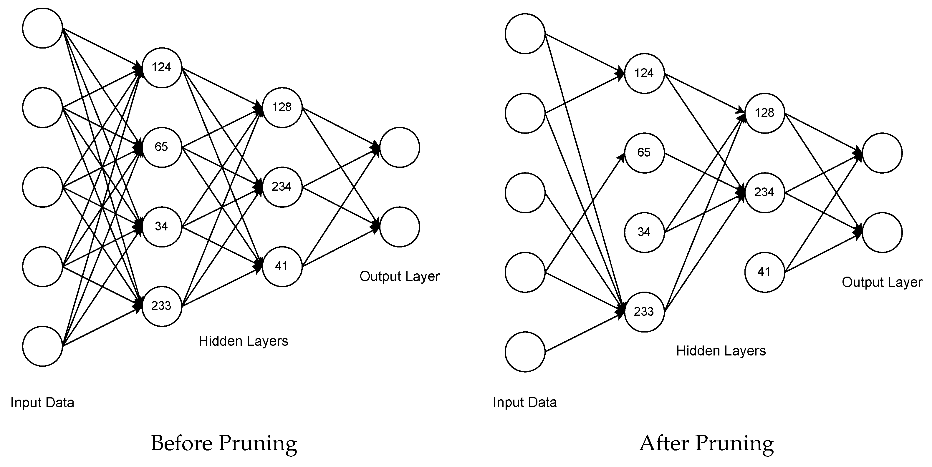
3. Methodology
3.1. Global Activation-Based Pruning
| Algorithm 1 Global activation-based pruning. |
|
| Algorithm 2 Update neuron. |
|
| Algorithm 3 Prune. |
|
3.2. Local Activation-Based Pruning
| Algorithm 4 Local activation-based pruning. |
|
| Algorithm 5 Update neuron. |
|
| Algorithm 6 Prune. |
|
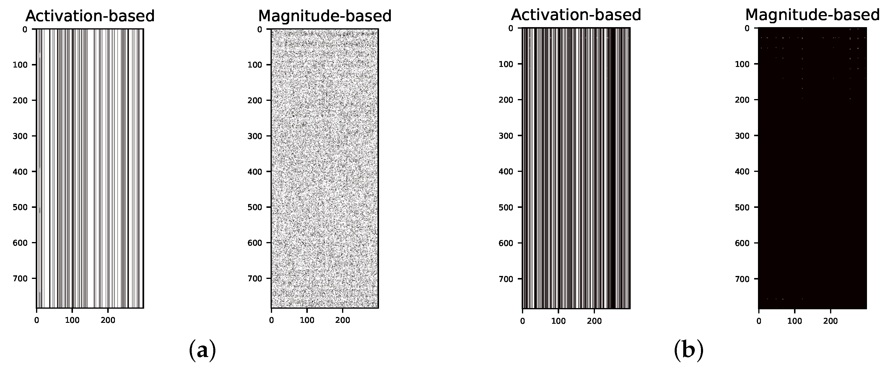
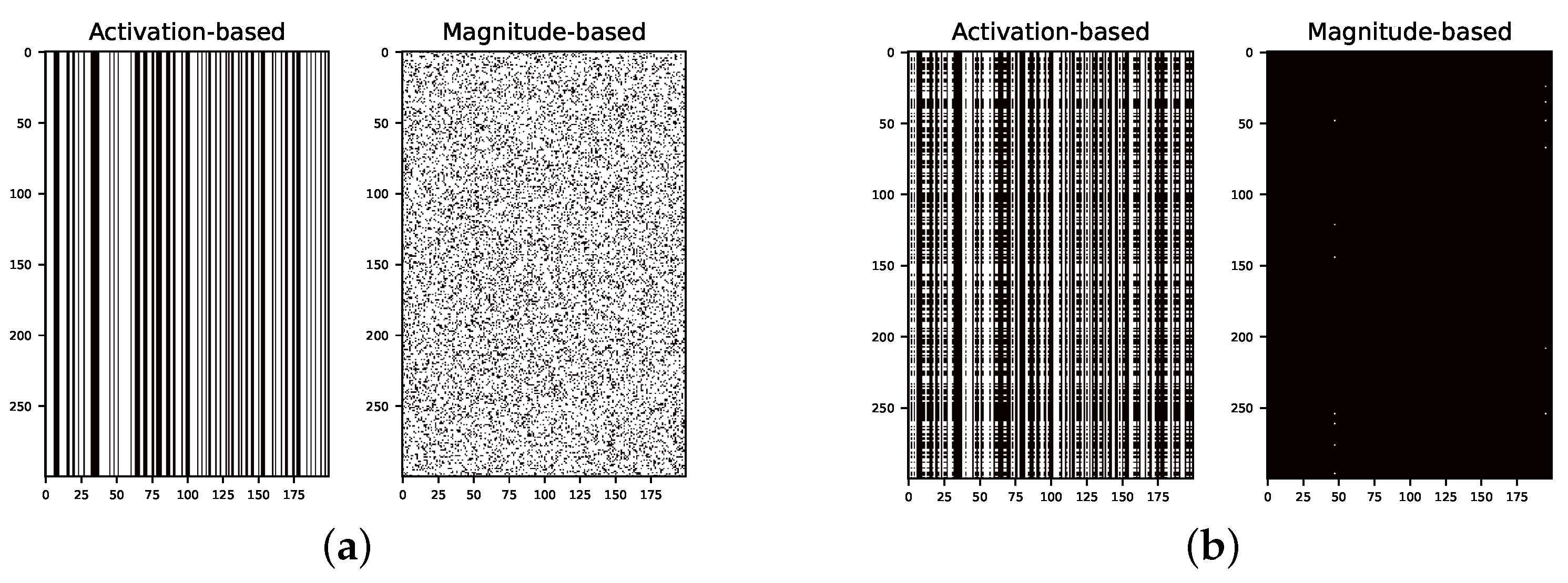
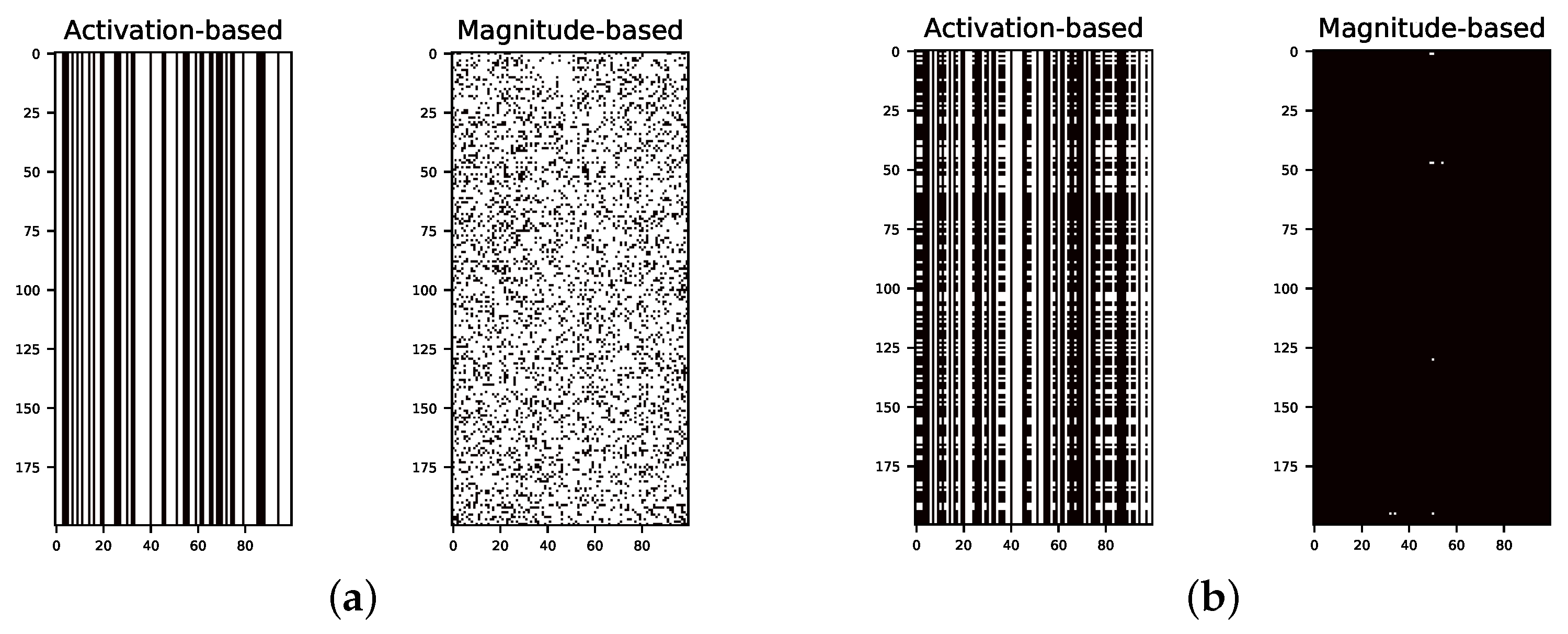
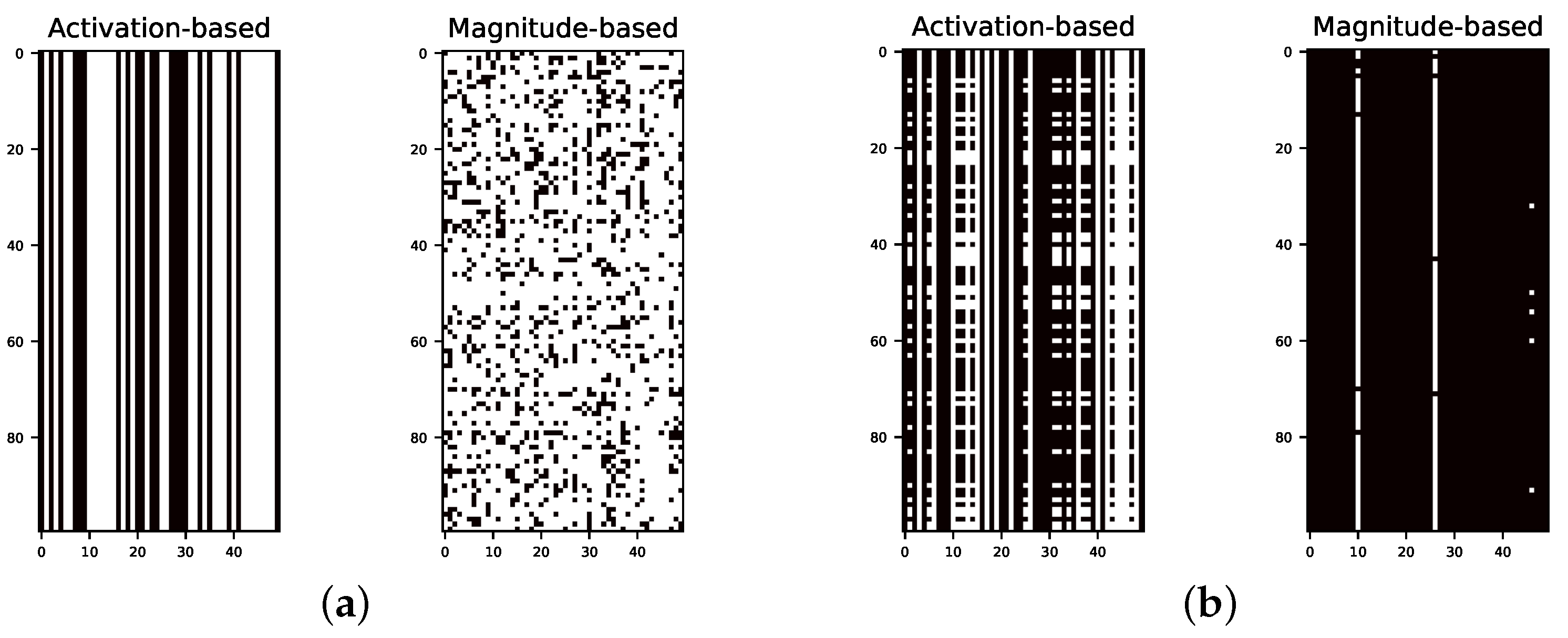
3.3. Activation- vs. Magnitude-Based Pruning
3.4. Principal Component Analysis of Hidden Layers
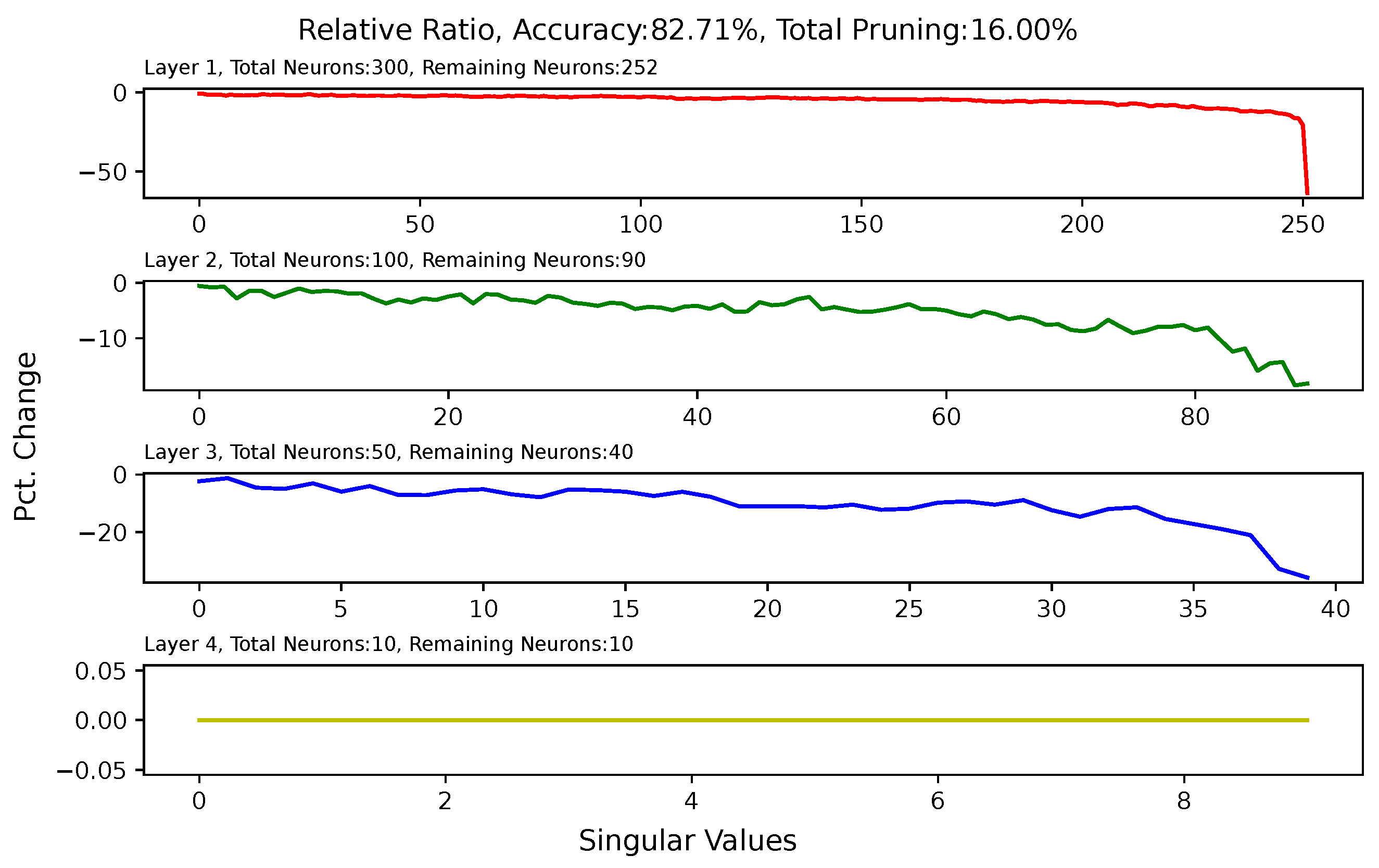
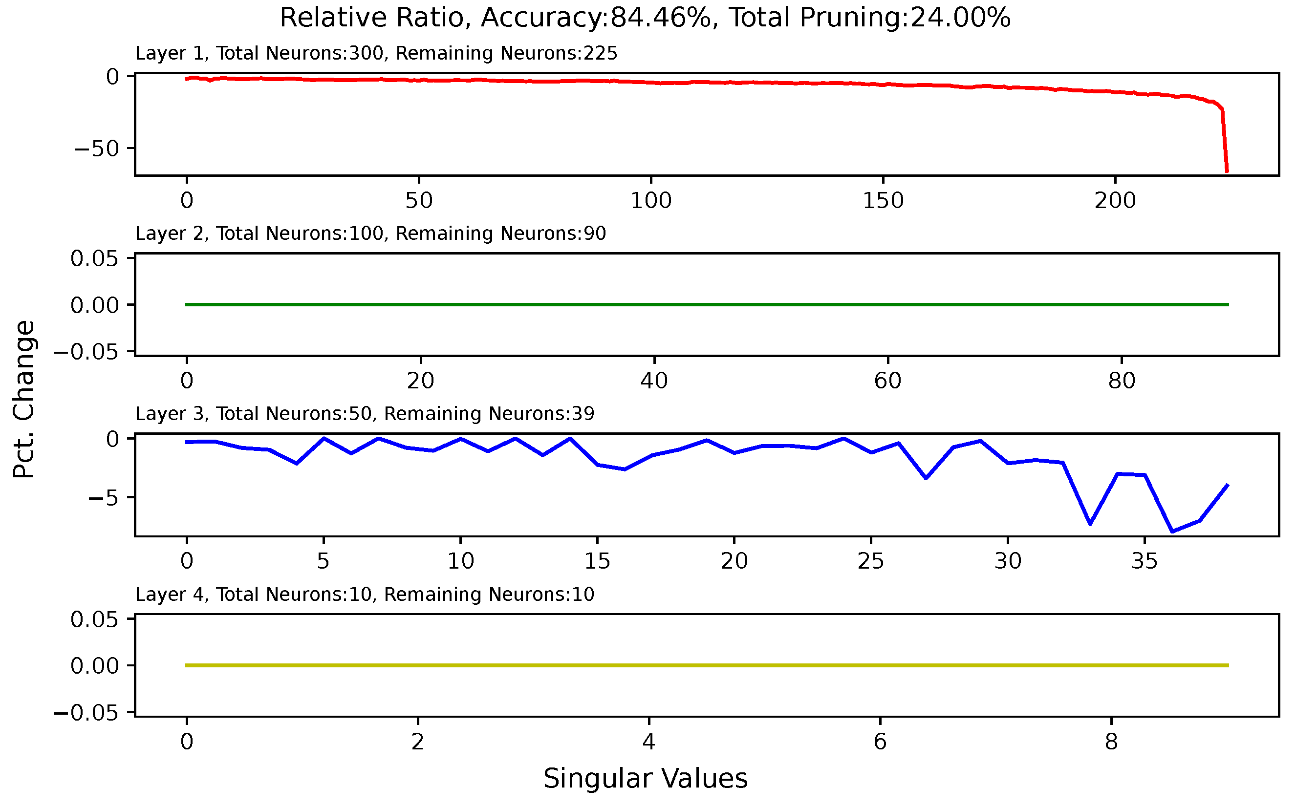
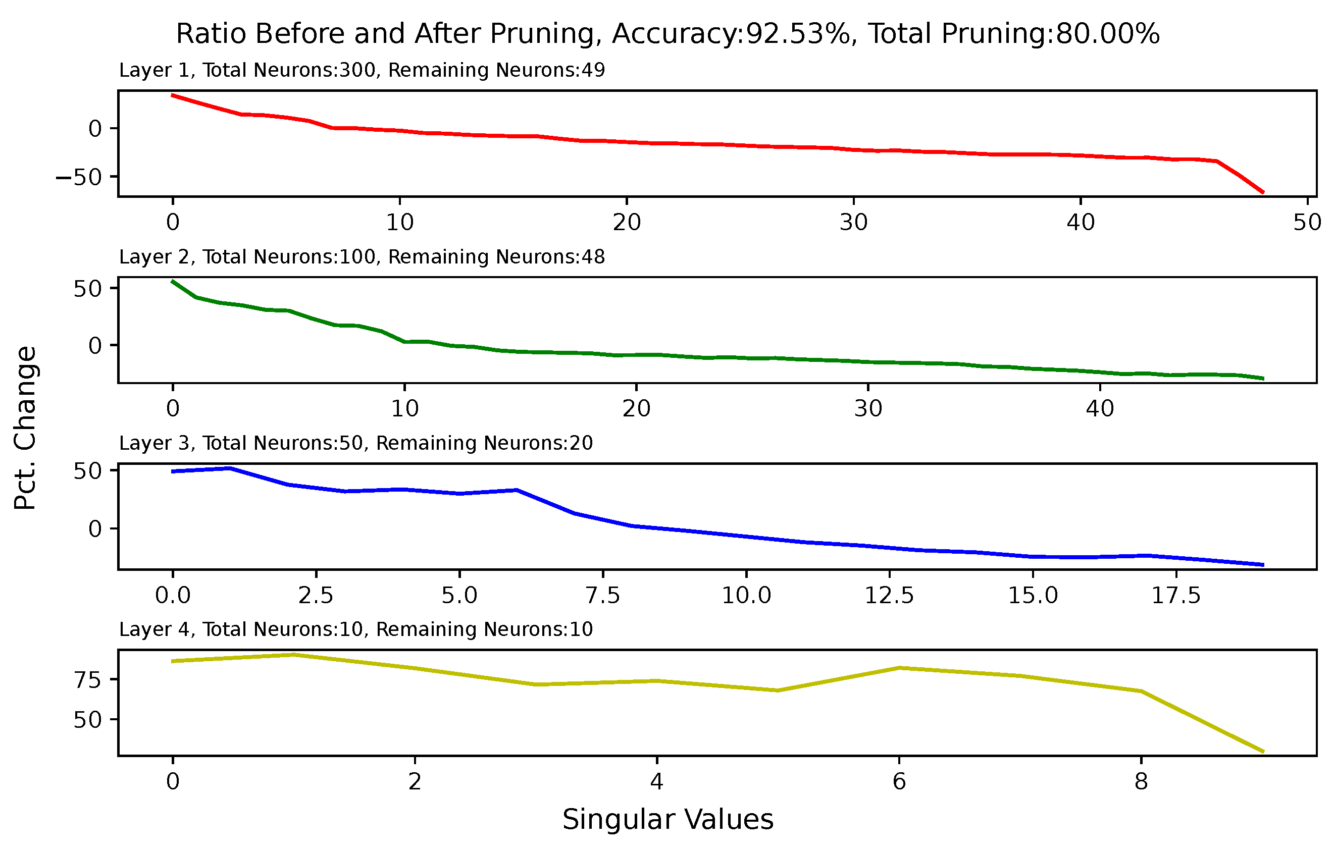
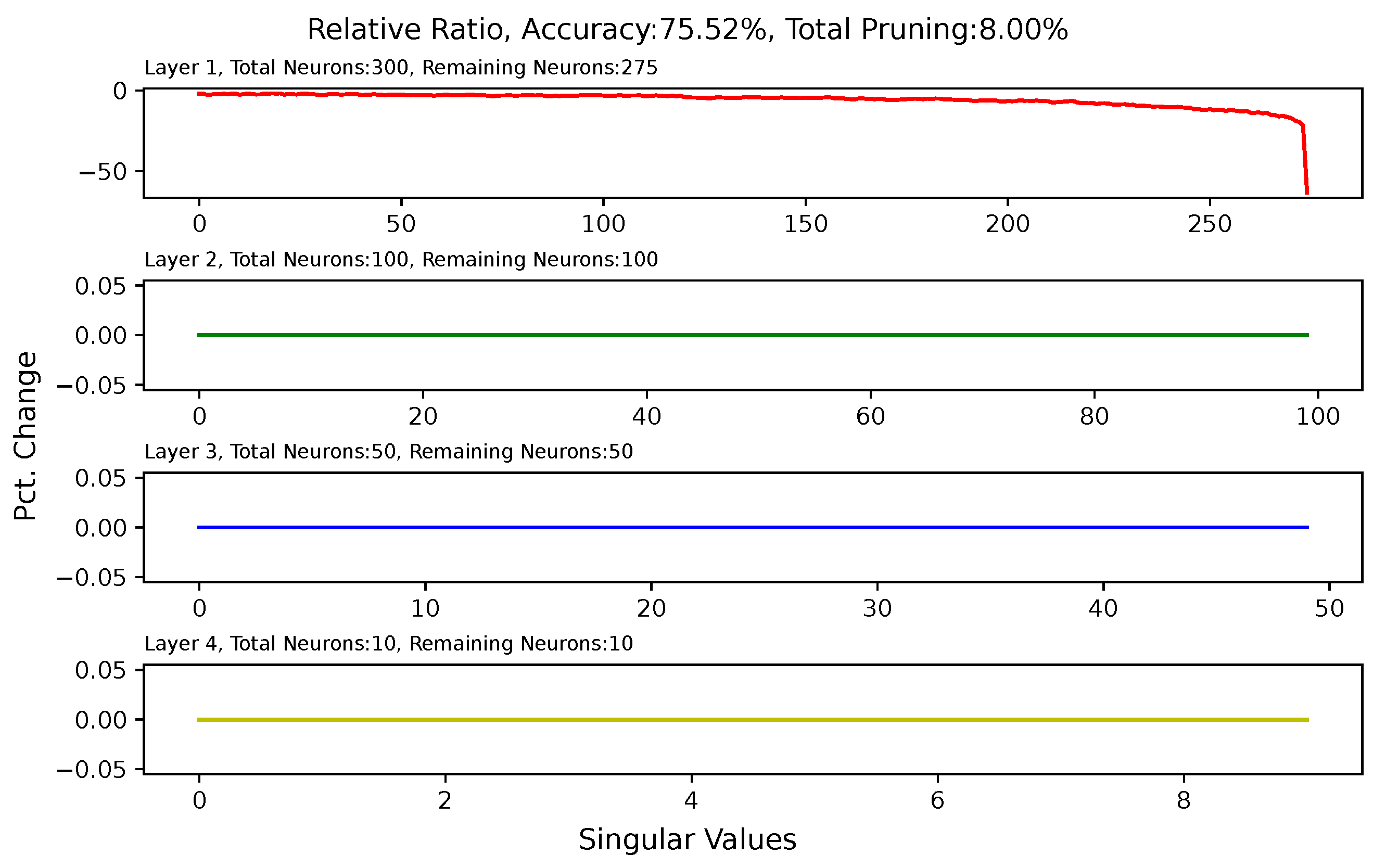
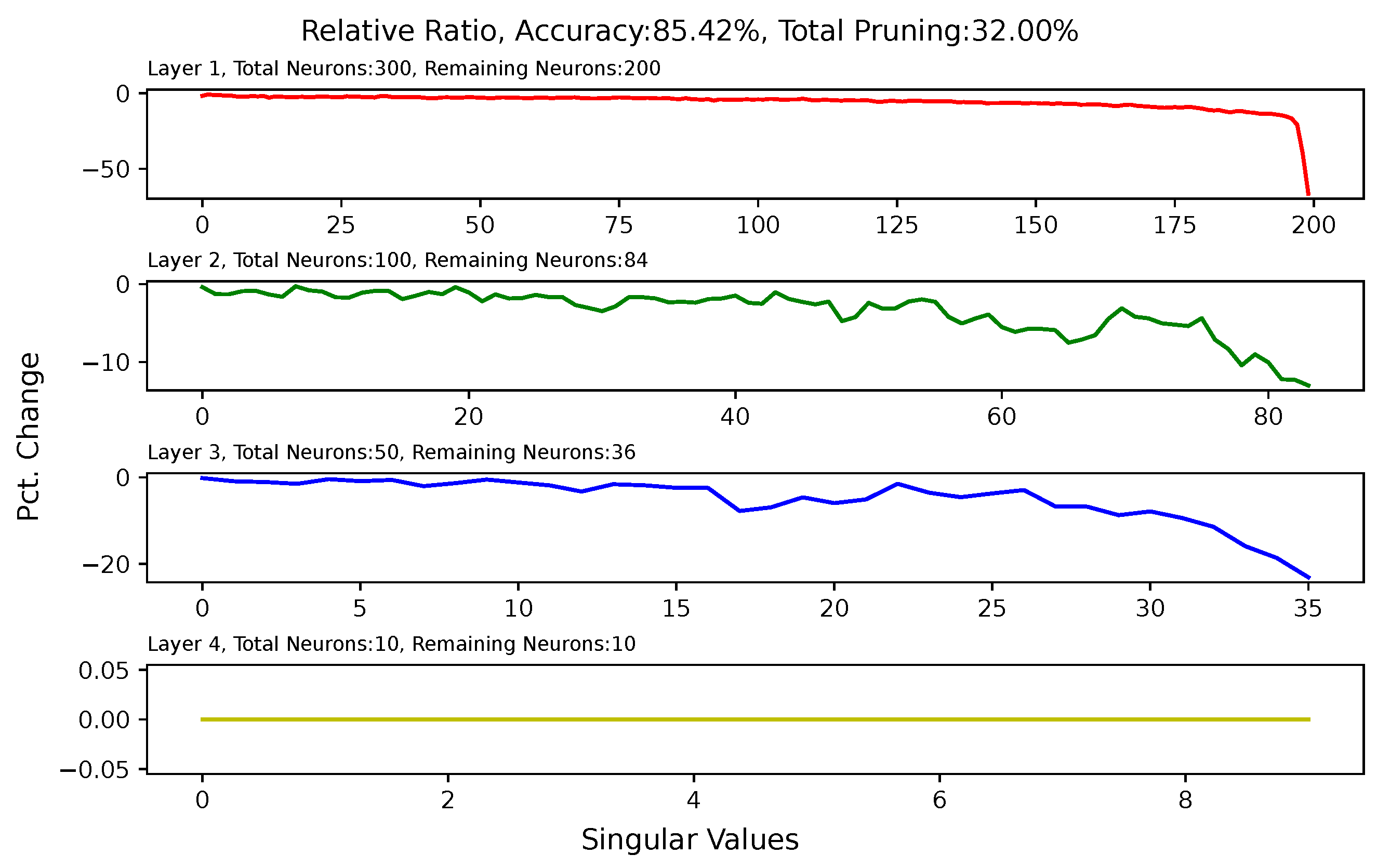
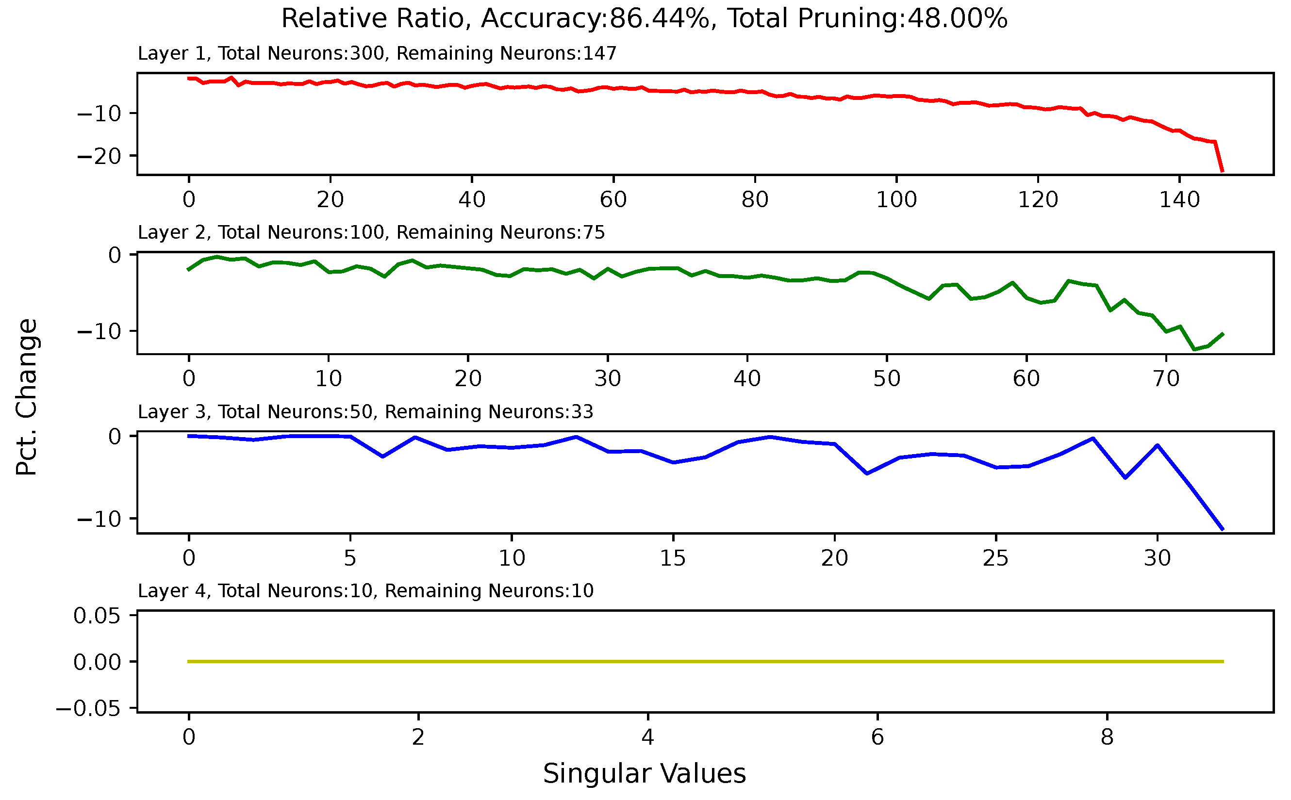
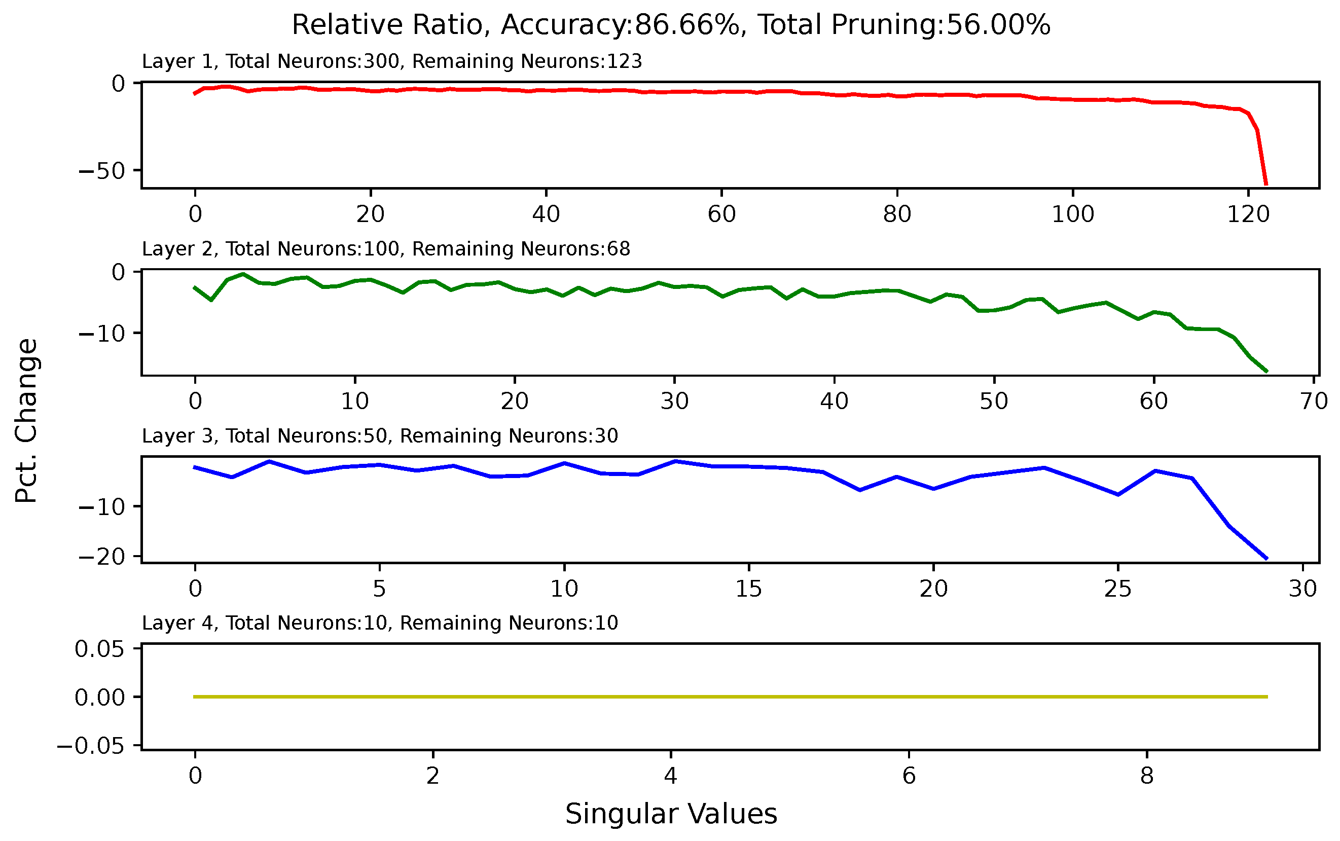
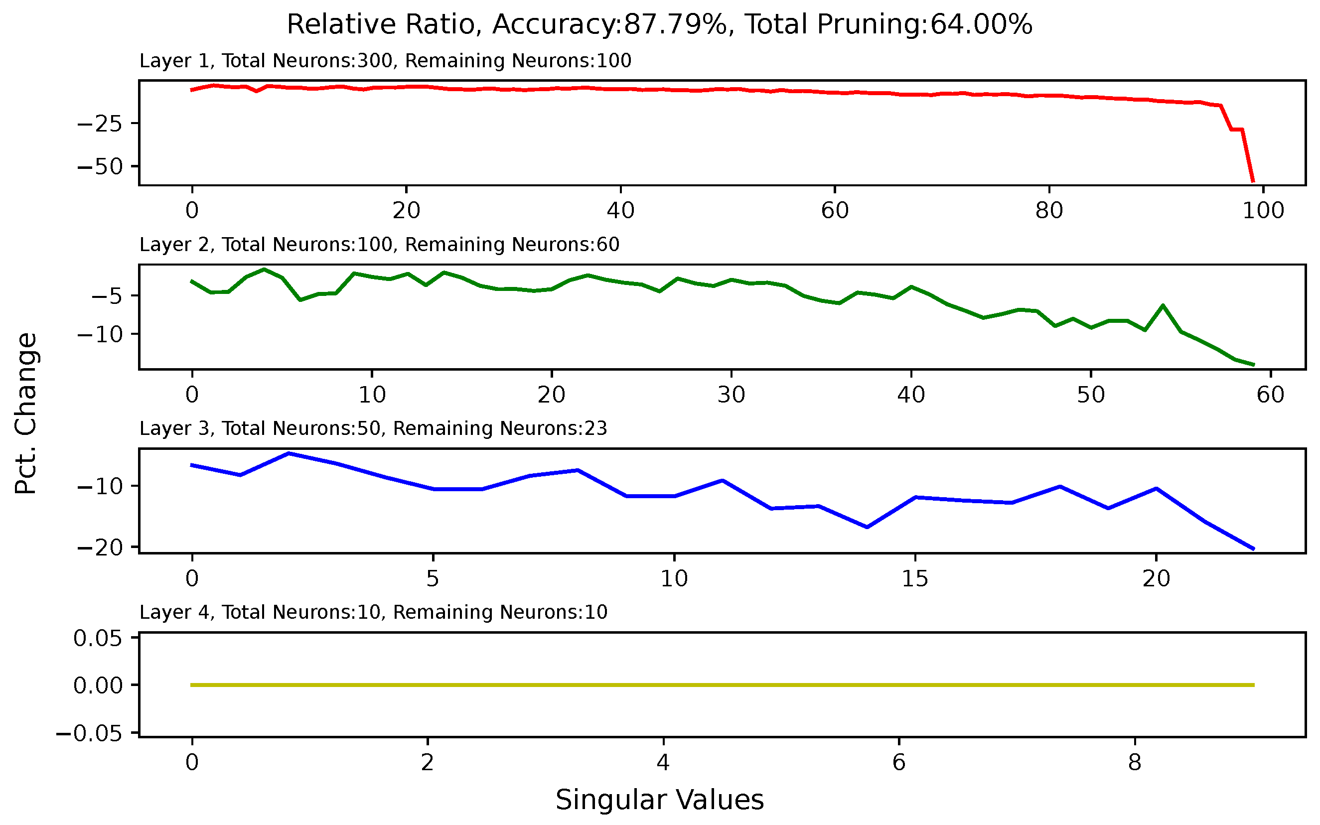
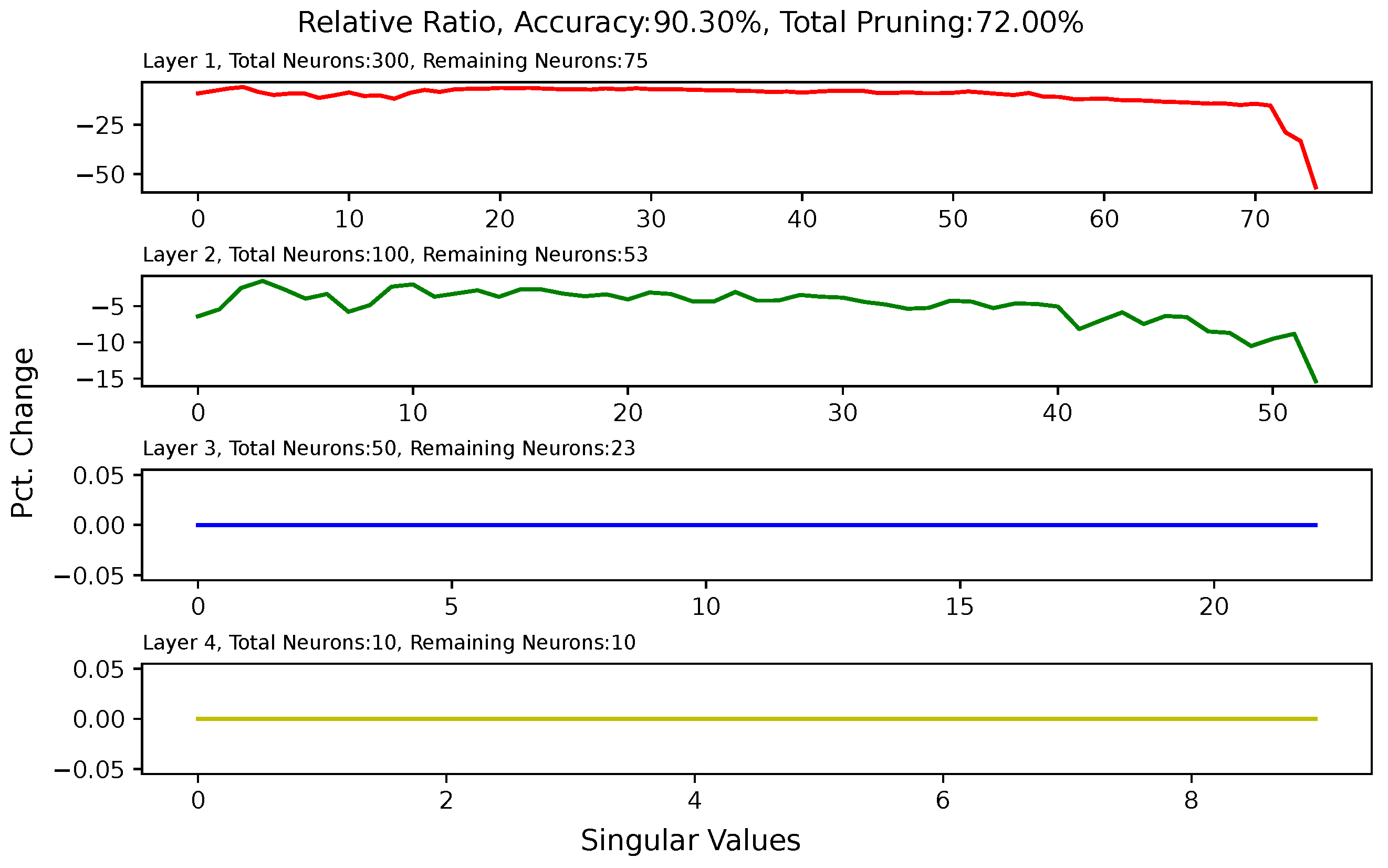
3.5. Effect of Pruning on Singular Values of Matrices of Hidden Layers
4. Experiment Settings
4.1. Common Setting
4.2. Global Activation-Based Pruning Setting
4.3. Local Activation-Based Pruning Setting
5. Results and Discussion
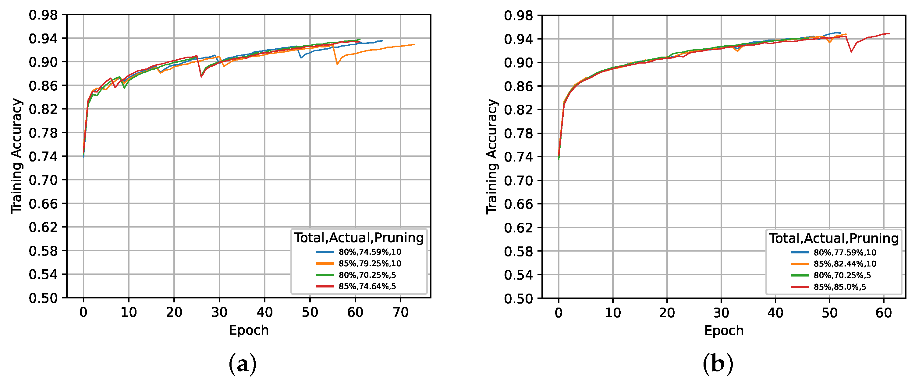
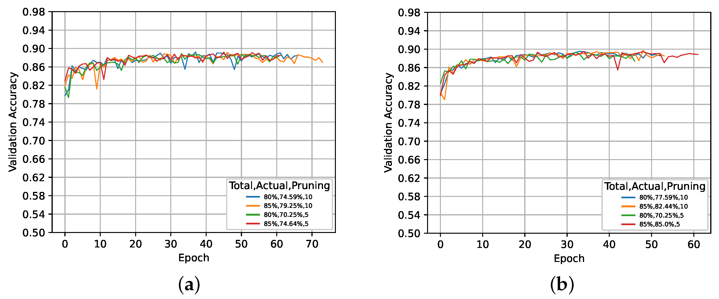
5.1. Global Activation-Based Pruning
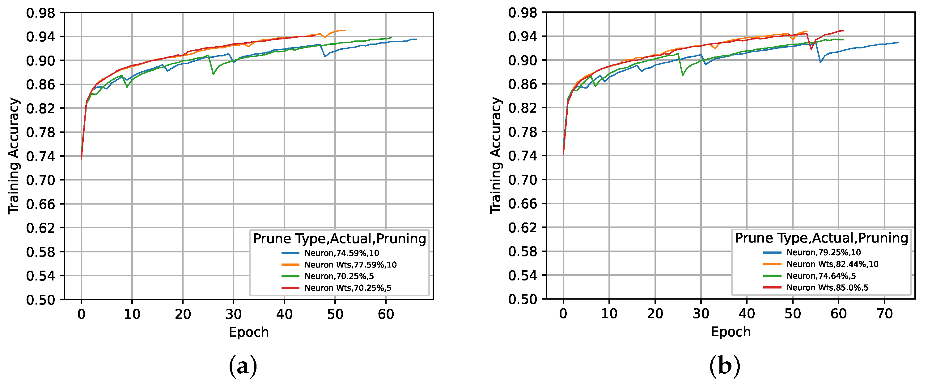
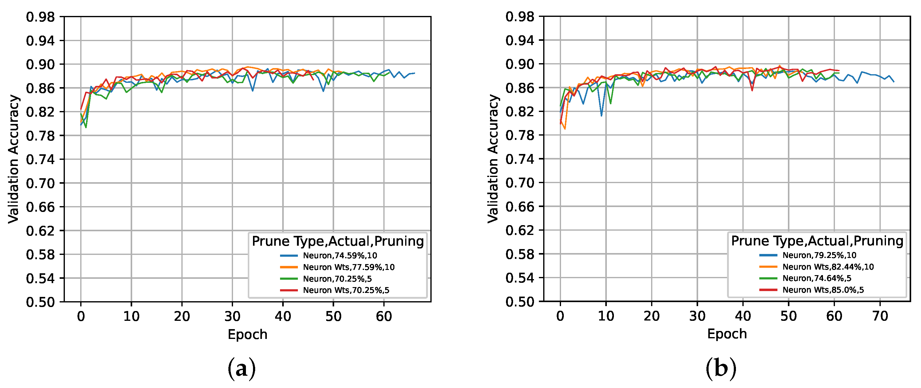
5.2. Local Activation-Based Pruning
5.3. Activation- vs. Magnitude-Based Pruning
5.4. Comparative Analysis
5.4.1. Activation-Based Pruning Methods
5.4.2. Activation-Based Pruning against Similar Models
5.5. Principal Component Analysis of Hidden Layers
5.6. Analysis of Singular Value Changes in Each Layer
6. Conclusions
Author Contributions
Funding
Data Availability Statement
Conflicts of Interest
Abbreviations
| SVD | singular-value decomposition |
| WNNM | weighted nuclear norm minimization |
| NNM | nuclear norm minimization |
| ReLU | Rectified Linear Unit |
| SGD | Stochastic Gradient Descent |
| PCA | principal component analysis |
Appendix A. Singular-Value Minimization


Appendix B. Heat Map for Pruned and Retrained Network


References
- Molchanov, P.; Tyree, S.; Karras, T.; Aila, T.; Kautz, J. Pruning Convolutional Neural Networks for Resource Efficient Inference. arXiv 2017, arXiv:1611.06440. [Google Scholar]
- Han, S.; Pool, J.; Tran, J.; Dally, W. Learning both Weights and Connections for Efficient Neural Network. In Advances in Neural Information Processing Systems; Cortes, C., Lawrence, N., Lee, D., Sugiyama, M., Garnett, R., Eds.; Curran Associates, Inc.: Red Hook, NY, USA, 2015; Volume 28. [Google Scholar]
- Hu, H.; Peng, R.; Tai, Y.W.; Tang, C.K. Network Trimming: A Data-Driven Neuron Pruning Approach towards Efficient Deep Architectures. arXiv 2016, arXiv:1607.03250. [Google Scholar]
- Li, H.; Kadav, A.; Durdanovic, I.; Samet, H.; Graf, H.P. Pruning Filters for Efficient ConvNets. arXiv 2017, arXiv:1608.08710. [Google Scholar]
- Frankle, J.; Carbin, M. The Lottery Ticket Hypothesis: Finding Sparse, Trainable Neural Networks. In Proceedings of the International Conference on Learning Representations, New Orleans, LA, USA, 6–9 May 2019. [Google Scholar]
- Guo, Y.; Yao, A.; Chen, Y. Dynamic Network Surgery for Efficient DNNs. In Advances in Neural Information Processing Systems; Lee, D., Sugiyama, M., Luxburg, U., Guyon, I., Garnett, R., Eds.; Curran Associates, Inc.: Red Hook, NY, USA, 2016; Volume 29. [Google Scholar]
- Han, S.; Mao, H.; Dally, W.J. Deep Compression: Compressing Deep Neural Networks with Pruning, Trained Quantization and Huffman Coding. arXiv 2016, arXiv:1510.00149. [Google Scholar]
- Zhu, M.; Gupta, S. To prune, or not to prune: Exploring the efficacy of pruning for model compression. arXiv 2017, arXiv:1710.01878. [Google Scholar]
- Shlens, J. A Tutorial on Principal Component Analysis. arXiv 2014, arXiv:1404.1100. [Google Scholar]
- Swaminathan, S.; Garg, D.; Kannan, R.; Andres, F. Sparse low rank factorization for deep neural network compression. Neurocomputing 2020, 398, 185–196. [Google Scholar] [CrossRef]
- Yang, H.; Tang, M.; Wen, W.; Yan, F.; Hu, D.; Li, A.; Li, H.; Chen, Y. Learning Low-Rank Deep Neural Networks via Singular Vector Orthogonality Regularization and Singular Value Sparsification. In Proceedings of the IEEE/CVF Conference on Computer Vision and Pattern Recognition (CVPR) Workshops, Virtually, 14–19 June 2020. [Google Scholar]
- He, Y.; Zhang, X.; Sun, J. Channel Pruning for Accelerating Very Deep Neural Networks. In Proceedings of the 2017 IEEE International Conference on Computer Vision (ICCV), Venice, Italy, 22–29 October 2017; pp. 1398–1406. [Google Scholar] [CrossRef]
- Gray, S.; Radford, A.; Kingma, D.P. GPU Kernels for Block-Sparse Weights. arXiv 2017, arXiv:1711.09224. [Google Scholar]
- Kalchbrenner, N.; Elsen, E.; Simonyan, K.; Noury, S.; Casagrande, N.; Lockhart, E.; Stimberg, F.; van den Oord, A.; Dieleman, S.; Kavukcuoglu, K. Efficient Neural Audio Synthesis. In Proceedings of the 35th International Conference on Machine Learning, Stockholm, Sweden, 10–15 July 2018; Dy, J., Krause, A., Eds.; Proceedings of Machine Learning Research. Volume 80, pp. 2410–2419. [Google Scholar]
- Frankle, J.; Dziugaite, G.K.; Roy, D.M.; Carbin, M. Stabilizing the Lottery Ticket Hypothesis. arXiv 2020, arXiv:1903.01611. [Google Scholar]
- Yu, R.; Li, A.; Chen, C.F.; Lai, J.H.; Morariu, V.I.; Han, X.; Gao, M.; Lin, C.Y.; Davis, L.S. NISP: Pruning Networks Using Neuron Importance Score Propagation. In Proceedings of the 2018 IEEE/CVF Conference on Computer Vision and Pattern Recognition, Salt Lake City, UT, USA, 18–23 June 2018; pp. 9194–9203. [Google Scholar] [CrossRef]
- Molchanov, D.; Ashukha, A.; Vetrov, D. Variational Dropout Sparsifies Deep Neural Networks. In Proceedings of the 34th International Conference on Machine Learning, Sydney, NSW, Australia, 6–11 August 2017; Precup, D., Teh, Y.W., Eds.; Proceedings of Machine Learning Research. Volume 70, pp. 2498–2507. [Google Scholar]
- Mariet, Z.; Sra, S. Diversity Networks: Neural Network Compression Using Determinantal Point Processes. arXiv 2017, arXiv:1511.05077. [Google Scholar]
- Lee, N.; Ajanthan, T.; Torr, P. SNIP: Single-Shot Network Pruning Based on Connection Sensitivity. In Proceedings of the International Conference on Learning Representations, New Orleans, LA, USA, 6–9 May 2019. [Google Scholar]
- Liu, Z.; Sun, M.; Zhou, T.; Huang, G.; Darrell, T. Rethinking the Value of Network Pruning. In Proceedings of the International Conference on Learning Representations, New Orleans, LA, USA, 6–9 May 2019. [Google Scholar]
- Yuan, X.; Savarese, P.; Maire, M. Growing Efficient Deep Networks by Structured Continuous Sparsification. arXiv 2020, arXiv:2007.15353. [Google Scholar]
- Wang, C.; Zhang, G.; Grosse, R. Picking Winning Tickets Before Training by Preserving Gradient Flow. arXiv 2020, arXiv:2002.07376. [Google Scholar]
- Tanaka, H.; Kunin, D.; Yamins, D.L.; Ganguli, S. Pruning neural networks without any data by iteratively conserving synaptic flow. In Advances in Neural Information Processing Systems; Larochelle, H., Ranzato, M., Hadsell, R., Balcan, M., Lin, H., Eds.; Curran Associates, Inc.: Red Hook, NY, USA, 2020; Volume 33, pp. 6377–6389. [Google Scholar]
- Frantar, E.; Alistarh, D. SparseGPT: Massive Language Models Can Be Accurately Pruned in One-Shot. arXiv 2023, arXiv:2301.00774. [Google Scholar]
- Sun, M.; Liu, Z.; Bair, A.; Kolter, J.Z. A Simple and Effective Pruning Approach for Large Language Models. arXiv 2023, arXiv:2306.11695. [Google Scholar]
- Gu, S.; Zhang, L.; Zuo, W.; Feng, X. Weighted Nuclear Norm Minimization with Application to Image Denoising. In Proceedings of the 2014 IEEE Conference on Computer Vision and Pattern Recognition, Columbus, OH, USA, 23–28 June 2014; pp. 2862–2869. [Google Scholar] [CrossRef]
- Zha, Z.; Wen, B.; Zhang, J.; Zhou, J.; Zhu, C. A Comparative Study for the Nuclear Norms Minimization Methods. In Proceedings of the 2019 IEEE International Conference on Image Processing (ICIP), Taipei, Taiwan, 22–25 September 2019; pp. 2050–2054. [Google Scholar] [CrossRef]


| Pruning Type | Time | Space |
|---|---|---|
| Global | ||
| Local |
| No. | Pruning Iterations | Pruning Type | Epochs | Target Prune % | Pruning Achieved | Top 1% Accuracy | Top 5% Accuracy | ||||
|---|---|---|---|---|---|---|---|---|---|---|---|
| Training | Validation | Test | Training | Validation | Test | ||||||
| S1 | NA | Standard | 46 | NA | NA | 10.19 | 8.17 | 8.22 | 69.10 | 68.72 | 69.40 |
| G1 | 5 | Neurons | 62 | 80 | 70.25 | 10.24 | 9.75 | 10.16 | 70.45 | 66.47 | 65.69 |
| G2 | 5 | Neurons | 62 | 85 | 74.64 | 10.13 | 9.23 | 9.54 | 72.23 | 71.47 | 71.67 |
| G3 | 5 | Neurons & Weights | 47 | 80 | 70.25 | 10.13 | 9.35 | 9.66 | 81.30 | 81.50 | 81.83 |
| G4 | 5 | Neurons & Weights | 62 | 85 | 85.00 | 10.15 | 9.00 | 9.46 | 66.59 | 66.65 | 66.77 |
| G5 | 10 | Neurons | 67 | 80 | 74.59 | 10.25 | 9.32 | 9.57 | 80.99 | 80.57 | 80.24 |
| G6 | 10 | Neurons | 74 | 85 | 79.25 | 10.17 | 9.62 | 9.69 | 71.44 | 65.10 | 64.99 |
| G7 | 10 | Neurons & Weights | 53 | 80 | 77.59 | 10.16 | 12.17 | 12.30 | 77.19 | 79.60 | 79.23 |
| G8 | 10 | Neurons & Weights | 54 | 85 | 82.44 | 10.15 | 11.42 | 11.58 | 78.35 | 78.45 | 79.31 |
| No. | Pruning Type | Epochs | Pruning Achieved | Training Accuracy | Validation Accuracy | Test Accuracy | Top 1% Accuracy | Top 5% Accuracy | ||||
|---|---|---|---|---|---|---|---|---|---|---|---|---|
| Training | Validation | Test | Training | Validation | Test | |||||||
| S | Standard | 46 | NA | 95.64 | 85.68 | 84.35 | 10.19 | 8.17 | 8.22 | 69.10 | 68.72 | 69.40 |
| L1 | Neurons | 88 | 79.88 | 93.12 | 88.02 | 87.56 | 10.22 | 11.08 | 10.83 | 64.33 | 63.37 | 64.09 |
| L2 | Neurons | 88 | 84.85 | 92.29 | 86.73 | 86.79 | 10.18 | 12.12 | 11.99 | 72.81 | 73.55 | 74.67 |
| L3 | Neurons & Weights | 75 | 79.88 | 93.29 | 87.92 | 87.11 | 10.19 | 7.73 | 8.01 | 86.36 | 84.92 | 85.29 |
| L4 | Neurons & Weights | 73 | 84.87 | 92.83 | 87.62 | 86.94 | 10.23 | 12.10 | 12.10 | 74.26 | 75.92 | 75.64 |
| Model | Activation Type | Pruning Percentage | Training Accuracy | Validation Accuracy | Test Accuracy |
|---|---|---|---|---|---|
| Magnitude | 80.00 | 91.79 | 92.35 | 88.72 | |
| Activation-based | Neurons | 79.88 | 93.12 | 88.02 | 87.56 |
| Activation-based | Neurons & Weights | 79.88 | 93.29 | 87.92 | 87.11 |
| Pruning Type | ≈kFLOPS | Pct. Reduction |
|---|---|---|
| M | 129 | 79.87 |
| G1 | 191 | 70.25 |
| G2 | 163 | 74.64 |
| G3 | 191 | 70.25 |
| G4 | 96 | 85.00 |
| G5 | 163 | 74.59 |
| G6 | 133 | 79.25 |
| G7 | 144 | 77.59 |
| G8 | 113 | 82.44 |
| L1 | 129 | 79.88 |
| L2 | 97 | 84.85 |
| L3 | 129 | 79.88 |
| L4 | 97 | 84.87 |
| Model | Pruning Type | Epochs | Training Accuracy | Validation Accuracy | Test Accuracy | Top 1% Accuracy | Top 5% Accuracy | ||||
|---|---|---|---|---|---|---|---|---|---|---|---|
| Training | Validation | Test | Training | Validation | Test | ||||||
| M | Magnitude | 9 | 95.01 | 87.37 | 87.01 | 10.23 | 14.10 | 14.09 | 66.62 | 74.13 | 74.85 |
| G1 | Neuron | 21 | 95.24 | 86.55 | 85.99 | 10.10 | 7.57 | 7.82 | 70.90 | 62.45 | 62.52 |
| G2 | Neuron | 24 | 95.34 | 86.97 | 86.08 | 10.10 | 7.58 | 7.73 | 71.26 | 70.43 | 70.68 |
| G3 | Neuron | 24 | 95.29 | 88.73 | 88.50 | 10.18 | 10.17 | 10.51 | 79.96 | 84.55 | 84.22 |
| G4 | Neuron | 23 | 94.69 | 87.78 | 87.41 | 10.13 | 9.28 | 9.93 | 76.62 | 78.15 | 78.40 |
| G5 | Neuron & Weights | 8 | 93.72 | 87.65 | 86.94 | 10.11 | 9.15 | 9.23 | 82.72 | 73.02 | 73.29 |
| G6 | Neuron & Weights | 17 | 95.22 | 86.35 | 85.79 | 10.15 | 7.70 | 8.23 | 67.68 | 66.60 | 66.59 |
| G7 | Neuron & Weights | 7 | 93.65 | 88.38 | 87.94 | 10.14 | 11.17 | 11.24 | 76.49 | 78.18 | 77.92 |
| G8 | Neuron & Weights | 25 | 95.97 | 89.42 | 88.87 | 10.17 | 9.00 | 9.28 | 77.17 | 73.78 | 74.41 |
| L1 | Neuron | 29 | 94.73 | 87.05 | 86.30 | 10.20 | 9.32 | 9.20 | 63.53 | 61.12 | 61.67 |
| L2 | Neuron | 31 | 93.67 | 86.93 | 86.54 | 10.10 | 8.73 | 8.88 | 74.43 | 75.52 | 76.16 |
| L3 | Neuron & Weights | 5 | 92.39 | 84.57 | 84.25 | 10.13 | 10.10 | 10.39 | 87.58 | 85.90 | 85.86 |
| L4 | Neuron & Weights | 20 | 93.95 | 86.67 | 85.99 | 10.16 | 11.82 | 11.56 | 74.90 | 79.88 | 79.78 |
| Model | Pruning Type | Percentage of Pruning | Rank of Pruned Network | Rank after Retraining Pruned Network | |||||||
|---|---|---|---|---|---|---|---|---|---|---|---|
| Before Retraining | After Retraining | Layer 1 | Layer 2 | Layer 3 | Layer 4 | Layer 1 | Layer 2 | Layer 3 | Layer 4 | ||
| M | Magnitude | 80 | 0.11 | 300 | 200 | 100 | 50 | 300 | 200 | 100 | 50 |
| G1 | Neuron | 70.25 | 43.57 | 78 | 80 | 40 | 21 | 170 | 132 | 66 | 34 |
| G2 | Neuron | 74.64 | 40.74 | 60 | 68 | 56 | 29 | 184 | 114 | 72 | 37 |
| G3 | Neuron | 74.59 | 37.16 | 61 | 74 | 50 | 25 | 199 | 113 | 66 | 37 |
| G4 | Neuron | 79.25 | 41.02 | 48 | 64 | 38 | 26 | 185 | 122 | 59 | 43 |
| G5 | Neuron & Weights | 70.25 | 20.37 | 225 | 163 | 74 | 36 | 244 | 167 | 77 | 36 |
| G6 | Neuron & Weights | 85 | 24.36 | 207 | 143 | 83 | 38 | 237 | 150 | 84 | 40 |
| G7 | Neuron & Weights | 77.59 | 17.39 | 243 | 161 | 79 | 36 | 257 | 163 | 80 | 36 |
| G8 | Neuron & Weights | 82.44 | 25.19 | 205 | 156 | 84 | 43 | 227 | 163 | 87 | 46 |
| L1 | Neuron | 79.88 | 50.43 | 60 | 40 | 20 | 10 | 151 | 130 | 50 | 32 |
| L2 | Neuron | 84.85 | 58.72 | 45 | 30 | 15 | 8 | 132 | 86 | 42 | 26 |
| L3 | Neuron & Weights | 79.88 | 22.76 | 148 | 98 | 46 | 26 | 235 | 160 | 74 | 39 |
| L4 | Neuron & Weights | 84.87 | 26.67 | 151 | 80 | 45 | 24 | 225 | 166 | 84 | 38 |
| Pruning Type | Pruning Iterations | Pruning % | Top 5% Test Accuracy |
|---|---|---|---|
| Global | 5 | 75.03 | 71.49 |
| Global | 10 | 78.50 | 75.94 |
| Local | 4 | 82.37 | 74.90 |
| Importance Type | Pruning Type | Pruning % | Top 5% Test Accuracy |
|---|---|---|---|
| Neurons | Global | 74.68 | 70.64 |
| Neurons & Weights | Global | 78.82 | 76.79 |
| Neurons | Local | 82.37 | 69.38 |
| Neurons & Weights | Local | 82.38 | 80.47 |
| Paper | Compression Rate | Sparsity % | Remaining Weights% | Required FLOPS% |
|---|---|---|---|---|
| Activation-based | 94× | 98.94 | 1.06 | 1.06 |
| Han et al. [2] | 12× | 92 | 8 | 8 |
| Han et al. [7] | 40× | 92 | 8 | 8 |
| Guo et al. [6] | 56× | 98.2 | 1.8 | 1.8 |
| Fankle and Carbin [5] | 7× | 86.5 | 13.5 | 13.5 |
| Molchanov et al. [17] | 7× | 86.03 | 13.97 | 13.97 |
| Model | Pruning Type | Target Prune % | Pruning Achieved | Rank of Each Layer | |||
|---|---|---|---|---|---|---|---|
| Layer 1 | Layer 2 | Layer 3 | Layer 4 | ||||
| S | 300 | 200 | 100 | 50 | |||
| G1 | Neurons | 80.00 | 70.25 | 78 | 80 | 40 | 21 |
| G2 | Neurons | 85.00 | 74.64 | 60 | 68 | 56 | 29 |
| G3 | Neurons & Weights | 80.00 | 70.25 | 225 | 163 | 74 | 36 |
| G4 | Neurons & Weights | 85.00 | 85.00 | 207 | 143 | 83 | 38 |
| G5 | Neurons | 80.00 | 74.59 | 61 | 74 | 50 | 25 |
| G6 | Neurons | 85.00 | 79.25 | 48 | 64 | 38 | 26 |
| G7 | Neurons & Weights | 80.00 | 77.59 | 243 | 161 | 79 | 36 |
| G8 | Neurons & Weights | 85.00 | 82.44 | 205 | 156 | 84 | 43 |
| Model | Test Accuracy | Top-1% Accuracy | Top-5% Accuracy |
|---|---|---|---|
| S | 84.35 | 8.22 | 69.40 |
| Model | Low-Rank Approximation Using PCA | Activation-Based Pruning | ||||
|---|---|---|---|---|---|---|
| Test Accuracy | Top-1% Accuracy | Top 5% Accuracy | Test Accuracy | Top 1% Accuracy | Top 5% Accuracy | |
| G1 | 81.79 | 8.85 | 63.73 | 87.90 | 10.16 | 65.69 |
| G2 | 80.47 | 8.57 | 61.93 | 87.48 | 9.54 | 71.67 |
| G3 | 84.75 | 8.24 | 68.75 | 87.12 | 9.66 | 81.83 |
| G4 | 84.50 | 8.02 | 68.44 | 88.19 | 9.46 | 66.77 |
| G5 | 78.01 | 9.24 | 65.08 | 87.83 | 9.57 | 80.24 |
| G6 | 74.67 | 6.41 | 53.91 | 86.69 | 9.69 | 64.99 |
| G7 | 84.52 | 8.26 | 69.05 | 88.07 | 12.30 | 79.23 |
| G8 | 84.35 | 8.34 | 69.34 | 88.67 | 11.58 | 79.31 |
Disclaimer/Publisher’s Note: The statements, opinions and data contained in all publications are solely those of the individual author(s) and contributor(s) and not of MDPI and/or the editor(s). MDPI and/or the editor(s) disclaim responsibility for any injury to people or property resulting from any ideas, methods, instructions or products referred to in the content. |
© 2024 by the authors. Licensee MDPI, Basel, Switzerland. This article is an open access article distributed under the terms and conditions of the Creative Commons Attribution (CC BY) license (https://creativecommons.org/licenses/by/4.0/).
Share and Cite
Ganguli, T.; Chong, E.K.P. Activation-Based Pruning of Neural Networks. Algorithms 2024, 17, 48. https://doi.org/10.3390/a17010048
Ganguli T, Chong EKP. Activation-Based Pruning of Neural Networks. Algorithms. 2024; 17(1):48. https://doi.org/10.3390/a17010048
Chicago/Turabian StyleGanguli, Tushar, and Edwin K. P. Chong. 2024. "Activation-Based Pruning of Neural Networks" Algorithms 17, no. 1: 48. https://doi.org/10.3390/a17010048
APA StyleGanguli, T., & Chong, E. K. P. (2024). Activation-Based Pruning of Neural Networks. Algorithms, 17(1), 48. https://doi.org/10.3390/a17010048