Atom Filtering Algorithm and GPU-Accelerated Calculation of Simulation Atomic Force Microscopy Images

Abstract

Simulation of atomic force microscopy (AFM) computationally emulates experimental scanning of a biomolecular structure to produce topographic images that can be correlated with measured images. Its application to the enormous amount of available high-resolution structures, as well as to molecular dynamics modelling data, facilitates the quantitative interpretation of experimental observations by inferring atomistic information from resolution-limited measured topographies. The computation required to generate a simulated AFM image generally includes the calculation of contacts between the scanning tip and all atoms from the biomolecular structure. However, since only contacts with surface atoms are relevant, a filtering method shall highly improve the efficiency of simulated AFM computations. In this report, we address this issue and present an elegant solution based on graphics processing unit (GPU) computations that significantly accelerates the computation of simulated AFM images. This method not only allows for the visualization of biomolecular structures combined with ultra-fast synchronized calculation and graphical representation of corresponding simulated AFM images (live simulation AFM), but, as we demonstrate, it can also reduce the computational effort during the automatized fitting of atomistic structures into measured AFM topographies by orders of magnitude. Hence, the developed method will play an important role in post-experimental computational analysis involving simulated AFM, including expected applications in machine learning approaches. The implementation is realized in our BioAFMviewer software (ver. 3) package for simulated AFM of biomolecular structures and dynamics.

1. Introduction

Atomic force microscopy (AFM) allows us to visualize the surface of biomolecular structures, and high-speed AFM allows us to follow conformational dynamics in real time under near-physiological conditions [1,2,3,4,5,6]. A major limitation of AFM is that only morphological changes within the probed molecular surface can be detected, missing information required to fully explore functional mechanisms from imaging alone. Furthermore, since the scanning tip is too large to resolve structural detail, the interpretation of measured AFM topographic images including information below the sub nano-meter range is generally difficult.

The atomistic-resolution equilibrium molecular structures of most proteins are either known from a combination of experiments [7] or can be predicted by the artificial intelligence AlphaFold program [8]. On the other hand, functional conformational dynamics can be obtained from multi-scale molecular modelling [9,10,11,12,13]. The enormous amount of high-resolution protein data offers a great opportunity to better understand resolution-limited AFM scanning data. Simulation atomic force microscopy (S-AFM) is a computational method that mimics the experimental tip-scanning of a biomolecule to transform its available atomistic structure into a simulated topographic image, which can be compared with an experimental AFM image. A sufficiently high image similarity, quantified by correlation scores, indicates that the unknown atomistic arrangement behind a measured AFM topography may be best represented by the known template structure.

Various computational methods of systematically fitting atomistic-level or coarse-grained structural templates into AFM images have been developed [14,15,16,17,18,19] and evidenced to advance our understanding of molecular processes beyond resolution-limited experimental imaging (see the recent review [20]). For example, the method of rigid-body fitting relies on the exhaustive sampling of molecular orientations of an atomistic template structure, each time applying S-AFM, until eventually the molecular arrangement whose S-AFM image has the highest image similarity with an experimental target is identified. The speed-limiting process during fitting is the computation of the S-AFM image of each sampled molecular orientation required for comparison to the target AFM image. This is because, for a given molecular orientation, the computation generally involves evaluating the contacts of the scanning tip with all the atoms in order to generate a topographic image of a biomolecular structure. However, since the scanning tip can only contact the biomolecular surface without penetrating the structure, the computation can be significantly accelerated by filtering a set of relevant atoms. Here, we present a solution based on graphics processing unit (GPU) computations [21], utilizing the workflow for rendering molecular structures. The underlying idea is simple: for any arbitrary 3D molecular orientation of a biomolecular structure, the set of atoms which are directly exposed to the scanning tip and can potentially come into contact with it contains exactly those which are displayed by rendering the corresponding graphical 2D view.

The results are presented in the following way. We first explain our developed filtering method, consisting of primitive filtering in the horizontal/vertical scanning directions and an elegant GPU-based solution to atom filtering in the lateral scanning direction. Then, we explain the GPU-based computation of simulated AFM images, considering the filtered subset of atoms. To evaluate the efficiency gain of the developed methods, we apply simulated AFM computations to various proteins with different size and shape geometry and perform statistical analyses of the obtained data.

2. Materials and Methods

The S-AFM method typically rests on several approximations. The scanning tip is viewed as a rigid cone-shaped object with a probe sphere at its end; the molecular structure (sample) is represented by a static Van der Waals sphere atomic model placed on a solid surface (AFM substrate), and tip-sample interactions are considered to be non-elastic collisions. Within such approximations, S-AFM calculations are reduced to determine the single-point intersection of the 3D tip model with an atomic sphere, for which an explicit equation exists (from solving a second order polynomial equation, see [22] for details). However, computing the height topography of the entire sample for a given molecular orientation is still a time-consuming process. This is because for each cell along the scanning grid, generally, the contact points of the tip with all the atoms have to be evaluated in order to determine the largest possible height value relative to the AFM substrate, roughly corresponding to heights measured in an AFM experiment. In fact, a ubiquitous situation is that the tip collides first with atoms that are beyond those belonging to the scanned grid cell. On the other hand, it is obvious that the tip can only contact atoms which are exposed at the molecular surface. Therefore, the time required to compute a topographic image can in principle be reduced by introducing a method which, for a given molecular orientation, can filter surface atoms relevant for the S-AFM scanning process. The challenge is to construct a filtering algorithm that is fast enough to actually speed up the computation of the S-AFM image. For example, if filtering is more time consuming than the filter-free computation described above (for which just algebraic expressions must be evaluated), there is no efficiency gain.

For the following explanation of the filtering method and simulated AFM computation, we consider the Van der Waals representation of a biomolecular structure in an arbitrary molecular orientation.

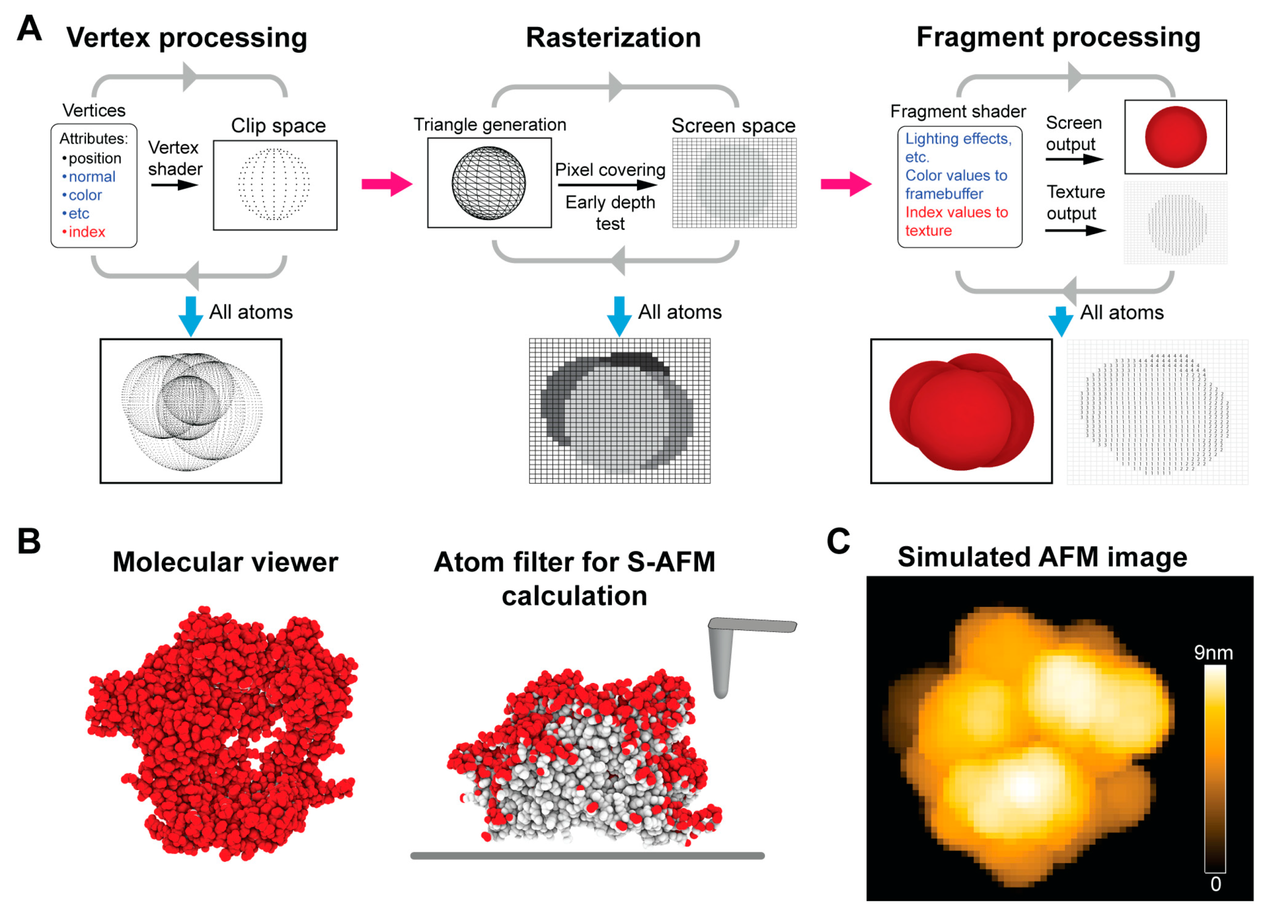
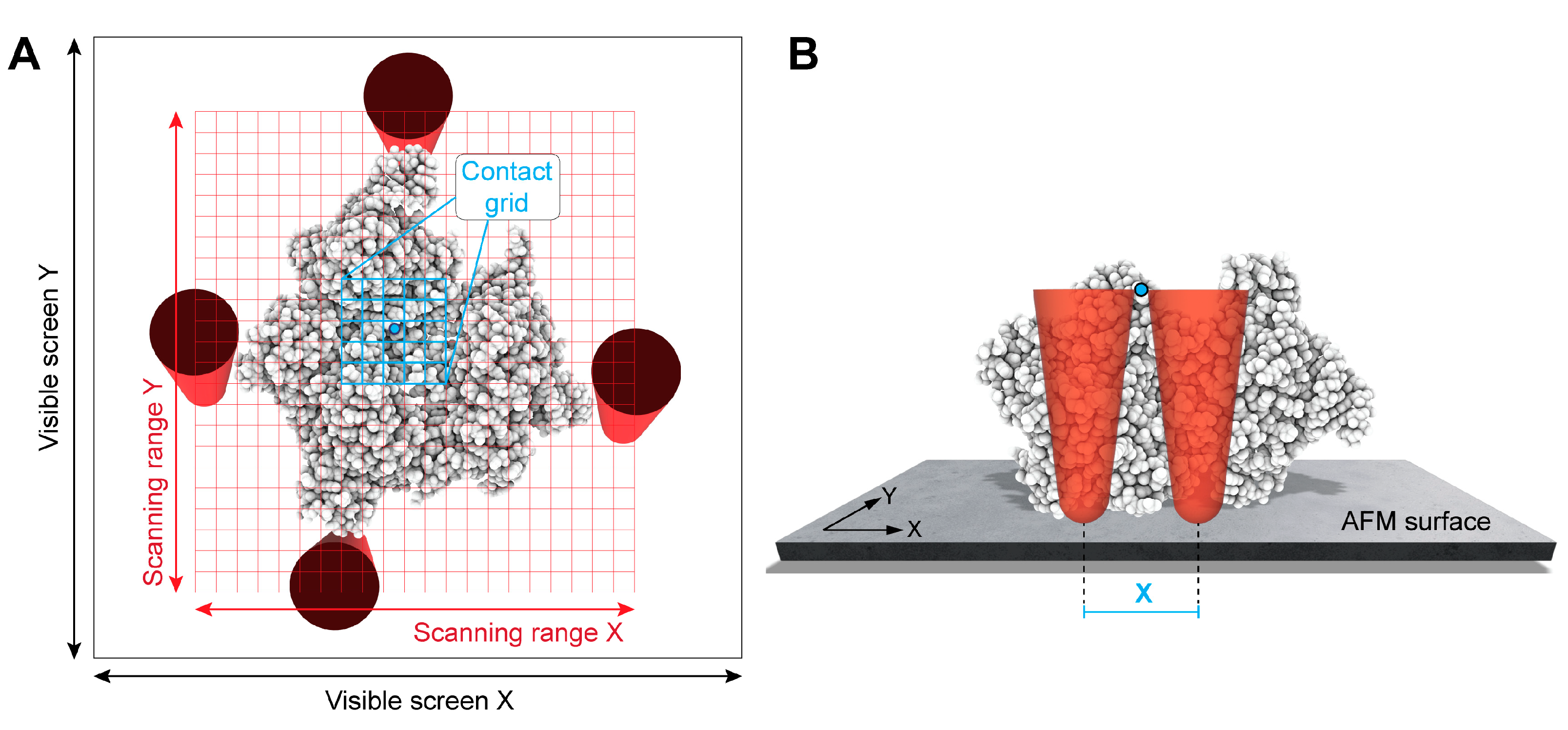
2.1. Primitive X-Y Filtering

We refer to primitive filtering as a selection method of relevant atoms in the horizontal and vertical (X, Y) scanning directions. For any arbitrary orientation of the biomolecular structure within the fixed screen canvas, first the tip scanning grid is obtained by determining the farthest possible tip contacts with the atomistic structure in the east and west directions (scanning range X), and those in the south and north directions (scanning range Y). We provide an illustration in Figure 1. The size of grid cells corresponds to the given scan step. As a next step, it would be reasonable to consider each individual grid cell with the tip placed at its center and calculate the tip contacts with all the atoms to select the largest height value of the structure relative to the AFM substrate.

We replace this generally inefficient procedure by looping just once over all the atoms instead. For each atom, a contact grid which covers the (X, Y) area from which the tip can touch this atom is determined as a sub-grid of the scanning grid (Figure 1). Its size apparently depends on the tip shape geometry and the distance of the atom to the AFM substrate. Then, for each cell of the contact grid, the collision height of the tip with this atom is computed (see Ref. [22] for details) and compared with previous height values computed from a tip collision with other atoms, always storing the larger height value. Thus, after looping over all the atoms, each cell of the scanning grid is assigned a single value which represents the sample height relative to the AFM substrate, as resulting from a convolution of the tip shape with the biomolecular surface. Simulated AFM using only primitive X-Y filtering (we refer to as the XY-F method) is obviously still highly inefficient.

Nonetheless, we will later apply this method simply to demonstrate the supremacy of the more sophisticated filtering method and computation of simulated AFM described next.

2.2. GPU-Based Lateral Z Direction Filtering of Surface Atoms

We developed an efficient method to filter the surface atoms in the lateral Z direction (i.e., in the vertical scanning direction of a biomolecular structure) based on graphics processing unit (GPU) computations. The underlying idea is that for any arbitrary 3D molecular orientation of a biomolecular structure, the set of atoms which are directly exposed to the scanning tip and can potentially come into contact with it contains exactly those which are displayed by rendering the corresponding graphical 2D view.

To visualize objects on the computer screen, graphic cards work with vertices and primitives. A primitive is the smallest unit used to build geometrical forms. Four main primitives are generally used: points, lines, triangles, and quads. To visualize atoms of a biomolecular structure as spheres (with corresponding Van der Waals radii) we use triangles as primitives. Spheres are therefore represented by a set of triangles, each of them having three vertices with attributes such as spatial position (x, y, z), orientation normal vector, color, etc.

In the first step, the GPU processes all vertices with their attributes via the vertex shader [23,24] (Figure 2A). The vertex shader places the vertices relative to each other in the clip space, a GPU internal 3D coordinate system with coordinates ranging from −1 to 1 that can be viewed as a 3D version of what will become the visible screen. Vertices having clip coordinates beyond this range will be later clipped out of the scene. The vertex shader is programmable, and the programmer has full control of it. After processing all vertices, the GPU groups them to form the corresponding triangles in the clip space, and then proceeds with rasterization.

Rasterization is the process by which the GPU transforms the 3D clip space into what will become the visible screen space, i.e., a 2D canvas of pixels (Figure 2A). Rasterization consists of determining which pixels are covered by a particular triangle and generates so called fragments accordingly. A fragment is characterized by the 2D position of the pixel it belongs to, plus the attributes inherited from the vertices of the triangle including the interpolated clip space z-coordinate interpreted as the depth value of the fragment by the GPU. During the processing of all triangles, many fragments will obviously share the same pixel position. However, an early depth test allows us to compare the depth of a newly generated fragment with that of the current fragment for a given pixel position, keeping only the least deep fragment. In such a situation, the result of the rasterization process is a pixel grid which consists of filtered fragments, each fragment representing the least deep position for a given pixel.

Finally, all remaining fragments from the previous rasterization process undergo fragment shading to determine a color for the processed fragment (Figure 2A). The normal and color attributes are usually used to compute light effects, and the 4D output vector from the fragment shader (RGB values plus opacity) will be interpreted by the GPU as a color for a particular pixel. In the context of visualizing a biomolecular structure, completed fragment shading would result in rendering the Van der Waals representation on the computer screen (render to screen pathway). That is, for a given molecular orientation, only the visible atoms are displayed and separated from the hidden non-visible atoms. Obviously, this separation would exactly correspond to filtering the subset of atoms that would be accessible to the scanning tip in that particular 3D orientation. Since, similar to the vertex shader, the fragment shader is programmable, we are able to implement the desired atom filter algorithm for S-AFM. This is possible by bypassing the rendering process and directing the fragment shader output to a texture (render to texture pathway), which can be viewed as an off-screen grid of pixels that can be read on the central processing unit (CPU). Therefore, the atom filtering procedure for an arbitrary orientation of the biomolecular structure to facilitate the computation of the corresponding S-AFM image can be performed independently from visualizing the 3D molecular structure (Figure 2B).

Like in the XY-F method, simulated AFM calculations can now be performed using the largely reduced set of filtered atoms to obtain the simulated AFM image (Figure 2C). We refer to this method as the XYZ-F method, and evaluate its performance against the XY-F method and the ultimate method described next.

2.3. GPU-Based Computation of Simulated AFM Images

Finally, we developed a method which takes into account the filtered set of atoms to efficiently compute the simulated AFM image employing an adaptation of the GPU workflow described above. We refer to this method as the XYZ-F2 method.

The lateral Z direction filtering uses the normal rendering process of the graphic card to output the indices of visible atoms. The simulated AFM calculation method we developed manipulates the workflow of the GPU from its original purpose to let the GPU parallelize the calculations with a minimal coding effort and without having to handle problems related to parallel computations. That is, there is no need to code a complicated program for parallelization and to take care of all related problems (such as concurrency access).

For this method, each atom is represented by a point primitive with the 3D position and corresponding Van der Waals radius as attributes. The rendering texture corresponds to the scanning grid (Figure 1A, red grid) in which each cell represents one pixel. The vertex shader operates in the same way as during filtering, i.e., vertices (in this case points) are mapped onto the clip space. Before the rasterization, vertices are intercepted by the geometry shader. The geometry shader is an optional programmable shader which takes a primitive as an input and outputs one or more primitives (which can be of a different type from the input primitive). For our purpose, we employ the geometry shader to generate for each filtered atom the corresponding tip contact sub-grid (Figure 1A, blue grid). That is, for each point primitive used as the input, the shader generates as an output a quad primitive with the size and position of the tip contact sub-grid for the corresponding atom. During the rasterization process, the obtained quads are mapped onto the pixel screen space and fragments are generated. Each fragment encodes the (X, Y) pixel position and the attributes of the point primitive it originated from, i.e., the corresponding atom position (x, y, z) and Van der Waals radius. The early depth test is inactivated such as all generated fragments resulting from all previously filtered atoms will be processed by the fragment shader. Generally, many fragments with different attributes share the same pixel position. The fragment shader is used to compute for each fragment the contact height of the tip (located over the corresponding pixel position) and the corresponding atom with respect to the AFM substrate surface, and the obtained height values are stored in the texture. The depth test takes place at this stage, keeping for each pixel of the texture only the fragment with the largest height value. Hence, the resulting texture contains for each pixel the largest height value obtained from simulating the scanning of the atomistic biomolecular structure in an arbitrary 3D orientation relative to the fixed AFM surface with a cone-shaped tip over the scanning grid with a prescribed spacing according to the experimental scan step. The corresponding simulated AFM image is visualized by mapping height values to a given color scale and coloring all pixels accordingly (Figure 2C).

We remark here on the tip-shape geometry for simulated scanning. In the XY-F and XYZ-F atom filtering methods, the computation of simulated AFM images was not based on the GPU workflow, and corresponded to the computation applied in our previous work [18,22]. That is, collisions of the cone-shaped tip with a spherical probe sphere at its end (characterized by apex angle and sphere radius parameters) and the filtered set of atoms in the respective methods were evaluated to generate the simulated AFM image (see Ref. [22] for modeling the tip–atom collisions). For the GPU-based computation of simulated AFM images in the XYZ-F2 method, the GPU requires knowledge of the tip shape—at the stage of the geometry shader to generate the tip contact sub-grid for each atom, and for the fragment shader to compute the contact heights of the tip with respect to the AFM substrate. The two tip-shape parameters are provided to the shader as so-called uniform variables. They are sent from the CPU and read for each execution of the shader, i.e., for each vertex by the geometry shader and for each fragment by the fragment shader at the running time. This means that, if our method is applied in a recursive scheme which requires changing the tip geometry, the two parameters can be modified on the CPU without having to recompile the GPU shaders, which would delay computations.

3. Results

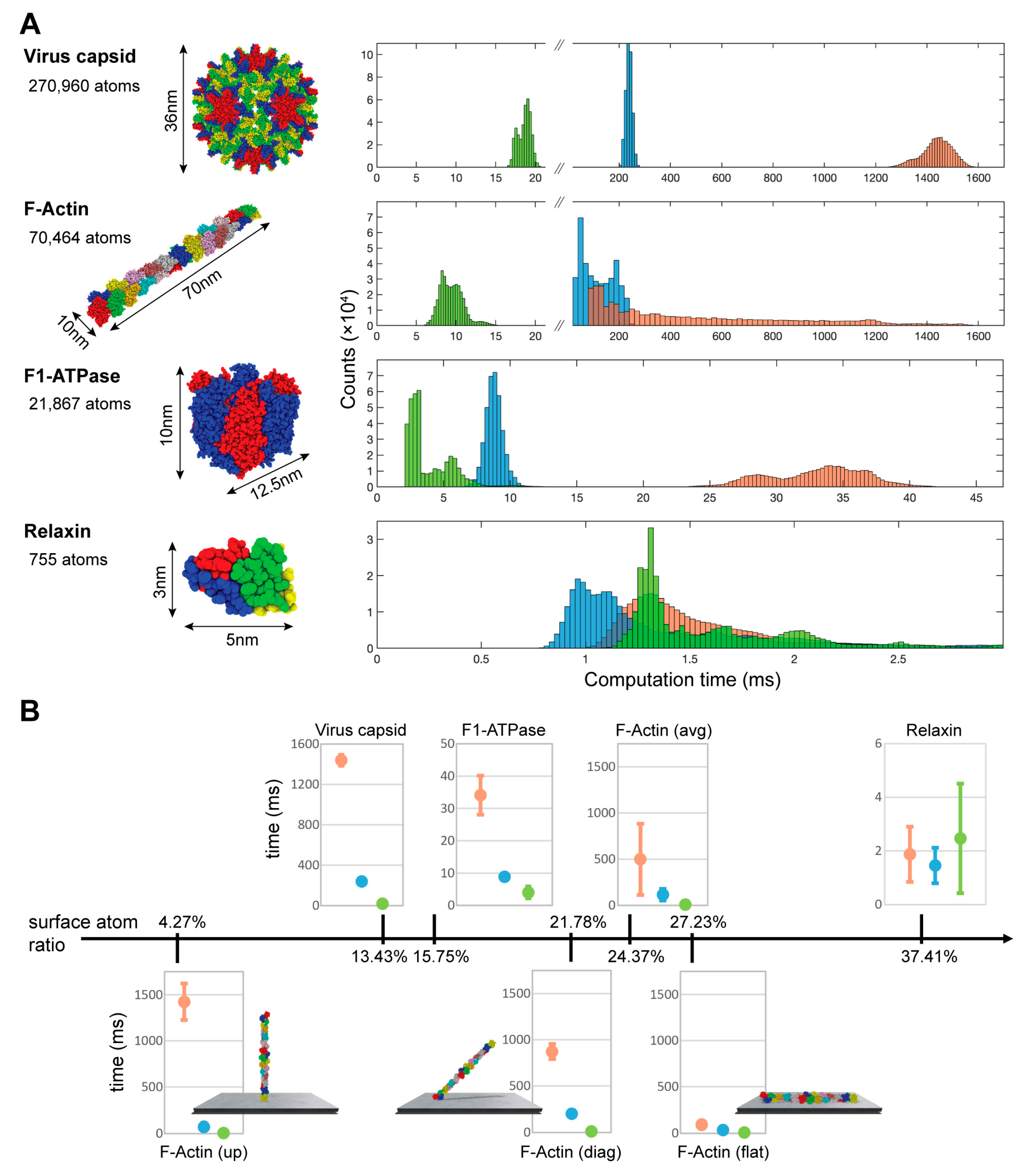
Quantification of the Computational Efficiency Gain

To quantify the efficiency gain of the developed atom-filtering methods and GPU calculations, we considered exhaustive sampling, which is a procedure employed during the fitting of structural data into AFM topographic images. This method samples rigid-body orientations of a given structural template in 3D space, each time computing the corresponding simulated AFM image, which is compared with an experimental target image. As structural templates, we used proteins which differ in size and shape:

• The hepatitis B virus capsid cryo-EM ball-shaped structure with a diameter of ~36 nm and a total of 270,960 atoms (constructed from PDB 6BVF);
• A model of the actin filament structure containing 24 subunits and having a rod-shape with ~10 nm diameter, ~70 nm length, and a total of 70,464 atoms (from Ref. [25]);
• The rotor-less F1-ATPase motor cube-like structure with lengths of ~10 and ~12.5 nm and a total of 21,867 atoms (PDB 1SKY);
• The small global-shaped relaxin protein with lengths of ~3 nm and ~5 nm with just 755 atoms (PDB 6RLX).

The molecular structures are shown in Figure 3A. For the four different protein structures, rigid-body orientations were sampled uniformly in 3D space along a grid with a 5 degree spacing, resulting in (360/5)³ = 373,248 conformations that were placed on a fixed plate and scanned in the lateral direction by the scanning tip across the XY scanning grid. For each orientation, we then recorded the computation time required to execute the filtering method and to calculate the corresponding simulated image (without visualizing it). We considered the three filtering methods described before, i.e., primitive XY filtering (XY-F), filtering including the lateral scanning direction Z (XYZ-F), and the latter with GPU calculations (XYZ-F2). The corresponding distributions of computation times for the four proteins are shown in Figure 3A and discussed below.

For the virus capsid structure, the calculation of an S-AFM image by the XYZ-F method (238 ± 12 ms) is faster than the XY-F method (1438 ± 61 ms) by a factor larger than 5 and is further enhanced by the XYZ-F2 method (19 ± 0.8 ms) by a factor larger than 10. To put those numbers into perspective, this means that the computation of S-AFM images during the rigid-body fitting of the capsid structure into an actual AFM image (with our chosen parameters and hardware setup) would on average take ~149 h (i.e., 6.2 days) using the inefficient XY-F methods, versus only ~2 h required with the XYZ-F2 implementation.

For the F-actin structure, the computation time of an S-AFM image by the XY-F method shows a very wide distribution (499 ± 386 ms), which is due to the special rod-shape of the molecule. For upright orientations with respect to the AFM substrate, the XY contact grid of the tip for each atom is generally large, because most atoms are located far from the substrate, hence resulting in a large number of tip–atom collisions to be calculated. In contrast, for orientations placed flat on the substrate, the XY contact grids of atoms have much smaller sizes, and computation is therefore faster. In such cases, speed improvements by additional Z-filtering are less relevant—distributions of the XY-F and XYZ-F methods even overlap—whereas, for filament positions oriented towards the upright shape, Z-filtering becomes increasingly important and the XYZ-F method significantly enhances the computation speed, as shown by the time distribution (117 ± 63 ms). The XYZ-F2 method supersedes others by improving the computation speed further by one order of magnitude (9.5 ± 1.5 ms).

For the relatively small F1-ATPase protein, the calculation of a simulated AFM image by the XYZ-F method (8.8 ± 0.7 ms) is faster than the XY-F method (34 ± 6 ms) by a factor of about four, and is further enhanced by the XYZ-F2 method (4 ± 2 ms) by a factor of about two. This means that the computation of S-AFM images during the rigid-body fitting of the F1 structure into an actual AFM image (with our chosen parameters and hardware setup) would on average take 212 min, versus only 25 min required with the XYZ-F2 implementation.

The results of the computation times obtained for the relaxin protein, i.e., (1.88 ± 1.03 ms) for the XY-F method, (1.46 ± 0.66 ms) for the XYZ-F method, and (2.47 ± 2.04 ms) for the XYZ-F2 method, clearly demonstrate the irrelevance of atom filtering for the simulated AFM of very small molecular structures.

The numerical investigations lead us to the following conclusions. Generally, our developed atom-filtering methods significantly speed up the calculation of simulated AFM images. The efficiency gain depends on the size and shape of proteins, and is apparently larger for cases in which the number of surface atoms is small, as compared to the total number of atoms. To clearly illustrate this aspect, we represent in Figure 3B the results discussed above, employing the ratio of surface atoms and all protein atoms as a coordinate. We emphasize again that for very large protein structures, the calculation time of a simulated AFM image can be reduced by about two orders of magnitude by the application of the developed filtering method. While, for proteins with typical sizes of ~10 nm, a significant speed up in calculation can be realized, the filtering methods become irrelevant for very small proteins with a generally larger surface atom ratio.

4. Discussion

The post-experimental analysis of biomolecular dynamics visualized by AFM experiments employing computational methods plays an increasingly important role. In this situation, simulated atomic force microscopy is the cornerstone method allowing us to correlate atomistic resolution biomolecular data with resolution-limited measured topographies.

The application of simulated AFM allows us to employ the enormous amount of available structural data, as well as data obtained from molecular dynamics simulations, to facilitate the interpretation of resolution-limited imaging towards an atomistic-level understanding of measured nanoscale processes. For example, rigid-body fitting by exhaustive sampling molecular orientations of a structural template [16,18], or flexible fitting methods resolving conformational changes [14,15,17], are based on the execution of simulated AFM in each iteration step towards finding the atomistic conformation that best matches with the target experimental AFM image. As we demonstrate, our developed method based on the GPU workflow can accelerate the computation of simulated AFM images by orders of magnitude, which can make a difference between several days versus a couple of hours required for fitting. Hence, this method will play an important role in computational analysis involving the calculations of simulated AFM (e.g., [26,27,28]), including expected applications in machine learning approaches.

We postulate that our developed method of atom filtering and the GPU-acceleration of simulated AFM images presents the algorithm of ultimate efficiency, and further efficiency gain can only be achieved by exploiting faster hardware. It would be interesting to further consider simulated AFM computations with more complex tip shape geometries. While, in this case, the calculation of tip–atom contacts will be more difficult, the presented atom-filtering algorithm and an adapted GPU-based computation are applicable.

The developed method is implemented in our BioAFMviewer software package for the simulated AFM of biomolecular structures and dynamics [22,29], where it allows for the visualization of biomolecular structures (of potentially massive sizes) combined with ultra-fast synchronized calculations and graphical representations of corresponding simulated AFM images (live simulated AFM).

References

1. Müller, D.J.; Dufrêne, Y.F. Atomic force microscopy as a multifunctional molecular toolbox in nanobiotechnology. Nat. Nanotech. 2008, 3, 261–269. [Google Scholar] [CrossRef] [PubMed]
2. Ando, T.; Uchihashi, T.; Scheuring, S. Filming biomolecular processes by high-speed atomic force microscopy. Chem. Rev. 2014, 114, 3120–3188. [Google Scholar] [CrossRef] [PubMed]
3. Ando, T. Directly watching biomolecules in action by high-speed atomic force microscopy. Biophys. Rev. 2017, 9, 421–429. [Google Scholar] [CrossRef] [PubMed]
4. Uchihashi, T.; Ganser, C. Recent advances in bioimaging with high-speed atomic force microscopy. Biophys. Rev. 2020, 12, 363–369. [Google Scholar] [CrossRef] [PubMed]
5. Casuso, I.; Redondo-Morata, L.; Rico, F. Biological physics by high-speed atomic force microscopy. Philos. Trans. R. Soc. A 2020, 378, 20190604. [Google Scholar] [CrossRef] [PubMed]
6. Ando, T. High-Speed Atomic Force Microscopy in Biology, 1st ed.; Springer: Berlin/Heidelberg, Germany, 2022; pp. 1–319. [Google Scholar] [CrossRef]
7. wwPDBconsortium. Protein data bank: The single global archive for 3D macromolecular structure data. Nucleic Acids Res. 2019, 47, D520–D528. [Google Scholar] [CrossRef] [PubMed]
8. Jumper, J.; Evans, R.; Pritzel, A.; Green, T.; Figurnov, M.; Ronneberger, O.; Tunyasuvunakool, K.; Bates, R.; Zidek, A.; Potapenko, A.; et al. Highly accurate protein structure prediction with AlphaFold. Nature 2021, 596, 583–589. [Google Scholar] [CrossRef] [PubMed]
9. Kenzaki, H.; Koga, N.; Hori, N.; Kanada, R.; Li, W.; Okazaki, K.; Yao, X.-Q.; Takada, S. CafeMol: A coarse-grained biomolecular simulator for simulating proteins at work. J. Chem. Theory Comput. 2011, 7, 1979–1989. [Google Scholar] [CrossRef]
10. Takada, S.; Kanada, R.; Tan, C.; Terakawa, T.; Li, W.; Kenzaki, H. Modeling structural dynamics of biomolecular complexes by coarse-grained molecular simulations. Acc. Chem. Res. 2015, 48, 3026–3035. [Google Scholar] [CrossRef]
11. Pak, A.J.; Voth, G.A. Advances in coarse-grained modeling of macromolecular complexes. Curr. Opin. Struct. Biol. 2018, 52, 119–126. [Google Scholar] [CrossRef]
12. Togashi, Y.; Flechsig, H. Coarse-grained protein dynamics studies using elastic network models. Int. J. Mol. Sci. 2018, 19, 3899. [Google Scholar] [CrossRef] [PubMed]
13. Flechsig, H.; Mikhailov, A.S. Simple mechanics of protein machines. J. R. Soc. Interface 2019, 16, 20190244. [Google Scholar] [CrossRef] [PubMed]
14. Niina, T.; Fuchigami, S.; Takada, S. Flexible fitting of biomolecular structures to atomic force microscopy images via biased molecular simulations. J. Chem. Theory Comput. 2020, 16, 1349–1358. [Google Scholar] [CrossRef] [PubMed]
15. Dasgupta, B.; Miyashita, O.; Tama, F. Reconstruction of low-resolution molecular structures from simulated AFM force microscopy images. Biochim. Biophys. Acta—Gen. Subj. 2020, 1864, 129420. [Google Scholar] [CrossRef]
16. Niina, T.; Matsunaga, Y.; Takada, S. Rigid-body fitting to atomic force microscopy images for inferring probe shape and biomolecular structure. PLoS Comput. Biol. 2021, 17, e1009215. [Google Scholar] [CrossRef]
17. Dasgupta, B.; Miyashita, O.; Uchihashi, T.; Tama, F. Reconstruction of three-dimensional conformations of bacterial ClpB from high-speed atomic-force-microscopy images. Front. Mol. Biosci. 2021, 8, 704274. [Google Scholar] [CrossRef]
18. Amyot, R.; Marchesi, A.; Franz, C.M.; Casuso, I.; Flechsig, H. Simulation atomic force microscopy for atomic reconstruction of biomolecular structures from resolution-limited experimental images. PLoS Comput. Biol. 2022, 18, e1009970. [Google Scholar] [CrossRef]
19. Ogane, T.; Noshiro, D.; Ando, T.; Yamashita, A.; Sugita, Y.; Matsunaga, Y. Development of hidden Markov modeling method for molecular orientations and structure estimation from high-speed atomic force microscopy time-series images. PLoS Comput. Biol. 2022, 18, e1010384. [Google Scholar] [CrossRef]
20. Flechsig, H.; Ando, T. Protein dynamics by the combination of high-speed AFM and computational modeling. Curr. Opin. Struct. Biol. 2023, 80, 102591. [Google Scholar] [CrossRef]
21. Owens, J.D.; Houston, M.; Luebke, D.; Green, S.; Stone, J.E.; Phillips, J.C. GPU computing. Proc. IEEE 2008, 96, 879–899. [Google Scholar] [CrossRef]
22. Amyot, R.; Flechsig, H. BioAFMviewer: An interactive interface for simulated AFM scanning of biomolecular structures and dynamics. PLoS Comput. Biol. 2020, 16, e1008444. [Google Scholar] [CrossRef] [PubMed]
23. Maughan, C.; Wloka, M. Vertex Shader Introduction; Technical report; NVIDIA Corporation: Santa Clara, CA, USA, 2001. [Google Scholar]
24. Ebner, M.; Reinhardt, M.; Albert, J. Evolution of vertex and pixel shaders. In Genetic Programming. EuroGP 2005. Lecture Notes in Computer Science; Keijzer, M., Tettamanzi, A., Collet, P., van Hemert, J., Tomassini, M., Eds.; Springer: Berlin/Heidelberg, Germany, 2005; Volume 3447. [Google Scholar] [CrossRef]
25. Pirani, A.; Vinogradova, M.V.; Curmi, P.M.G.; King, W.A.; Fletterick, R.J.; Craig, R.; Tobacman, L.S.; Xu, C.; Hatch, V.; Lehman, W. An atomic model of the thin filament in the relaxed and Ca2+-activated states. J. Mol. Biol. 2006, 357, 707–717. [Google Scholar] [CrossRef] [PubMed]
26. Fuchigami, S.; Niina, T.; Takada, S. Particle filter method to integrate high-speed atomic force microscopy measurements with biomolecular simulations. J. Chem. Theor. Comput. 2020, 16, 6609–6619. [Google Scholar] [CrossRef] [PubMed]
27. Fuchigami, S.; Niina, T.; Takada, S. Case report: Bayesian statistical interference of experimental parameters via biomolecular simulations: Atomic force microscopy. Front. Mol. Biosci. 2021, 8, 636940. [Google Scholar] [CrossRef]
28. Matsunaga, Y.; Fuchigami, S.; Ogane, T.; Takada, S. End-to-end differentiable blind tip reconstruction for noisy atomic force microscopy images. Sci. Rep. 2023, 13, 129. [Google Scholar] [CrossRef]
29. Amyot, R.; Kodera, N.; Flechsig, H. BioAFMviewer software for simulation atomic force microscopy of molecular structures and conformational dynamics. J. Struct. Biol. X 2023, 7, 100086. [Google Scholar] [CrossRef]
30. Kessenich, J.; Sellers, G.; Shreiner, D. OpenGL Programming Guide: The Official Guide to Learning OpenGL, Version 4.5 with SPIR-V; Addison-Wesley Professional: Glenview, IL, USA, 2016. [Google Scholar]
31. Rost, R.J.; Licea-Kane, B.; Ginsburg, D.; Kessenich, J.; Lichtenbelt, B.; Malan, H.; Weiblen, M. OpenGL Shading Language; Pearson Education: London, UK, 2009. [Google Scholar]
Figure 1. Primitive X-Y filtering. (A) The atomistic Van der Waals representation of a biomolecular structure is displayed in the scanning view perspective within the visible screen canvas (X, Y) outlined in black. The relevant scanning grid is shown in red, with the cell size corresponding to the given scan step. The four tip shapes illustrate the farthest possible tip contacts with the structure in the north, east, south, and west directions required to determine the scanning grid size. For a selected atom (blue circle), the computed tip contact grid is shown in blue. (B) The biomolecular structure is placed on the AFM substrate in a front view perspective. For a selected atom (blue circle), the contact range of a cone-shaped scanning tip is illustrated for the X direction.
Algorithms 17 00038 g001
Figure 2. GPU workflow for the lateral Z direction filtering of surface atoms. (A) For demonstration purposes, an example system of just five atoms is considered. Left, vertex processing: every vertex is placed in the clip space coordinate system by the vertex shader. Its attributes are transferred to the next step. The attributes used in classical rendering are written in blue. The attribute used in our filtering method, an index for tracking the atom, is written in red. Middle, rasterization: for each triplet of vertices, a triangle is formed, and fragments are generated based on the pixels covered by the triangle. The attributes of newly generated fragments result from the interpolation (or not) of the attributes of the three vertices. The depth test is applied to distinguish fragments in the front from others behind. Right, fragment processing: all fragments, which can now be viewed as pixels, enter the fragment shader. In classic rendering, the color is computed and rendered to the screen. In our filtering method, the index attribute of the fragment, inherited from the vertex of the atom covering this fragment, is written in a grid texture which can further be read on the CPU. The final grid texture contains, for each pixel, the tracking index of the atom closest to the viewer within this pixel position. (B) Left: molecular structure of the Cas9 endonuclease protein (from PDB 4OO8) in the scanning view perspective showing the atoms that are probed by the AFM scanning tip. Right: molecular structure in the front view perspective. The AFM substrate surface is indicated by the thick gray line. The surface atoms remaining after filtering (~24% of total atoms) are shown in red color. (C) Simulated AFM image for the scanning view in (B), computed from the set of filtered atoms.
Algorithms 17 00038 g002
Figure 3. Quantification of the computational efficiency gain by atom filtering methods. (A) Molecular structures of the investigated proteins are shown in the Van der Waals representation on the left side. The number of atoms is given, and their sizes are indicated. For each protein, distributions of the computation time required to execute the filtering method and to calculate the simulated AFM image for molecular orientations obtained from exhaustive sampling are shown as histograms for the XY-F (orange color), XYZ-F (blue color), and XYZ-F2 (green color) atom filtering methods on the right side. (B) The same results are represented, employing the surface atom ratio as a coordinate. For each filtering method, the data are shown as mean values and standard deviations of its computation time distribution (solid circle and error bar). For the upper row data (virus capsid, F1-ATPase, F-Actin (avg), relaxin), the surface atom ratio was obtained as an average of all considered molecular orientations. The bottom row data are for the actin filament considered in the upright, diagonal, and flat orientations with respect to the AFM substrate surface. For all plots of F-actin, data of the same scale were used for better comparisons.
Algorithms 17 00038 g003
Disclaimer/Publisher’s Note: The statements, opinions and data contained in all publications are solely those of the individual author(s) and contributor(s) and not of MDPI and/or the editor(s). MDPI and/or the editor(s) disclaim responsibility for any injury to people or property resulting from any ideas, methods, instructions or products referred to in the content.