
Hybrid Sparrow Search-Exponential Distribution Optimization with Differential Evolution for Parameter Prediction of Solar Photovoltaic Models

Abstract
1. Introduction
1.1. Motivations
1.2. Contributions
- ISSAEDO is a novel approach proposed to effectively identify the appropriate values for PV model parameters by enhancing the SSA and EDO algorithms using a DE technique and a bound-constraint adjustment procedure, which is defined accurately in Section 3.3.1 and Section 3.3.2.
- The DE technique is used to support diversity in populations and provide a comprehensive examination of the search space, thereby reducing the possibility of the ISSAEDO algorithm parallel to a local optimum.
- In order to establish the adequacy of the proposed ISSAEDO, the appropriate parameter values for two separate PV models, namely the SDM and the DDM, are specified.
- The ISSAEDO algorithm is assessed using recognized and competitive methodologies for the estimation of unknown parameters in PV systems. The results illustrate the strength and accuracy of the ISSAEDO in acquiring the coefficients of PV models.
1.3. Structure
2. PV Model Modeling and Problem Formulation
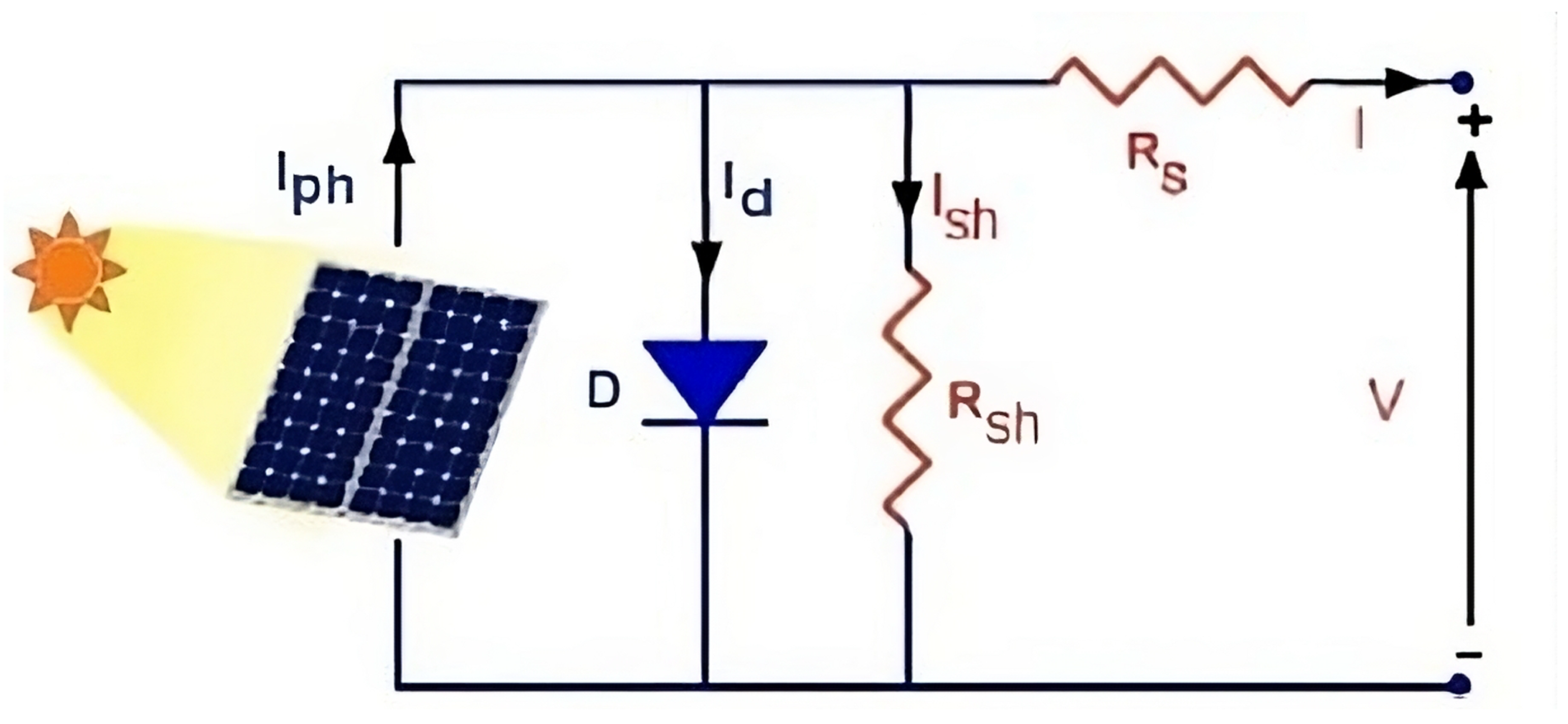
- SDM: The I-V characteristics of a PV cell or module are commonly described by a widely employed and uncomplicated model. The proposed model includes a single diode to represent the current passage through the PV cell or module, joining other elements such as series and shunt resistances.
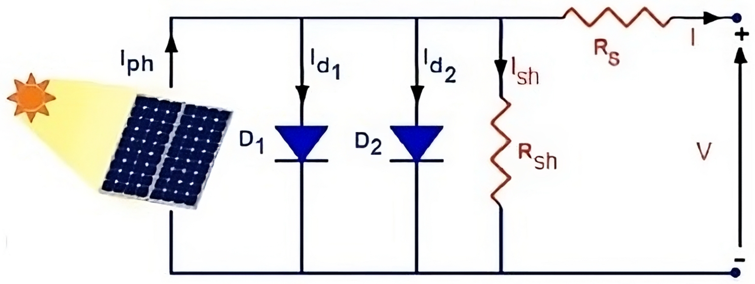
- DDM: The proposed expansion involves the integration of a second diode through the SDM system, which aims to reduce the negative impacts of recombination losses occurring in the PV cell or module. In various experimental conditions, the model has the capability to generate predictions of the I-V characteristic with enhanced accuracy.
- Analytical models: The behavior of PV systems is described by mathematical formulas in these models. These models can be utilized for the purpose of analyzing and enhancing the operational efficiency of PV systems.
- Empirical models: The models are derived from empirical data and can be utilized for approximating the performance of PV systems. In cases where there is an absence of comprehensive information related to the PV system, these models are commonly used.
- Computational models: Numerical approaches are employed to simulate the behavior of PV systems. These models have the capability of predicting and enhancing the efficiency of PV systems across a variety of situations.
2.1. Solar Cells
2.1.1. SDM Modelling
2.1.2. DDM Modelling
2.2. PV Models’ Objective Function
3. Proposed Improved Hybrid SSA with an EDO (ISSAEDO) Algorithm
3.1. Sparrow Search Algorithm (SSA)
- Exploration: In order to discover novel solutions, sparrows execute random examinations of the search space.
- Exploitation: Some sparrows display an ability to implement and modify the most optimal solutions currently available, with the aim of enhancing their performance.
- Memory: Each separate sparrow possesses the ability to identify its own optimal location as well as the most advantageous one identified by the whole group up until that point.
- Learning: Sparrows demonstrate adaptive behavior by changing their space position according to their memory and the optimal position determined by the collective behavior of the swarm.
- Designers often perform as very active reserves, providing explorers with access to gathering sites or instruction. Their primary responsibility is to identify regions characterized by significant food resources. The measurement of an individual’s fitness levels is used to evaluate the level of their energy reserves.
- Upon perceiving the presence of an attacker, sparrows immediately initiate a series of chirping expressions, working as an immediate warning signal. In case the alarm boundary exceeds the established safety limits, it is important for the producers to immediately instruct all hunters to relocate to a secure location.
- The potential for a sparrow to change into a producer function is dependent on its ability to actively search for suitable food sources. However, it is important to note that regardless of individual variations, the overall proportion of producers and hunters within the sparrow population remains constant.
- The species of birds demonstrating the most increased energy levels would be classified as producers. Numerous individuals who experience starvation are inclined to travel to different areas to seek food as a means of locating a source of food.
- Scavengers exhibit an ability to leave behind the producer organism that offers the most optimal food resources during their seeking activities. Certain scavengers engage in continuous surveillance of producers and compete for resources, strategically positioning themselves to enhance their own survival rate.
- In response to a perceived threat, sparrows located at the periphery of the group exhibit rapid movement into a designated safe area, thereby assuming a more advantageous position. Conversely, sparrows situated within the core of the group display aimless wandering behavior, likely driven by their desire to maintain proximity to their fellow group members.
| Algorithm 1 The original SSA algorithm |
| Input: G—the maximum iterations —the number of producers —the number of scroungers —the alarm value n—the number of sparrows Output: —the comprehensive best position discovered while searching —the comprehensive best fitness discovered, which should be decreased
|
3.2. Exponential Distribution Optimization (EDO) Algorithm
- Inverse Transform Method: The CDF of an exponential distribution can be mathematically reversed to derive the corresponding quantile function, which serves as the fundamental principle for this approach. The quantile function is a mathematical tool that provides the value of a random variable at which a specified probability is surpassed. The quantile function for the exponential distribution can be expressed as , where p represents the probability and denotes the rate parameter. In order to generate a random number from an exponential distribution, the process involves generating a uniform random number, u, that falls within the range of 0 to 1. Subsequently, the inverse quantile function formula is applied to derive the corresponding exponential random variable. The aforementioned methodology has the potential to be extended indefinitely in order to generate a random set of numbers that adhere to exponential distribution.
- Box–Muller Transform: This approach is designed to produce random numbers from a normal distribution, but it can also be used to generate random numbers from exponential distribution.
- Acceptance–Rejection Method: The proposed approach involves the generation of random numbers from a less complex distribution, followed by a decision-making process where these numbers are accepted or rejected based on a comparison with the probability density function (PDF) of the exponential distribution. One commonly chosen alternative for a simpler distribution is uniform distribution.
- A pair of uniform random numbers is generated between 0 and 1.
- Exponential random variable x can be computed as .
- If formula holds, where represents the probability density function (PDF) of the exponential distribution and M is a constant such that for all values of x, then the value of x can be accepted as a random number generated from exponential distribution. Alternatively, if x does not meet the criteria, it should be discarded and the process should be repeated. The computing cost of the acceptance–rejection approach can be significant, particularly when the ratio of the probability density function (PDF) is high, where represents the PDF of the less complex distribution. Nevertheless, the utilization of this approach can prove beneficial in cases where the inverse transform method is either inapplicable or presents implementation challenges.
- The Box–Muller transform is a method used to generate a pair of independent standard normal random variables .
- Exponential random variable x can be computed as x = , where u = . If , then x can be accepted as a random number from exponential distribution. In the event that x does not meet the criteria, it is necessary to decline its acceptance and thereafter initiate the process again.
- Memoryless property: The memoryless property of exponential distribution indicates the probability that an event occurring is not influenced by the time passed since the previous event. This characteristic can prove advantageous in depicting situations characterized by random or randomly generated events, where the timing between these events has significance.
- Flexibility: Exponential distribution, being a continuous probability distribution, has the capability to imitate continuous variables. This is advantageous in cases where the optimization problem involves continuous variables, such as in certain machine learning models.
- Simple parameterization: Exponential distribution is characterized by simple parameterization consisting of a single parameter, namely the rate parameter. In specific optimization scenarios, the simplicity of this probability distribution can facilitate its handling when contrasted with more intricate distributions.
- Widely used: Exponential distribution is widely recognized as a prominent probability distribution that enjoys comprehensive comprehension among researchers and practitioners across several academic domains. This suggests that those seeking to implement this concept in their professional endeavors can access a considerable amount of scholarly literature and resources. Certainly, we provide additional advantages of exponential distribution.
- Probability density function: Exponential distribution possesses a readily comprehensible probability density function, rendering it amenable to statistical analysis. This approach can prove advantageous in the pursuit of analytical solutions, particularly in theoretical investigations or the development of novel algorithms.
- Computational efficiency: Exponential distribution is known for its rapid sampling and assessment capabilities, rendering it a valuable tool in simulation research and computational modeling. The inverse transform method is a technique that can be employed to generate samples from exponential distribution with low computational requirements.
- Parameter estimation: The MLE is a straightforward approach utilized to estimate the parameters of exponential distribution based on observed data. The utilization of real-world data believed to be derived from an exponential distribution can be advantageous as it facilitates the estimation of distribution parameters based on the data.
- Relationship to other distributions: Exponential distribution shows close relationships with other probability distributions, such as Gamma distribution and Weibull distribution. Exponential distribution can be utilized as a fundamental element in models that involve complex structures and incorporate several probability distributions.
- Initially, a collection of solutions is generated through a random process, encompassing a diverse spectrum of values. The search process can be described as having exponential distributions, which means that the positions of all solutions can be considered as random variables that follow exponential distribution.
- To replicate the memoryless characteristic, a matrix is created and initialized with the identical value as the initial population.
- By employing the exploratory and exploitative phases of the suggested approach, all solutions gradually converge towards the global optimum.
- During the exploitation phase, the memoryless matrix is employed to simulate the memoryless property. This property allows for previously generated solutions, regardless of their past, to serve as influential members in updating new solutions, thereby preserving their established knowledge. Consequently, the responses are categorized into two distinct groups: those deemed as winners and those classified as losers. Furthermore, the utilization of the mean, exponential rate, and variance of the exponential distribution is observed in several contexts. The victorious entity progresses toward the guiding solution in order to explore the global optimum in its vicinity, whereas the defeated entity travels toward the victorious entity.
- In order to enhance the exploration phase, the mean solution and two randomly chosen winners from the initial population are employed for the update process. The average response and variability exhibit significant deviation from the optimal global solution at the outset. The discrepancy between the average response and the universally optimal solution is progressively diminished through the process of optimization until it reaches a minimum value. The switch parameter mentioned above is employed with a probability of 0.5 to determine whether to execute the exploration phase or the exploitation phase.
- After being generated, the perimeter of each newly obtained solution is analyzed. The user’s responses are then stored in a matrix with no memory.
- The original population is updated by including new solutions obtained through the utilization of a greedy method during both exploitation and exploration stages. If the new solution proves to be successful, the original population undergoes updates. In the event that the newly proposed solution demonstrates efficacy, it results in the modification of the original population.
- After the conclusion of the optimization technique, it is observed that all of the solutions converge towards the global optimum solution. The anticipated values for the mean and variance of the optimal solution are expected to be low, while the value of the scale parameter is projected to be high.
| Algorithm 2 The original EDO algorithm |
| Input: N—the population size —the maximum time —the lower bound —the upper bound Output: —the optimal solutions obeying the exponential solution
|
3.3. Proposed Improved Hybrid SSA with the EDO (ISSAEDO) Algorithm
3.3.1. DE Technique
- Mutation stepThe objective of this procedure, alternatively referred to as a differential mutation, is to generate a mutated vector, for every solution vector in each iteration. The modified vector is generated by a random selection process, where three nominee vectors are chosen from a range of options ranging from 1 to population size. The process involves computing the difference between two of the selected nominee vectors, namely and , and afterward merging the obtained results. After multiplying the third nominee vector, Xr1, by a mutation weighting factor (W) within the interval [0, 1] [34], it is subsequently added to the aforementioned difference. The numerical expression for I is as follows:One distinguishing factor between DE and other evolutionary processes lies in this particular stage.
- Crossover stepTo ensure the preservation of population diversity, the DE technique use this particular phase to adapt the differential mutation search strategy. The offspring vector is generated using a crossover operation that combines values from the objective vector and the altered vector . Based on the principles of binomial and exponential operators, the prevailing and fundamental crossover search operators can be enumerated as follows:Random numbers are selected from the range , while rand is picked from the interval . This selection ensures that the modified vector will have at least one dimension. Variable , often assigned a high value , is the user-specified crossover rate that determines the probability of crossing over each element. A comparison is performed between variables and rand, as elucidated in Equation (20). If the value of rand is less than or equal to , then the calculation of is derived from the value of . If this condition is not met, infers .
- Selection stepThe final stage of the DE cycle is the selection phase. In this stage, the fitness function values of the offspring vector to the corresponding target vector are compared to determine the solution that is more appropriate for future iteration. The procedure for determining a winner is explained asIn the case where the fitness function, denoted as , generates a value lower than that of the target vector, , the offspring vector, , is reassigned to be equal to the target vector, . Alternatively, the previous target vector, denoted as , remains unchanged.
3.3.2. Bound-Constraint Adjustment Approach
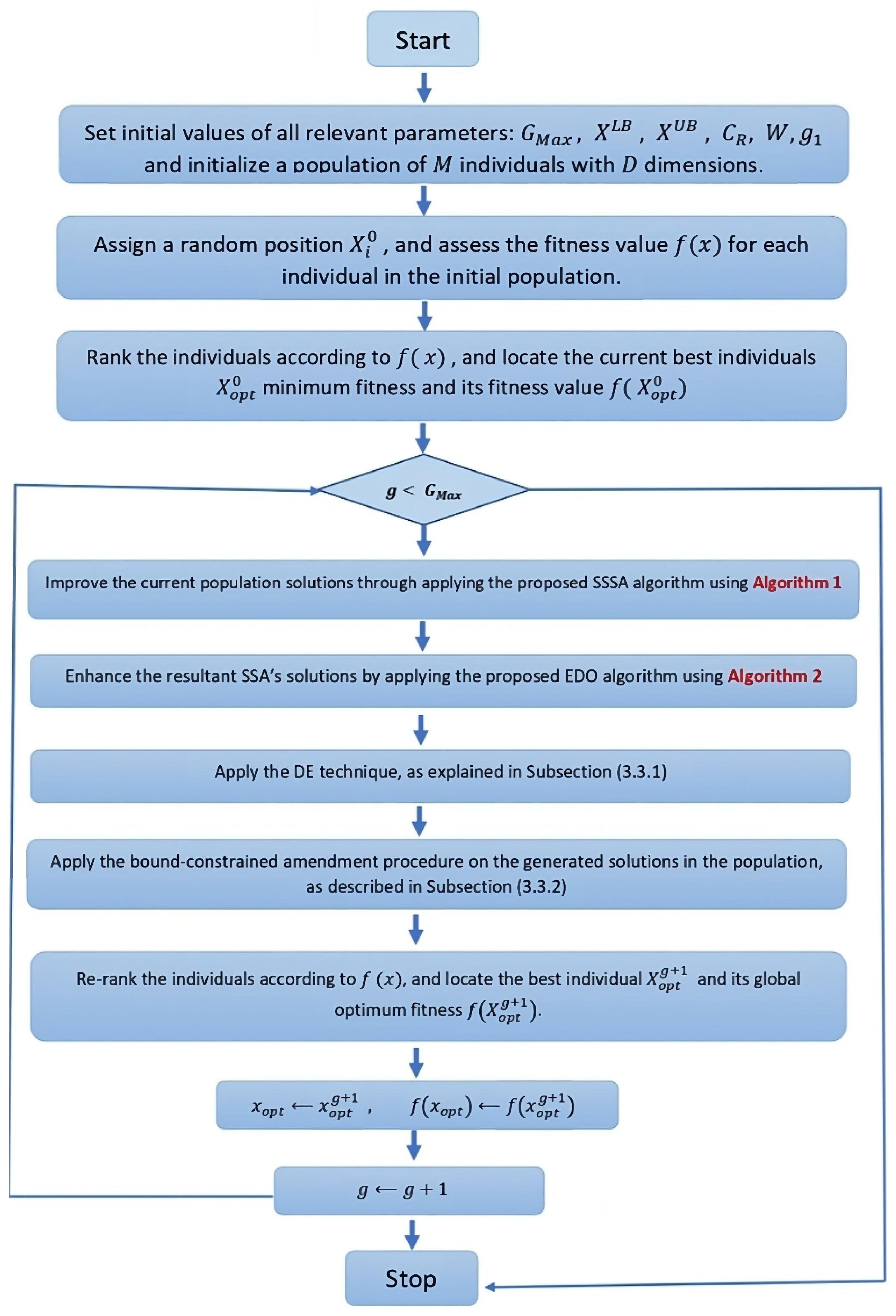
3.3.3. The Exhaustive ISSAEDO Algorithm
- The population of sparrow solutions with random values within the defined search space is initialized. Each solution represents a set of parameters for the solar PV model.
- The SSA component of the algorithm is responsible for the exploration and exploitation of the search space. It simulates the foraging behavior of sparrows to iteratively improve solutions.
- The sparrows move within the search space by adjusting their positions based on their current positions, the best solution found so far, and random exploration.
- The exploration phase allows the algorithm searching for new regions of the search space, while the exploitation phase focuses on intensifying the search around promising solutions.
- The EDO component utilizes the properties of the exponential distribution to optimize the parameters.
- The exponential distribution has a probability density function that can be used to model the likelihood of occurrence of events. In the context of optimization, it can guide the search towards regions that are more likely to contain optimal solutions.
- The EDO component incorporates the exponential distribution into the SSA framework to enhance the exploration and exploitation abilities of the algorithm.
- The algorithm adapts the parameters of exponential distribution, such as the rate parameter, during the optimization process to improve the convergence towards optimal solutions.
- The DE component is another optimization technique employed within the ISSAEDO algorithm.
- DE operates on a population of candidate solutions and iteratively improves them through a combination of mutation, recombination, and selection.
- During the DE phase, a set of new candidate solutions is generated by perturbing and recombining the existing solutions in the population.
- The new solutions are then compared with the original solutions, and selection is performed based on their fitness or objective function values.
- DE introduces additional variation and diversity into the optimization process, allowing for a more thorough exploration of the search space.
| Algorithm 3 ISSAEDO algorithm |
| Input: M—overall number of individuals (population size) —maximum number of iterations D—dimensions of individuals’ positions —lower bounds of individuals’ positions —upper bounds of individuals’ positions —crossover rate W—weighting factor Output: —the global optimum position discovered while searching —the best fitness discovered, which should be decreased
|

3.4. Computational Complexity of the ISSAEDO Algorithm
- Population initialization
- Position upgrading
- Random Position Amendment
- Appreciation of fitness function
- DE strategy
- M is the population size.
- is the maximum number of iterations.
- is the time complexity for the single solution evaluation.
- assumed that the SSA algorithm per iteration is a standard which is this one.
- assumed the same for the EDO algorithm.
- assumed the same for the EDO algorithm per iteration as well.
4. PV Models Results and Experimental Analysis
- Memetic Adaptive DE (MADE) Algorithm [4];
- Differential Evolution (DE) method with an adaptation approach (SaDE) [36];
- DE with an ensemble of parameters and mutation strategies (EPSDE) [37];
- DE with composite trial vector generation strategies (CoDE) [38];
- A Multi-Population Ensemble DE (MPEDE) [39];
- An Enhanced adaptive DE method with population adaptation strategy (jDE) [40];
- Adaptive DE with optional external Archive (JADE) [41];
- A Performance Guided JAYA (PGJAYA) [42];
- An enhanced JAYA (IJAYA) [43];
- Multiple Learning Backtracking Search Approach (MLBSA) [44].
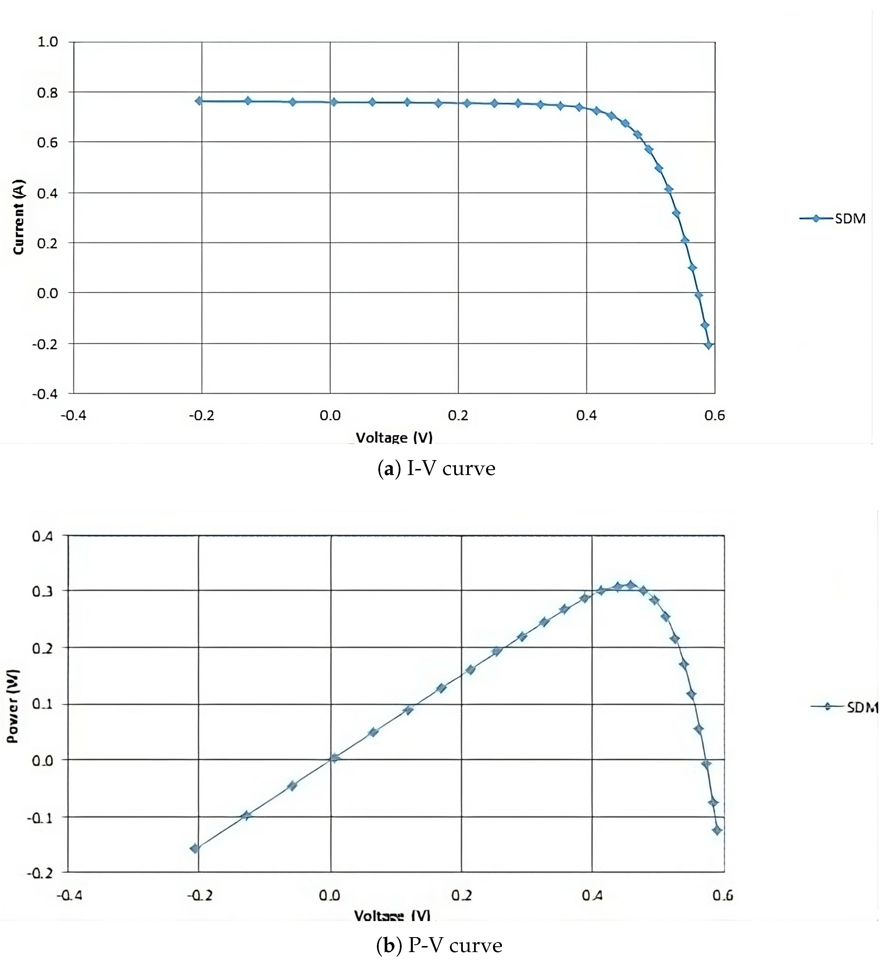
4.1. SDM Results
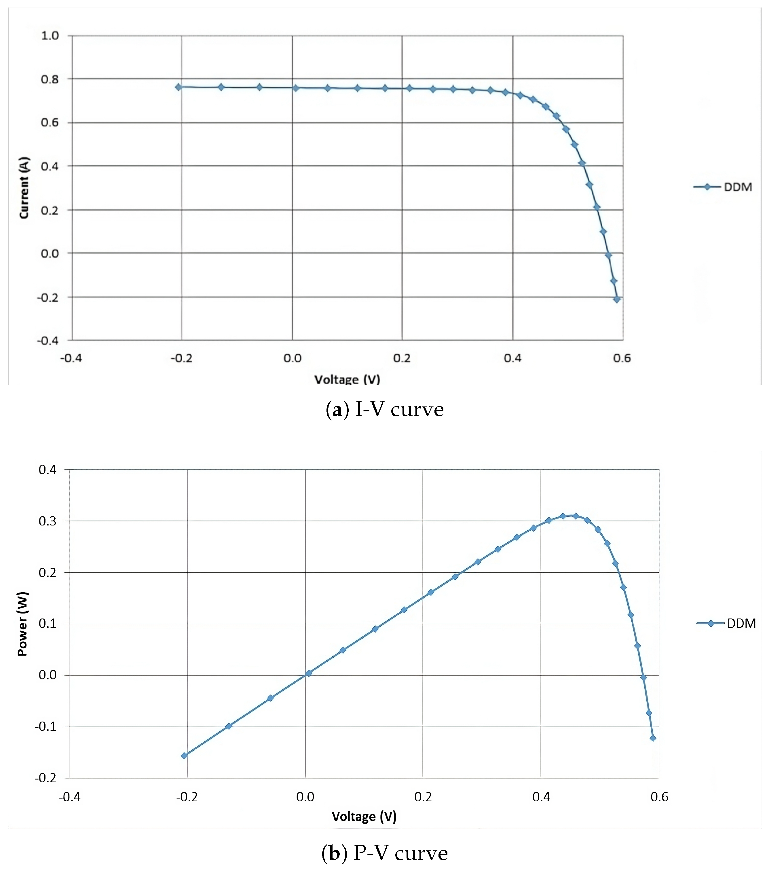
4.2. DDM Results
4.3. Various ISSAEDO’s Components Results
4.4. Results of the Proposed ISSAEDO Compared with Other Recent Algorithms
5. Discussion
6. Conclusions and Future Work
Author Contributions
Funding
Data Availability Statement
Conflicts of Interest
References
- Mahajan, M.; Kumar, S.; Pant, B.; Khan, R. Improving Accuracy of Air Pollution Prediction by Two Step Outlier Detection. In Proceedings of the 2021 International Conference on Advances in Electrical, Computing, Communication and Sustainable Technologies (ICAECT), Bhilai, India, 19–20 February 2021; pp. 1–7. [Google Scholar]
- Hosenuzzaman, M.; Rahim, N.A.; Selvaraj, J.; Hasanuzzaman, M.; Malek, A.A.; Nahar, A. Global prospects, progress, policies, and environmental impact of solar photovoltaic power generation. Renew. Sustain. Energy Rev. 2015, 41, 284–297. [Google Scholar] [CrossRef]
- Parida, B.; Iniyan, S.; Goic, R. A review of solar photovoltaic technologies. Renew. Sustain. Energy Rev. 2011, 15, 1625–1636. [Google Scholar] [CrossRef]
- Li, S.; Gong, W.; Yan, X.; Hu, C.; Bai, D.; Wang, L.; Gao, L. Parameter extraction of photovoltaic models using an improved teaching-learning-based optimization. Energy Convers. Manag. 2019, 186, 293–305. [Google Scholar] [CrossRef]
- Li, S.; Gong, W.; Gu, Q. A comprehensive survey on meta-heuristic algorithms for parameter extraction of photovoltaic models. Renew. Sustain. Energy Rev. 2021, 141, 110828. [Google Scholar] [CrossRef]
- Moustafa, G. Parameter Identification of Solar Photovoltaic Systems Using an Augmented Subtraction-Average-Based Optimizer. Eng 2023, 4, 1818–1836. [Google Scholar] [CrossRef]
- Abd El-Mageed, A.A.; Abohany, A.A.; Saad, H.M.; Sallam, K.M. Parameter extraction of solar photovoltaic models using queuing search optimization and differential evolution. Appl. Soft Comput. 2023, 134, 110032. [Google Scholar] [CrossRef]
- Sallam, K.M.; Hossain, M.A.; Chakrabortty, R.K.; Ryan, M.J. An improved gaining-sharing knowledge algorithm for parameter extraction of photovoltaic models. Energy Convers. Manag. 2021, 237, 114030. [Google Scholar] [CrossRef]
- Nassar-Eddine, I.; Obbadi, A.; Errami, Y.; Agunaou, M. Parameter estimation of photovoltaic modules using iterative method and the Lambert W function: A comparative study. Energy Convers. Manag. 2016, 119, 37–48. [Google Scholar] [CrossRef]
- Phang, J.; Chan, D.; Phillips, J. Accurate analytical method for the extraction of solar cell model parameters. Electron. Lett. 1984, 10, 406–408. [Google Scholar] [CrossRef]
- Chan, D.S.; Phang, J.C. Analytical methods for the extraction of solar-cell single-and double-diode model parameters from IV characteristics. IEEE Trans. Electron. Devices 1987, 34, 286–293. [Google Scholar] [CrossRef]
- Saloux, E.; Teyssedou, A.; Sorin, M. Explicit model of photovoltaic panels to determine voltages and currents at the maximum power point. Sol. Energy 2011, 85, 713–722. [Google Scholar] [CrossRef]
- Sera, D.; Teodorescu, R.; Rodriguez, P. Photovoltaic module diagnostics by series resistance monitoring and temperature and rated power estimation. In Proceedings of the 2008 34th Annual Conference of IEEE Industrial Electronics, Orlando, FL, USA, 10–13 November 2008; pp. 2195–2199. [Google Scholar]
- Bai, J.; Liu, S.; Hao, Y.; Zhang, Z.; Jiang, M.; Zhang, Y. Development of a new compound method to extract the five parameters of PV modules. Energy Convers. Manag. 2014, 79, 294–303. [Google Scholar] [CrossRef]
- Batzelis, E.I.; Papathanassiou, S.A. A method for the analytical extraction of the single-diode PV model parameters. IEEE Trans. Sustain. Energy 2015, 7, 504–512. [Google Scholar] [CrossRef]
- Li, S.; Gong, W.; Yan, X.; Hu, C.; Bai, D.; Wang, L. Parameter estimation of photovoltaic models with memetic adaptive differential evolution. Sol. Energy 2019, 190, 465–474. [Google Scholar] [CrossRef]
- Di Piazza, M.C.; Vitale, G. Photovoltaic Sources: Modeling and Emulation; Springer: Berlin/Heidelberg, Germany, 2013. [Google Scholar]
- Gottschalg, R.; Rommel, M.; Infield, D.G.; Kearney, M. The influence of the measurement environment on the accuracy of the extraction of the physical parameters of solar cells. Meas. Sci. Technol. 1999, 10, 796. [Google Scholar] [CrossRef]
- Jiang, L.L.; Maskell, D.L.; Patra, J.C. Parameter estimation of solar cells and modules using an improved adaptive differential evolution algorithm. Appl. Energy 2013, 112, 185–193. [Google Scholar] [CrossRef]
- Li, S.; Gu, Q.; Gong, W.; Ning, B. An enhanced adaptive differential evolution algorithm for parameter extraction of photovoltaic models. Energy Convers. Manag. 2020, 205, 112443. [Google Scholar] [CrossRef]
- Kharchouf, Y.; Herbazi, R.; Chahboun, A. Parameter’s extraction of solar photovoltaic models using an improved differential evolution algorithm. Energy Convers. Manag. 2022, 251, 114972. [Google Scholar] [CrossRef]
- Hu, Z.; Gong, W.; Li, S. Reinforcement learning-based differential evolution for parameters extraction of photovoltaic models. Energy Rep. 2021, 7, 916–928. [Google Scholar] [CrossRef]
- Farah, A.; Belazi, A.; Benabdallah, F.; Almalaq, A.; Chtourou, M.; Abido, M. Parameter extraction of photovoltaic models using a comprehensive learning Rao-1 algorithm. Energy Convers. Manag. 2022, 252, 115057. [Google Scholar] [CrossRef]
- Wolpert, D.H.; Macready, W.G. No free lunch theorems for optimization. IEEE Trans. Evol. Comput. 1997, 1, 67–82. [Google Scholar] [CrossRef]
- Abd El-Mageed, A.A.; Gad, A.G.; Sallam, K.M.; Munasinghe, K.; Abohany, A.A. Improved binary adaptive wind driven optimization algorithm-based dimensionality reduction for supervised classification. Comput. Ind. Eng. 2022, 167, 107904. [Google Scholar] [CrossRef]
- Nelson, J.A. The Physics of Solar Cells; World Scientific Publishing Company: Singapore, 2003. [Google Scholar]
- Rusirawan, D.; Farkas, I. Identification of model parameters of the photovoltaic solar cells. Energy Procedia 2014, 57, 39–46. [Google Scholar] [CrossRef]
- Chen, X.; Yu, K. Hybridizing cuckoo search algorithm with biogeography-based optimization for estimating photovoltaic model parameters. Sol. Energy 2019, 180, 192–206. [Google Scholar] [CrossRef]
- Li, L.; Xiong, G.; Yuan, X.; Zhang, J.; Chen, J. Parameter extraction of photovoltaic models using a dynamic self-adaptive and mutual-comparison teaching-learning-based optimization. IEEE Access 2021, 9, 52425–52441. [Google Scholar] [CrossRef]
- Diachenko, O.; Dobrozhan, O.; Opanasyuk, A.; Ivashchenko, M.; Protasova, T.; Kurbatov, D.; Čerškus, A. The influence of optical and recombination losses on the efficiency of thin-film solar cells with a copper oxide absorber layer. Superlattices Microstruct. 2018, 122, 476–485. [Google Scholar] [CrossRef]
- Gao, X.; Cui, Y.; Hu, J.; Xu, G.; Yu, Y. Lambert W-function based exact representation for double diode model of solar cells: Comparison on fitness and parameter extraction. Energy Convers. Manag. 2016, 127, 443–460. [Google Scholar] [CrossRef]
- Xue, J.; Shen, B. A novel swarm intelligence optimization approach: Sparrow search algorithm. Syst. Sci. Control Eng. 2020, 8, 22–34. [Google Scholar] [CrossRef]
- Storn, R.; Price, K. Differential evolution–a simple and efficient heuristic for global optimization over continuous spaces. J. Glob. Optim. 1997, 11, 341–359. [Google Scholar] [CrossRef]
- Sallam, K.M.; Elsayed, S.M.; Sarker, R.A.; Essam, D.L. Improved united multi-operator algorithm for solving optimization problems. In Proceedings of the 2018 IEEE Congress on Evolutionary Computation (CEC), Rio de Janeiro, Brazil, 8–13 July 2018; pp. 1–8. [Google Scholar]
- Easwarakhanthan, T.; Bottin, J.; Bouhouch, I.; Boutrit, C. Nonlinear minimization algorithm for determining the solar cell parameters with microcomputers. Int. J. Sol. Energy 1986, 4, 1–12. [Google Scholar] [CrossRef]
- Qin, A.K.; Huang, V.L.; Suganthan, P.N. Differential evolution algorithm with strategy adaptation for global numerical optimization. IEEE Trans. Evol. Comput. 2008, 13, 398–417. [Google Scholar] [CrossRef]
- Mallipeddi, R.; Suganthan, P.N.; Pan, Q.K.; Tasgetiren, M.F. Differential evolution algorithm with ensemble of parameters and mutation strategies. Appl. Soft Comput. 2011, 11, 1679–1696. [Google Scholar] [CrossRef]
- Wang, Y.; Cai, Z.; Zhang, Q. Differential evolution with composite trial vector generation strategies and control parameters. IEEE Trans. Evol. Comput. 2011, 15, 55–66. [Google Scholar] [CrossRef]
- Tong, L.; Dong, M.; Jing, C. An improved multi-population ensemble differential evolution. Neurocomputing 2018, 290, 130–147. [Google Scholar] [CrossRef]
- Yang, M.; Cai, Z.; Li, C.; Guan, J. An improved adaptive differential evolution algorithm with population adaptation. In Proceedings of the 15th Annual Conference on Genetic and Evolutionary Computation, New York, NY, USA, 6–10 July 2013; pp. 145–152. [Google Scholar]
- Zhang, J.; Sanderson, A.C. JADE: Adaptive differential evolution with optional external archive. IEEE Trans. Evol. Comput. 2009, 13, 945–958. [Google Scholar] [CrossRef]
- Yu, K.; Qu, B.; Yue, C.; Ge, S.; Chen, X.; Liang, J. A performance-guided JAYA algorithm for parameters identification of photovoltaic cell and module. Appl. Energy 2019, 237, 241–257. [Google Scholar] [CrossRef]
- Yu, K.; Liang, J.; Qu, B.; Chen, X.; Wang, H. Parameters identification of photovoltaic models using an improved JAYA optimization algorithm. Energy Convers. Manag. 2017, 150, 742–753. [Google Scholar] [CrossRef]
- Yu, K.; Liang, J.; Qu, B.; Cheng, Z.; Wang, H. Multiple learning backtracking search algorithm for estimating parameters of photovoltaic models. Appl. Energy 2018, 226, 408–422. [Google Scholar] [CrossRef]
- Abdel-Basset, M.; Mohamed, R.; Chakrabortty, R.K.; Sallam, K.; Ryan, M.J. An efficient teaching-learning-based optimization algorithm for parameters identification of photovoltaic models: Analysis and validations. Energy Convers. Manag. 2021, 227, 113614. [Google Scholar] [CrossRef]
- Abdel-Basset, M.; El-Shahat, D.; Sallam, K.M.; Munasinghe, K. Parameter extraction of photovoltaic models using a memory-based improved gorilla troops optimizer. Energy Convers. Manag. 2022, 252, 115134. [Google Scholar] [CrossRef]
- Liang, J.; Qiao, K.; Yu, K.; Ge, S.; Qu, B.; Xu, R.; Li, K. Parameters estimation of solar photovoltaic models via a self-adaptive ensemble-based differential evolution. Sol. Energy 2020, 207, 336–346. [Google Scholar] [CrossRef]
- Yang, X.; Gong, W. Opposition-based JAYA with population reduction for parameter estimation of photovoltaic solar cells and modules. Appl. Soft Comput. 2021, 104, 107218. [Google Scholar] [CrossRef]
- Li, S.; Gong, W.; Wang, L.; Yan, X.; Hu, C. A hybrid adaptive teaching–learning-based optimization and differential evolution for parameter identification of photovoltaic models. Energy Convers. Manag. 2020, 225, 113474. [Google Scholar] [CrossRef]


| Parameter | SDM | DDM |
|---|---|---|
| Type | Poly-crystalline | Poly-crystalline |
| Number of cells in zeros | 1 | 1 |
| Number of cells in parallel | 1 | 1 |
| Size | 57 mm diameter | 57 mm diameter |
| Test temperature (T) | 33 C | 33 C |
| Parameter | SDM/DDM | |
|---|---|---|
| LB | UB | |
| 0 | 1 | |
| , , () | 0 | 1 |
| 0 | 0.5 | |
| 0 | 100 | |
| , , | 1 | 2 |
| Parameter | SDM | DDM |
|---|---|---|
| 12,000 | 25,000 |
| Algorithm | (A) | (A) | RMSE | |||
|---|---|---|---|---|---|---|
| ISSAEDO | 0.7607755300 | 0.3230207850 | 0.0363770930 | 53.7185252000 | 1.4811835800 | 9.8602187789E-04 |
| MADE | 0.7607755332 | 0.3230000000 | 0.0363770930 | 53.7185005600 | 1.4811835853 | 9.8602187789E-04 |
| SaDE | 0.7606306974 | 0.3881272938 | 0.0356323074 | 59.7703987550 | 1.4998983522 | 9.8767260000E-04 |
| EPSDE | 0.7607755303 | 0.3230208010 | 0.0363770928 | 53.7185218340 | 1.4811835873 | 9.8602190000E-04 |
| CoDE | 0.7606228498 | 0.3630150610 | 0.0358942084 | 57.1533115200 | 1.4930535768 | 1.0143800000E-03 |
| MPEDE | 0.7607800000 | 0.3230200000 | 0.0363770000 | 53.7190000000 | 1.4812000000 | 9.8602190000E-04 |
| jDE | 0.7607755293 | 0.3230073030 | 0.0363772593 | 53.7178992130 | 1.4811793730 | 9.8602190000E-04 |
| JADE | 0.7607772391 | 0.3249853860 | 0.0363544613 | 54.0345027540 | 1.4817918886 | 9.8626910000E-04 |
| PGJAYA | 0.7607719946 | 0.3206643324 | 0.0364105809 | 53.6010407450 | 1.4804454483 | 9.8615000000E-04 |
| IJAYA | 0.7607138662 | 0.3176309309 | 0.0364462526 | 53.6012765710 | 1.4794893522 | 9.8737780000E-04 |
| MLBSA | 0.7607764255 | 0.3230719859 | 0.0363765964 | 53.7177979230 | 1.4811995702 | 9.8602210000E-04 |
| Algorithm | RMSE | |||
|---|---|---|---|---|
| Minimum | Maximum | Mean | STD | |
| ISSAEDO | 9.8602188E-04 | 9.8602188E-04 | 9.8602188E-04 | 1.7950565E-14 |
| MADE | 9.8602188E-04 | 9.8602191E-04 | 9.8602189E-04 | 6.4252315E-12 |
| SaDE | 9.8767260E-04 | 1.8884850E-03 | 1.1952670E-03 | 2.0847960E-04 |
| EPSDE | 9.8602190E-04 | 1.3563180E-03 | 1.0257090E-03 | 8.3009550E-05 |
| CoDE | 1.0143800E-03 | 1.2244620E-03 | 1.1046240E-03 | 5.8656380E-05 |
| MPEDE | 9.8602190E-04 | 9.8602190E-04 | 9.8602190E-04 | 4.3589640E-12 |
| jDE | 9.8602190E-04 | 1.4239390E-03 | 1.1186400E-03 | 1.2769220E-04 |
| JADE | 9.8626910E-04 | 1.1812090E-03 | 1.0460130E-03 | 5.3216160E-05 |
| PGJAYA | 9.8615000E-04 | 1.4631150E-03 | 1.0607400E-03 | 1.0901850E-04 |
| IJAYA | 9.8737780E-04 | 1.5932340E-03 | 1.1949590E-03 | 2.0842070E-04 |
| MLBSA | 9.8602210E-04 | 1.2345460E-03 | 1.0561590E-03 | 7.9342520E-05 |
| Algorithm | (A) | (A) | (A) | RMSE | ||||
|---|---|---|---|---|---|---|---|---|
| ISSAEDO | 0.7607810790 | 0.2259739760 | 0.0367404315 | 55.4854436000 | 1.4510166600 | 0.7493498910 | 2.0000000000 | 9.8248485179E-04 |
| MADE | 0.7607810797 | 0.2260000000 | 0.0367404211 | 55.4854055726 | 1.4510173879 | 0.7493000000 | 1.9999999997 | 9.8248485587E-04 |
| SaDE | 0.7605529097 | 0.4019423717 | 0.0352812892 | 63.8865930751 | 1.5048179780 | 0.1090051418 | 1.9074684965 | 9.8458640000E-04 |
| EPSDE | 0.7607839281 | 0.7398515250 | 0.0367635704 | 55.4482499718 | 1.9812650310 | 0.2200262130 | 1.4489316075 | 9.8272390000E-04 |
| CoDE | 0.7606657463 | 0.7169618000 | 0.0359843956 | 56.2001315362 | 1.8307575470 | 0.3482198660 | 1.4889528267 | 1.0104260000E-03 |
| MPEDE | 0.7607800000 | 0.7493400000 | 0.0367400000 | 55.4850000000 | 2.0000000000 | 0.2259700000 | 1.4510000000 | 9.8248490000E-04 |
| jDE | 0.7608080110 | 0.2262055410 | 0.0367193581 | 55.2789940264 | 1.4513068866 | 0.7028794990 | 1.9818923230 | 9.8285900000E-04 |
| JADE | 0.7607724100 | 0.1939047400 | 0.0365249693 | 54.2950340976 | 1.7341490459 | 0.2446544550 | 1.4607843563 | 9.8519020000E-04 |
| PGJAYA | 0.7607837732 | 0.4630972107 | 0.0367145383 | 55.3345161445 | 1.7858272830 | 0.1849328798 | 1.4386695529 | 9.8525850000E-04 |
| IJAYA | 0.7607756123 | 0.4719030929 | 0.0366006720 | 55.1172649192 | 1.9439093713 | 0.2468714629 | 1.4589209674 | 9.8343310000E-04 |
| MLBSA | 0.7607813802 | 0.2375023013 | 0.0366501347 | 54.9172957588 | 1.4558677128 | 0.4640968779 | 1.9157161435 | 9.8348930000E-04 |
| Algorithm | RMSE | |||
|---|---|---|---|---|
| Minimum | Maximum | Mean | STD | |
| ISSAEDO | 9.8248485E-04 | 9.8602238E-04 | 9.8408156E-04 | 1.4185686E-06 |
| MADE | 9.8248486E-04 | 9.8910305E-04 | 9.8511840E-04 | 1.8182667E-06 |
| SaDE | 9.8458640E-04 | 1.7089030E-03 | 1.2130700E-03 | 1.9964670E-04 |
| EPSDE | 9.8272390E-04 | 2.5031770E-03 | 1.5854020E-03 | 4.5970190E-04 |
| CoDE | 1.0104260E-03 | 1.7836150E-03 | 1.3436560E-03 | 1.9219140E-04 |
| MPEDE | 9.8248490E-04 | 9.8673210E-04 | 9.8461020E-04 | 1.4732270E-06 |
| jDE | 9.8285900E-04 | 1.6377260E-03 | 1.0650130E-03 | 1.5496370E-04 |
| JADE | 9.8519020E-04 | 2.8240180E-03 | 1.6014520E-03 | 4.4163080E-04 |
| PGJAYA | 9.8525850E-04 | 1.4380610E-03 | 1.0345370E-03 | 8.8557680E-05 |
| IJAYA | 9.8343310E-04 | 1.7581600E-03 | 1.1920610E-03 | 2.0934500E-04 |
| MLBSA | 9.8348930E-04 | 1.0282400E-03 | 9.9315490E-04 | 1.3358040E-05 |
| Algorithm | (A) | (A) | RMSE | |||
|---|---|---|---|---|---|---|
| SSA | 0.7611237070 | 0.2553533450 | 0.0372915872 | 46.3936672000 | 1.4578304200 | 1.1351825925E-03 |
| EDO | 0.1494502860 | 0.6416363660 | 0.2519534990 | 85.2178070000 | 1.4772455100 | 8.7962970619E-03 |
| SSAEDO | 0.9631364110 | 0.0491793204 | 0.2857274100 | 79.7732647000 | 1.3100563200 | 1.5303729578E-03 |
| DE | 0.7607755300 | 0.3230207970 | 0.0363770928 | 53.7185230000 | 1.4811835900 | 9.8602187789E-04 |
| SSADE | 0.7607755240 | 0.3230210790 | 0.0363770907 | 53.7186219000 | 1.4811836700 | 9.8602187790E-04 |
| EDODE | 0.3842538840 | 0.0994869333 | 0.1675509700 | 65.4048061000 | 1.0850875100 | 9.9793333516E-04 |
| ISSAEDO | 0.7607755300 | 0.3230207850 | 0.0363770930 | 53.7185252000 | 1.4811835800 | 9.8602187789E-04 |
| Algorithm | RMSE | |||
|---|---|---|---|---|
| Minimum | Maximum | Mean | STD | |
| SSA | 1.1351826E-03 | 4.9923896E-02 | 1.6412148E-02 | 1.2306843E-02 |
| EDO | 8.7962971E-03 | 4.9100913E-02 | 2.6817953E-02 | 1.0819581E-02 |
| SSAEDO | 1.5303730E-03 | 1.4939081E-02 | 4.3928599E-03 | 3.2682416E-03 |
| DE | 9.8602188E-04 | 9.8634410E-04 | 9.8603281E-04 | 5.7814328E-08 |
| SSADE | 9.8602188E-04 | 1.3052765E-03 | 1.0047413E-03 | 5.7919392E-05 |
| EDODE | 9.9793333E-04 | 1.7105545E-02 | 3.2587436E-03 | 3.8058891E-03 |
| ISSAEDO | 9.8602188E-04 | 9.8602188E-04 | 9.8602188E-04 | 1.7950565E-14 |
| Algorithm | (A) | (A) | (A) | RMSE | ||||
|---|---|---|---|---|---|---|---|---|
| SSA | 0.7607292070 | 0.0962466377 | 0.0335449530 | 66.7972347000 | 1.8260237200 | 0.6065940090 | 1.5498233600 | 1.8536310762E-03 |
| EDO | 0.3920021250 | 0.1988300750 | 0.2727070710 | 96.9255478000 | 1.2826811200 | 0.1131069910 | 1.8711319500 | 6.5929103094E-03 |
| SSAEDO | 0.7607600010 | 0.4846699400 | 0.0360174473 | 63.7180802000 | 1.5358508900 | 0.0024107608 | 1.2508950300 | 1.2588395188E-03 |
| DE | 0.7607818090 | 0.2236078160 | 0.0367528712 | 55.5095539000 | 1.4501308800 | 0.7684338980 | 1.9999712500 | 9.8248876571E-04 |
| SSADE | 0.7607811140 | 0.2259500230 | 0.0367405577 | 55.4853989000 | 1.4510077100 | 0.7495405350 | 1.9999999800 | 9.8248485256E-04 |
| EDODE | 0.7607741680 | 0.1465861030 | 0.0363745501 | 53.7224790000 | 1.4883549700 | 0.1771543740 | 1.4760443000 | 9.8602722237E-04 |
| ISSAEDO | 0.7607810790 | 0.2259739760 | 0.0367404315 | 55.4854436000 | 1.4510166600 | 0.7493498910 | 2.0000000000 | 9.8248485179E-04 |
| Algorithm | RMSE | |||
|---|---|---|---|---|
| Minimum | Maximum | Mean | STD | |
| SSA | 1.8536311E-03 | 3.1783778E-02 | 7.9238393E-03 | 6.3513919E-03 |
| EDO | 6.5929103E-03 | 4.0223204E-02 | 2.3216000E-02 | 9.0087144E-03 |
| SSAEDO | 1.2588395E-03 | 1.0135373E-02 | 3.5780324E-03 | 1.9048191E-03 |
| DE | 9.8248877E-04 | 9.8608817E-04 | 9.8496762E-04 | 1.1333581E-06 |
| SSADE | 9.8248485E-04 | 9.8948889E-04 | 9.8552284E-04 | 1.5032988E-06 |
| EDODE | 9.8602722E-04 | 8.8772632E-03 | 2.8693984E-03 | 2.1017978E-03 |
| ISSAEDO | 9.8248485E-04 | 9.8602238E-04 | 9.8408156E-04 | 1.4185686E-06 |
| Algorithm | (A) | (A) | RMSE | |||
|---|---|---|---|---|---|---|
| ISSAEDO | 0.7607755300 | 0.3230207850 | 0.0363770930 | 53.7185252000 | 1.4811835800 | 9.8602187789E-04 |
| IGSK | 0.760775530000 | 0.323000000000 | 0.036377092600 | 53.718525318300 | 1.481183592100 | 9.8602187789E-04 |
| MTLBO | 0.760775530000 | 0.323000000000 | 0.036377090000 | 53.718525100000 | 1.481183590000 | 9.8602190000E-04 |
| MIGTO | 0.760775529978 | 0.323020838966 | 0.036377092476 | 53.718529820618 | 1.481183599063 | 9.8602187789E-04 |
| DERL | 0.760775530476 | 0.323020835362 | 0.036377092315 | 53.718526836059 | 1.481183597903 | 9.8602187789E-04 |
| SEDE | 0.760918670367 | 0.342699806830 | 0.036159060560 | 54.374637365047 | 1.487135632586 | 9.8602419564E-04 |
| EJAYA | 0.760775530234 | 0.323020820235 | 0.036377092603 | 53.718527449147 | 1.481183593200 | 9.8602187789E-04 |
| ATLDE | 0.766113038531 | 0.976041045494 | 0.028905212893 | 35.699281625311 | 1.606957864299 | 5.0558093207E-03 |
| Algorithm | RMSE | ||||
|---|---|---|---|---|---|
| Minimum | Maximum | Mean | STD | CPU Time (s) | |
| ISSAEDO | 9.8602188E-04 | 9.8602188E-04 | 9.8602188E-04 | 1.7950565E-14 | |
| IGSK | 9.86021880E-04 | 9.86021880E-04 | 9.86021880E-04 | 3.5821018E-17 | 5.34 |
| MTLBO | 9.8602190E-04 | 9.8602190E-04 | 9.8602190E-04 | 1.9092749E-17 | — |
| MIGTO | 9.86021880E-04 | 9.86021880E-04 | 9.86021880E-04 | 1.4800000E-17 | 3.15 |
| DERL | 9.86021880E-04 | 9.86021880E-04 | 9.86021880E-04 | 7.7778590E-17 | 2.89 |
| SEDE | 9.8602420E-04 | 1.0460447E-03 | 9.9286093E-04 | 1.2097805E-05 | 2.51 |
| EJAYA | 9.86021880E-04 | 9.86021880E-04 | 9.86021880E-04 | 3.5158347E-13 | 10.26 |
| ATLDE | 5.0558093E-03 | 2.6010278E-02 | 1.2918977E-02 | 3.8927359E-03 | 0.69 |
| Algorithm | (A) | (A) | (A) | RMSE | ||||
|---|---|---|---|---|---|---|---|---|
| ISSAEDO | 0.7607810790 | 0.2259739760 | 0.0367404315 | 55.4854436000 | 1.4510166600 | 0.7493498910 | 2.0000000000 | 9.8248485179E-04 |
| IGSK | 0.760781078800 | 0.749300000000 | 0.036740428600 | 55.485434254300 | 2.000000000000 | 0.226000000000 | 1.451016892800 | 9.8248485179E-04 |
| MTLBO | 0.760781000000 | 0.749300000000 | 0.036740430000 | 55.485447000000 | 1.999999900000 | 0.225970000000 | 1.451016000000 | 9.8248490000E-04 |
| MIGTO | 0.760781079716 | 0.225974098430 | 0.036740429798 | 55.485441004589 | 1.451016706890 | 0.749349388682 | 1.999999999997 | 9.8248485179E-04 |
| DERL | 0.760781427162 | 0.769331473053 | 0.036755411997 | 55.511061446498 | 1.999999885032 | 0.223397967779 | 1.450045266267 | 9.8249599338E-04 |
| SEDE | 0.759974384717 | 0.521351239996 | 0.033000678297 | 64.299061995503 | 1.579409410340 | 0.167338150195 | 1.841165682244 | 9.8262738626E-04 |
| EJAYA | 0.760786512297 | 0.230273700314 | 0.036721466099 | 55.329778672223 | 1.452584868825 | 0.711749061850 | 1.999999965157 | 9.8249988436E-04 |
| ATLDE | 0.766288413557 | 0.762958757469 | 0.026086596318 | 33.403749313859 | 1.630211622282 | 0.991549225520 | 1.719109201673 | 3.2186265367E-03 |
| Algorithm | RMSE | ||||
|---|---|---|---|---|---|
| Minimum | Maximum | Mean | STD | CPU Time (s) | |
| ISSAEDO | 9.8248485E-04 | 9.8602238E-04 | 9.8408156E-04 | 1.4185686E-06 | |
| IGSK | 9.8248485E-04 | 9.86021880E-04 | 9.8272774E-04 | 8.9578942E-06 | 14.08 |
| MTLBO | 9.8250260E-04 | 9.8248490E-04 | 9.8248550E-04 | 3.3000000E-09 | — |
| MIGTO | 9.8266170E-04 | 9.8602187E-04 | 9.8266170E-04 | 7.7100000E-06 | 5.32 |
| DERL | 9.8249600E-04 | 1.0091744E-03 | 9.8634733E-04 | 4.4372558E-06 | 3.82 |
| SEDE | 9.8262739E-04 | 1.1069935E-03 | 1.0092765E-03 | 3.9080194E-05 | 0.22 |
| EJAYA | 9.8249988E-04 | 9.8613006E-04 | 9.9057738E-04 | 1.7720444E-06 | 12.02 |
| ATLDE | 3.2186265E-03 | 1.4438034E-02 | 7.9795069E-03 | 2.9918516E-03 | 1.38 |
Disclaimer/Publisher’s Note: The statements, opinions and data contained in all publications are solely those of the individual author(s) and contributor(s) and not of MDPI and/or the editor(s). MDPI and/or the editor(s) disclaim responsibility for any injury to people or property resulting from any ideas, methods, instructions or products referred to in the content. |
© 2024 by the authors. Licensee MDPI, Basel, Switzerland. This article is an open access article distributed under the terms and conditions of the Creative Commons Attribution (CC BY) license (https://creativecommons.org/licenses/by/4.0/).
Share and Cite
Abd El-Mageed, A.A.; Al-Hamadi, A.; Bakheet, S.; Abd El-Rahiem, A.H. Hybrid Sparrow Search-Exponential Distribution Optimization with Differential Evolution for Parameter Prediction of Solar Photovoltaic Models. Algorithms 2024, 17, 26. https://doi.org/10.3390/a17010026
Abd El-Mageed AA, Al-Hamadi A, Bakheet S, Abd El-Rahiem AH. Hybrid Sparrow Search-Exponential Distribution Optimization with Differential Evolution for Parameter Prediction of Solar Photovoltaic Models. Algorithms. 2024; 17(1):26. https://doi.org/10.3390/a17010026
Chicago/Turabian StyleAbd El-Mageed, Amr A., Ayoub Al-Hamadi, Samy Bakheet, and Asmaa H. Abd El-Rahiem. 2024. "Hybrid Sparrow Search-Exponential Distribution Optimization with Differential Evolution for Parameter Prediction of Solar Photovoltaic Models" Algorithms 17, no. 1: 26. https://doi.org/10.3390/a17010026
APA StyleAbd El-Mageed, A. A., Al-Hamadi, A., Bakheet, S., & Abd El-Rahiem, A. H. (2024). Hybrid Sparrow Search-Exponential Distribution Optimization with Differential Evolution for Parameter Prediction of Solar Photovoltaic Models. Algorithms, 17(1), 26. https://doi.org/10.3390/a17010026