Machine Learning Model for Multiomics Biomarkers Identification for Menopause Status in Breast Cancer

Abstract

Identifying menopause-related breast cancer biomarkers is crucial for enhancing diagnosis, prognosis, and personalized treatment at that stage of the patient’s life. In this paper, we present a comprehensive framework for extracting multiomics biomarkers specifically related to breast cancer incidence before and after menopause. Our approach integrates DNA methylation, gene expression, and copy number alteration data using a systematic pipeline encompassing data preprocessing and handling class imbalance, dimensionality reduction, and classification. The framework starts with MutSigCV for data preprocessing and ensuring data quality. The Synthetic Minority Over-sampling Technique (SMOTE) up-sampling technique is applied to address the class imbalance representation. Then, Principal Component Analysis (PCA) transforms the DNA methylation, gene expression, and copy number alteration data into a latent space. The purpose is to discard irrelevant variations and extract relevant information. Finally, a classification model is built based on the transformed multiomics data into a unified representation. The framework contributes to understanding the complex interplay between menopause and breast cancer, thereby revealing more precise diagnostic and therapeutic strategies in the future. The explainable artificial intelligence model Shapley based on the XGBoost regressor showed the power of the selected gene expressions for predicting the menopause status, and the potential biomarkers included RUNX1, PTEN, MAP3K1, and CDH1. The literature confirmed the findings.

1. Introduction

Breast cancer stands as a prominent global health challenge, thus causing substantial morbidity and mortality among women worldwide [1]. Female breast cancer has surpassed lung cancer as the most commonly diagnosed cancer by 11.7%, with an estimated 2.3 million new cases [2]. The intricate interplay between menopause, a natural biological event marking the cessation of reproductive function, and breast cancer has garnered increasing attention due to its profound impact on disease incidence, progression, and therapeutic responses [3,4]. The transition through menopause brings about complex physiological changes, including hormonal fluctuations, metabolic shifts, and alterations in immune function. These changes, in turn, influence the behavior of breast cancer and its response to therapeutic interventions [5]. Vincent suggested that in women with breast cancer, menopause and its associated symptoms can have substantial negative effects on both quality of life and long-term health. These menopausal symptoms may arise through different scenarios: (1) natural menopause coinciding with a breast cancer diagnosis; (2) the reappearance of symptoms after discontinuing hormone replacement therapy; and (3) menopause induced by cancer treatments such as chemotherapy, ovarian ablation/suppression, and adjuvant endocrine therapy [6]. Several studies have analyzed breast cancer menopausal status [7,8]. In a study involving 167 invasive cancers from postmenopausal women undergoing exclusive endocrine therapy, the expression of ERα and ERβ1 was examined. Specifically, 143 cases received adjuvant Tamoxifen following surgery. The analysis, conducted through immunohistochemistry and reverse transcription RT–PCR, revealed a strong correlation between ERα protein expression and the corresponding RNA detected using RT–PCR (chi-squared test, $p<$ 0.001). However, ERβ1 protein and mRNA exhibited inconsistency in their association [7]. In another postmenopause breast cancer study, Crujeiras et al. reported that the epigenome of breast tumors is affected by a complex interaction between the body mass index (BMI) and the menopausal status [8]. In this study, we identify different multiomics activities between premenopause and postmenopause breast cancer patients.

The advancement of high-throughput multiomics technologies, encompassing genomics, transcriptomics, proteomics, and metabolomics, has ushered in a new era of cancer research. These innovative tools enable comprehensive profiling of the molecular landscape of breast cancer, thereby facilitating the discovery of molecular signatures that are intricately linked to disease dynamics, prognosis, and treatment outcomes. Consequently, there is a growing recognition of the potential of multiomics data in uncovering biomarkers that hold promise for enhancing the diagnosis and management of breast cancer [9], particularly within the context of menopausal status [10]. The convergence of multiomics data and advanced computational methodologies presents an opportunity for a holistic exploration of the complex interplay between molecular alterations, menopause, and breast cancer. Through the integration of data across diverse omics domains, researchers can unravel novel insights into the molecular mechanisms underlying the intricate relationship between menopause and breast cancer.

The primary objective of this paper is to harness the wealth of multiomics data to identify biomarkers that are capable of distinguishing menopause status within the realm of breast cancer. By leveraging the power of multiomics integration, we aim to unveil the molecular intricacies of this crucial life transition and its implications for breast cancer dynamics. Through rigorous analysis and the interpretation of multiomics data, we endeavor to uncover molecular signatures that not only illuminate the intersection of menopause and breast cancer but also hold potential as diagnostic, prognostic, and therapeutic markers.

In the subsequent sections, we delve into the methodologies applied, the multiomic dataset, and the outcomes achieved in pursuit of our overarching goal. The methodology consists of handling feature selection to handle the curse of dimensionality of having thousands of features for hundreds of samples.

The dataset was split into premenopause versus postmenopause samples, where the number of postmenopause samples was way more than the premenopause ones. This leads to an imbalanced class problem. This challenge was handled through an up-sampling technique. The dimensionality reduction techniques were used to transfer the various types of data into linear transformation before merging them into one prediction model. Our aspiration is that the insights presented herein will contribute to a deeper understanding of the molecular underpinnings of breast cancer in the context of menopause. Furthermore, we hope these insights will open new avenues for personalized strategies in diagnosing and treating breast cancer.

2. Related Work

Dimensionality reduction techniques were used to study the omics data in menopause within the context of breast cancer [11,12]. Egelston applied t-distributed Stochastic Neighbor Embedding (t-SNE) on single-cell RNA sequencing of CD8+ T cells from 10 premenopausal patients. The t-SNE approach identified four unbiased Seurat clusters [11]. Treelet transform (TT) derived nutrient patterns from dietary questionnaires involving twenty-three log-transformed nutrient densities. TT is a complementary method to PCA in nutritional epidemiology as it produces readily interpretable sparse components. The study assessed the association between quintiles of nutrient pattern scores and breast cancer (BC) risk, thereby considering overall BC risk, as well as hormonal receptor and menopausal status, by utilizing hazard ratios (HRs) and 95% confidence intervals via Cox proportional hazards models [12].

Embedding has been proposed to integrate multiomics data for cancer outcome prediction [9,13]. These techniques are used heavily in processing nonlinear embedding methods, including t-SNE [14] and Pairwise Controlled Manifold Approximation Projection (PaCMAP) [15]. While these models require high computational resources and exhaustive hyperparameter tunning, PCA is an efficient approach used to linearly extract the interpretable low-dimensional data representation in terms of (hidden) factors. PCA can extract learned factors and capture significant variation sources across data modalities, thus facilitating the identification of continuous molecular gradients or discrete subgroups of samples [16].

3. Materials and Methods

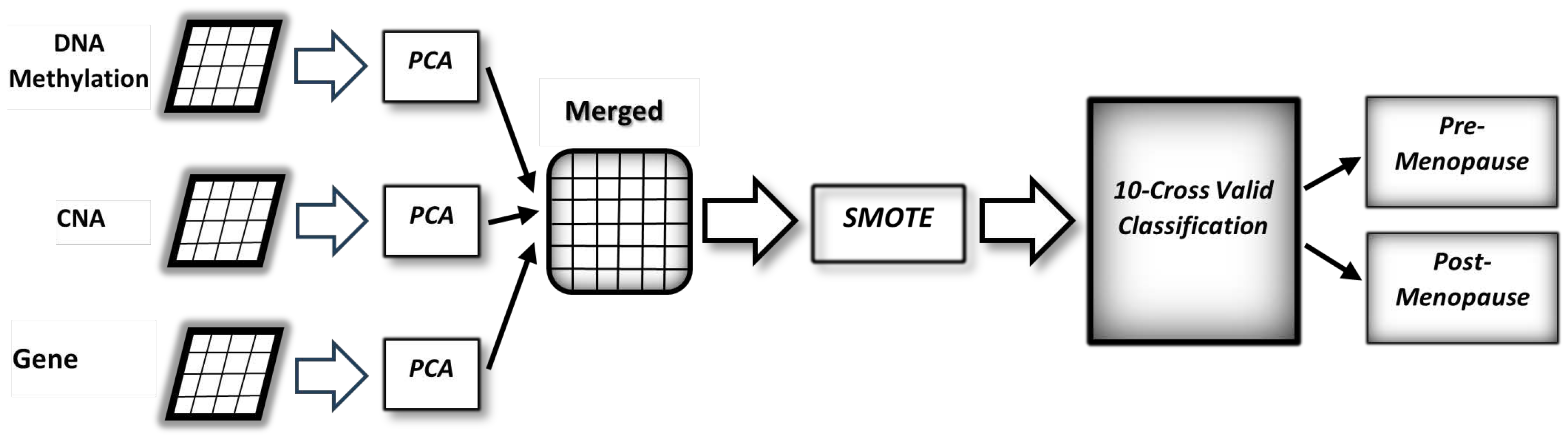
The various types of data and the proposed method are depicted in Figure 1. It starts by converting data to lower dimensions, then merging the converted data, and finally building a classification model to predict the status of menopause among breast cancer patients.

4. Materials

The publicly available TCGA Breast Invasive Carcinoma (BRCA) dataset was employed to investigate menopausal states [17]. It encompasses three distinct omics subdatasets: gene expression, DNA methylation, and copy number alteration (CNA). Only the samples with clear premenopause and postmenopause status were selected, and we neglected the intermediate samples. Out of 818 samples, a refinement process focusing only on samples with recorded data across all three omics reduced the total number of samples to 344. Among these, 89 samples were identified as premenopausal individuals, while the remaining 255 samples were postmenopausal individuals at the time of diagnosis. Each omic subdataset contains thousands of features. The dataset can be downloaded from https://www.cbioportal.org/study/summary?id=brca_tcga_pub2015 (accessed on 12 December 2023).

5. Preprocessing

Initially, gene expression features were filtered to exclude those with less than 0.2% variance, thereby resulting in a reduction in the count of gene expression features from approximately 39,000 to 16,000. Subsequently, normalization was applied to all three omics datasets using z-score normalization, while genes not following the Human Genome Organization (HUGO) format were removed. The final stage involved the identification of significantly mutated genes using the MutsigCV algorithm [18], which selects the genes with p values < 0.05 to be significantly mutated in breast cancer and calculates false discovery rates (FDRs). The input of MutsigCV is the mutated genes file supplied by the dataset. Genes exhibiting FDRs < 0.1 were recognized as significantly mutated, thereby leading to the selection of 14 mutated genes from the MutsigCV output for inclusion in this study.

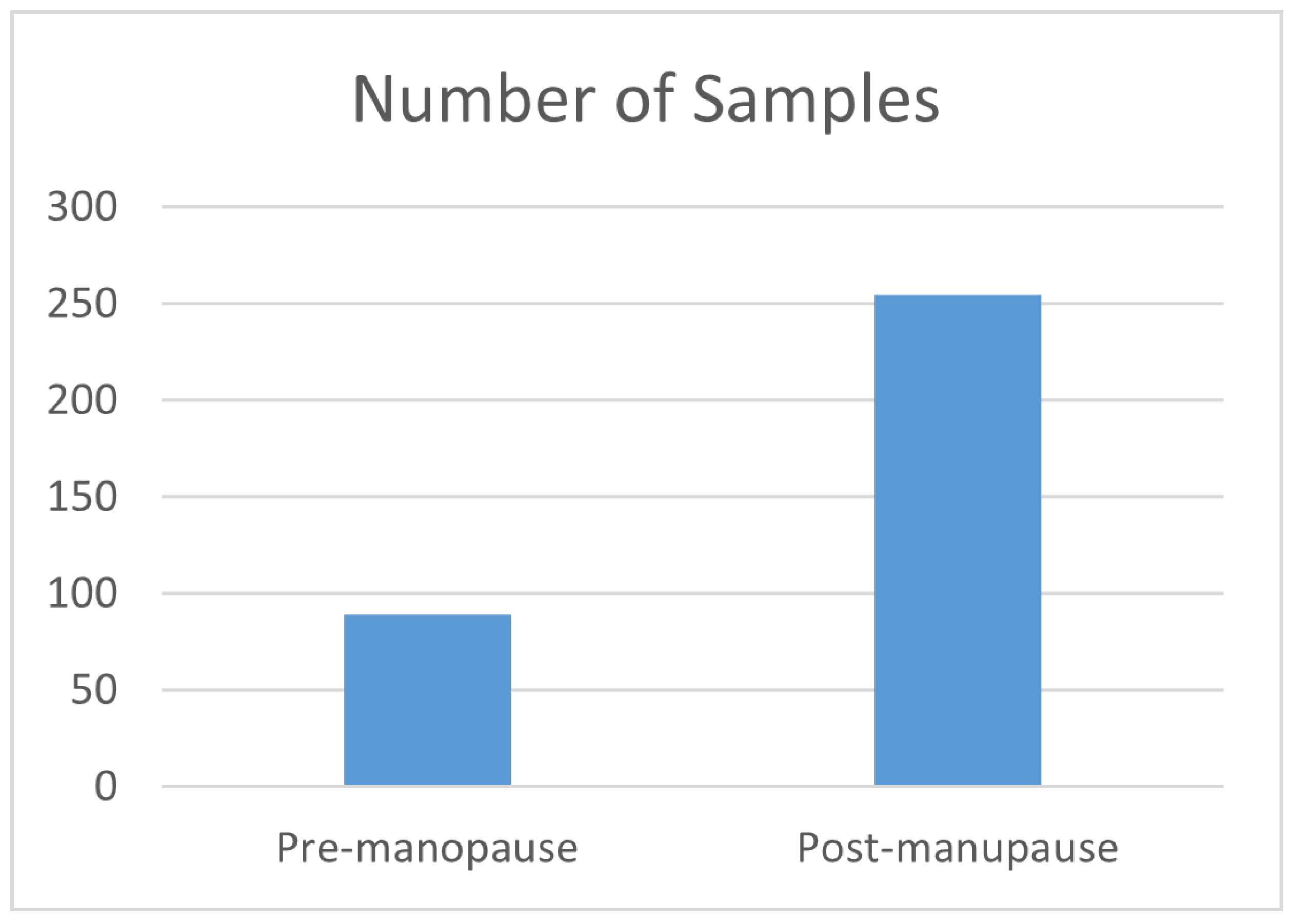
Figure 2 depicts the distribution of samples in premenopause and postmenopause classes, thereby showing that the dataset’s classes are imbalanced and suggesting the need to balance the data by up-sampling the minority class.

6. SMOTE

SMOTE is an up-sampling method for datasets with imbalanced classes. This technique generates new samples within the distribution of the minority class. SMOTE extracts feature vectors connecting existing samples and introducing synthetic samples along these connecting lines. The placement of each new synthetic sample on the connecting line is determined by calculating the distance between the two adjacent samples and then multiplying this distance by a randomly selected value between 0 and 1. This process effectively expands the representation of the minority class in the dataset by creating new synthetic instances that retain the characteristics of the original class while introducing controlled variation through the random factor [19].

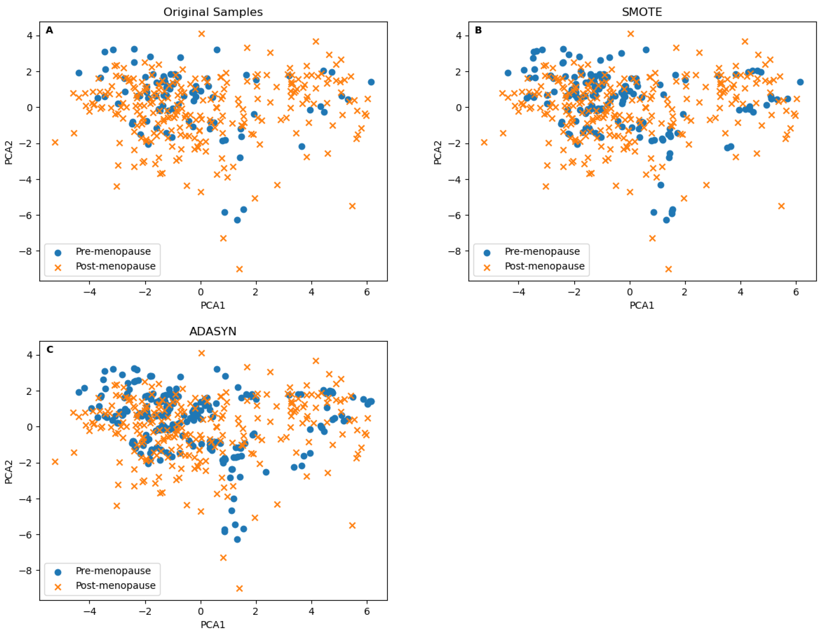
Before adopting SMOTE, we compared its resulting samples to the one generated by Adaptive Synthetic Sampling (ADASYN), which introduces adaptability based on local data density to focus more on difficult-to-classify instances [20]. ADASYN produced more samples in the less-dense area of the minor class, as seen in Figure 3C, compared to the SMOTE results in Figure 3B. It is hard to justify the validity of ADASYN samples in the class’s border area, mainly since some synthetically borderline samples were generated from a small number of samples, as seen in the original data samples in Figure 3A. SMOTE was able to generate samples in dense areas. This means that the newly generated samples were within a smaller distance of the original ones to justify the validity of the generated samples in clinical prediction and diagnostics applications. To validate the synthetic samples generated by both methods, we performed a Kolmogorov–Smirnov test for PCA1 and PCA2. The test was performed on the SMOTE synthetic samples versus the minor class’s samples from the original samples, and the same test was performed for the ADASYN synthetic samples. The p values of the first test were [PCA1 = 0.9999, PCA2 = 0.9999] and [PCA1 = 0.9895, PCA2 = 0.9539] for the second. Although both results are insignificant, they still show that the SMOTE synthetic samples are more strongly tied to the minor class than the ADASYN ones.

7. Principle Component Analysis

The model applies PCA to individual omic datasets to reduce complexities, remove noise, and identify shared patterns. Subsequently, these transformed PCA components from different omic datasets can be merged, thereby providing a more harmonized representation that encompasses the critical features across various omic layers [21]. This merged representation can then serve as a more robust foundation for constructing a prediction model, thereby ensuring improved interpretability, reduced overfitting, and enhanced generalization. The combined utilization of PCA and omic data integration thus equips us with a powerful means to derive meaningful insights and make accurate predictions in complex biological contexts [22]. The first step of PCA is to compute the covariance matrix C of the centred data Z. The covariance between two variables X_i and X_j is given by the following:

$$Cov(X_{\mathrm{i}},Y_{\mathrm{i}})=((Z_{\mathrm{i}}-mean\left(Z_{\mathrm{i}}\right))\times (Z_{\mathrm{j}}-mean\left(Z_{\mathrm{j}}\right)))/(n-1)$$

(1)

Therein, we then have the following:

• n is the number of data points.

The next step in is the number of data points in the matrix. Then, the model sorts the eigenvalues in decreasing order and chooses the top-k eigenvectors (principal components) corresponding to the largest eigenvalues. The last step is to project the centered data Z onto the new basis formed by the selected principal components. The covariance covered in the PCA was 0.95, and the transformed data Y is obtained by the following:

$$Y=Z\times V$$

(2)

Therein, we then have the following:

• V is the matrix containing the selected eigenvectors as columns.

8. Classification Models

The model combines the reduced data set from all omics into one data set labelled with 0 for premenopause samples and 1 for postmenopause samples. Three standard machine learning classifiers were applied to compare and select the proper method works on the reduced representation of various types of omic data, including Naïve Bayes, Random Forest, and the Support Vector Machine (SVM) with a Gaussian kernel.

9. Naïve Bayes Classifier

The Naïve Bayes classifier is a fundamental implementation of the Bayesian classifier. Despite its simplistic assumptions, such as feature independence given the class, Naïve Bayes often demonstrates impressive performance across various tasks. Given a dataset with features X = x₁, x₂, …, x_m and a set of classes C = c₁, c₂, …, c_m, the Naïve Bayes classifier computes the posterior probability of each class given the features using Bayes’ theorem:

$$P(c_{\mathrm{i}}\mid x_1,x_2,\dots ,x_{\mathrm{m}}\prod _{j=1}^{n}P\left(x_{\mathrm{j}}\right|c_{\mathrm{i}}))$$

(3)

Therein, we have the following:

• $P\left(c_{\mathrm{i}}\right)$ is the prior probability of class $c_{\mathrm{i}}$.
• $P(x_{\mathrm{j}}\mid c\mathrm{i})$ is the likelihood of feature $x_{\mathrm{j}}$ given class $c_i$ [23].

Due to its computational simplicity and ability to handle high-dimensional data, Naïve Bayes remains a popular choice for general classification, especially where efficiency and interpretability are crucial [24].

10. Random Forest Classifier

The Random Forest classifier stands out as a prominent ensemble learning method that has gained substantial attention in various machine learning applications. By aggregating the predictions of multiple decision trees, this approach provides enhanced accuracy, robustness, and flexibility. The prediction process of a Random Forest classifier can be represented as follows.

Given an ensemble to T decision trees T₁, T₂, …, T_T, each tree predicts the class label cT_i for an instance x. The final predicted class label C for x is determined through majority voting:

$$C=argma{x}_{\mathrm{i}}\sum _{t=1}^T\delta (c_{\mathrm{i}},T_{\mathrm{t}}\left(x\right))$$

(4)

Therein, we have the following:

• T is the total number of decision trees in the ensemble.
• $T_{\mathrm{x}}\left(x\right)$ is the class label predicated by $T_{\mathrm{t}}$ for instance x.
• $\delta (c_{\mathrm{i}},T_{\mathrm{t}}(x\left)\right)$ is the Kronecker delta function that equals 1 if $c_{\mathrm{i}}=T_{\mathrm{t}}\left(x\right)$ and 0 otherwise [25].

11. Support Vector Machine

The SVM is a classifier that finds a rule that can separate groups of datasets for classification and regression tasks [26]. In complex and high-dimensional datasets, one of SVM’s distinctive features is the ability to leverage kernel functions to handle nonlinear classification tasks. This work uses the Gaussian Radial Basis Function (RBF) kernel to find the hyperplane that separates the two classes. The primary objective of the SVM is to achieve maximum margin classification. The margin is the distance between the hyperplane and the nearest support vector of either class [27]. By incorporating the Gaussian kernel, the hyperplane formulation becomes the following:

$$f\left(x\right)=\sum _{i=1}^n{\alpha }_{\mathrm{i}}{y}_{\mathrm{i}}K(x,x_{\mathrm{i}})+b$$

(5)

Therein, we have the following:

• $f\left(x\right)$ is the decision function.
• $\alpha$_i are the LaGrange multipliers corresponding to support vectors.
• $x_{\mathrm{i}}$ is the class label of the ith instance.
• $K(x,x_{\mathrm{i}})$ is the RBF kernel function measuring similarity between input vectors x and $x_i$. It is the Gaussian kernel function.
• b is the bias term.

The $K(x,x_i)$ kernel function is expressed as the following equation:

$$K(x,x_i)=exp\left(-\gamma ·\Vert x-x_i{\Vert }^2\right)$$

(6)

Therein, we have the following:

• exp is the exponential function.
• $\gamma$ is the negative gamma parameter controlling the shape of the decision boundary.
• $\left(\Vert x-x_i{\Vert }^2\right)$ is the squared Euclidean distance between input vectors x and $x_i$, thereby measuring their closeness in the input space.

12. Results and Experiments

The three classification models were applied to the data set based on 10-fold crossvalidation. The following performance measurements for supervised learning classification methods were used to look at the performance from different perspectives including:

$$Precision={\displaystyle \frac{TP}{TP+FP}}$$

(7)

$$Recall={\displaystyle \frac{TP}{TP+FN}}$$

(8)

Therein, we have the following:

• $TP$ is true positive.
• $FP$ is false positive.
• $FN$ is false negative.

$$F-measure=2\times {\displaystyle \frac{P\times R}{P+R}}$$

(9)

Therein, we have the following:

• P is precision.
• R is recall.

$$AUCROC={\int }_0^{1}TPR\left(FPR\right).dFPR$$

(10)

Therein, we have the following:

• $TPR$ is the true positive rate and is used as a function.
• $FPR$ is the false positive rate.

$$Accuracy={\displaystyle \frac{TP+TN}{N}}$$

(11)

where:

• $TN$ is true negative.
• N is the number of all samples.

The hyperparameters of the SVM-RBF classifier were set to have $\gamma$ equal to 0.02 and the cost of determining the margins to remain at the default, that is, at one. For the Random Forest, the number of trees was set to be 1000, and the number of features at each split equaled $lo{g}_2\left(m\right)$, where m is the number of features. The Naive Bayes was run using the default parameters in the sickit-learn library.

Table 1. The performance measurements of the three classification models on the breast cancer multiomics dataset.

Model/ Measure	Precision	Recall	F Measure	AUCROC	Accuracy	Confusion Matrix
Naïve Bayes	0.7614	0.788	0.775	0.816	72.98%	TP = 201, FN = 54, TN = 115, FP = 63
Random Forest	0.914	0.886	0.90	0.962	88.45%	TP = 226, FN = 29, TN = 157, FP = 21
SVM-RBF	0.919	0.894	0.907	0.886	89.14%	TP = 228, FN = 27, TN = 158, FP = 20

shows the scores of the performance measurements for the Naïve Bayes, Random Forest, and SVM-RBF classifiers. Random Forest outperformed the other two classifiers with an area under the curve of the “Receiver Operating Characteristic” (AUCROC) of 0.962 compared to 0.886 for the second, which was SVM-RBF. SVM-RBF outperformed the other two classifiers with an accuracy of 89.53% compared to the runner-up Random Forest with an accuracy of 88.54%. Naïve Bayes performed poorly in all measures compared to the other two classifiers.

12.1. Gene Expression Feature Importance Validation

To find the contribution of each class in the classification model, we employed Explainable Artificial Intelligence (AI) techniques, specifically the Shapley Additive Explanations (SHAP) method [28], to elucidate the significance of gene expression features in distinguishing between premenopause and postmenopause breast cancer samples using the XGBoost regressor [29]. This approach allowed us to interpret the complex decision-making process of the XGBoost model and to understand the impact of individual gene expressions on the classification outcome. SHAP values provide a comprehensive understanding of the contribution of each gene expression feature to the model’s predictions, thereby aiding in the identification of key factors influencing the classification of menopausal status in breast cancer samples. We aimed to extract meaningful insights into the biological mechanisms underlying the menopausal distinctions in breast cancer.

The SHAP values ${\varphi }_i\left(f\right)$ for feature i are calculated using the following formula:

$${\varphi }_i\left(f\right)=\sum _{S\subseteq N\setminus \left\{i\right\}}\frac{\left(\right|S|-1)!·\left(\right|N|-|S\left|\right)!}{\left|N\right|!}[f(S\cup \left\{i\right\})-f\left(S\right)]$$

(12)

Therein, we have the following:

• N represents the set of all features.
• S is a subset of features excluding feature i.
• $\left|S\right|$ denotes the cardinality of set S.
• $f\left(S\right)$ denotes the model’s prediction with the features in subset S.

These SHAP values provide a quantitative measure of the impact of each gene expression feature on the output. The XGBoost prediction for a sample i is given by ${\widehat{y}}_i=\psi \left({\mathbf{x}}_i\right)$, where $\psi$ is the sum of predictions from individual decision trees ${\psi }_k$ in the ensemble. Mathematically, this is represented as

$${\widehat{y}}_i=\sum _{k=1}^K{\psi }_k\left({\mathbf{x}}_i\right),{\psi }_k\in \mathcal{Y}$$

(13)

Therein, we have the following:

• K is the total number of trees.
• ${\psi }_k$ represents an individual decision tree from the set of all possible decision trees denoted by $\mathcal{Y}$.

The final prediction combines predictions from all trees, thereby providing a powerful and flexible model for classification tasks.

12.2. Kaplan-Meier

The Kaplan–Meier estimator is a nonparametric method that is widely used for estimating the survival function from time-to-event data. The survival function, denoted as $S\left(t\right)$, represents the probability that the death event occurs after a specified time t. The estimator is calculated based on the observed survival times in a given dataset. Let n be the number of individuals in the sample, d be the number of observed events, and $t_1,t_2,\dots t_i,t_j$ be the observed event times. The Kaplan–Meier estimator at time t is given by the following formula:

$$S\left(t\right)=\prod _{i=1}^j\left(1-\frac{d_i}{n_i}\right)$$

(14)

Therein, we have the following:

• j represents the distinct event times.
• $d_i$ is the number of events at time $t_i$.
• $n_i$ is the number of individuals at risk just before time $t_i$.

The product is taken over all event times $t_i$ less than or equal to t. This estimator allows us to visualize and analyze survival curves over time, thereby providing valuable insights into the probability of survival at different time points in a study [30].

12.3. Running Environment

We ran the model on Microsoft Azure cloud computing machine “Standard_F4s_v2” that is built on four cores, 8 GB RAM, and 32 GB storage. The coding environment was a Jupyter Notebook.

13. Discussion

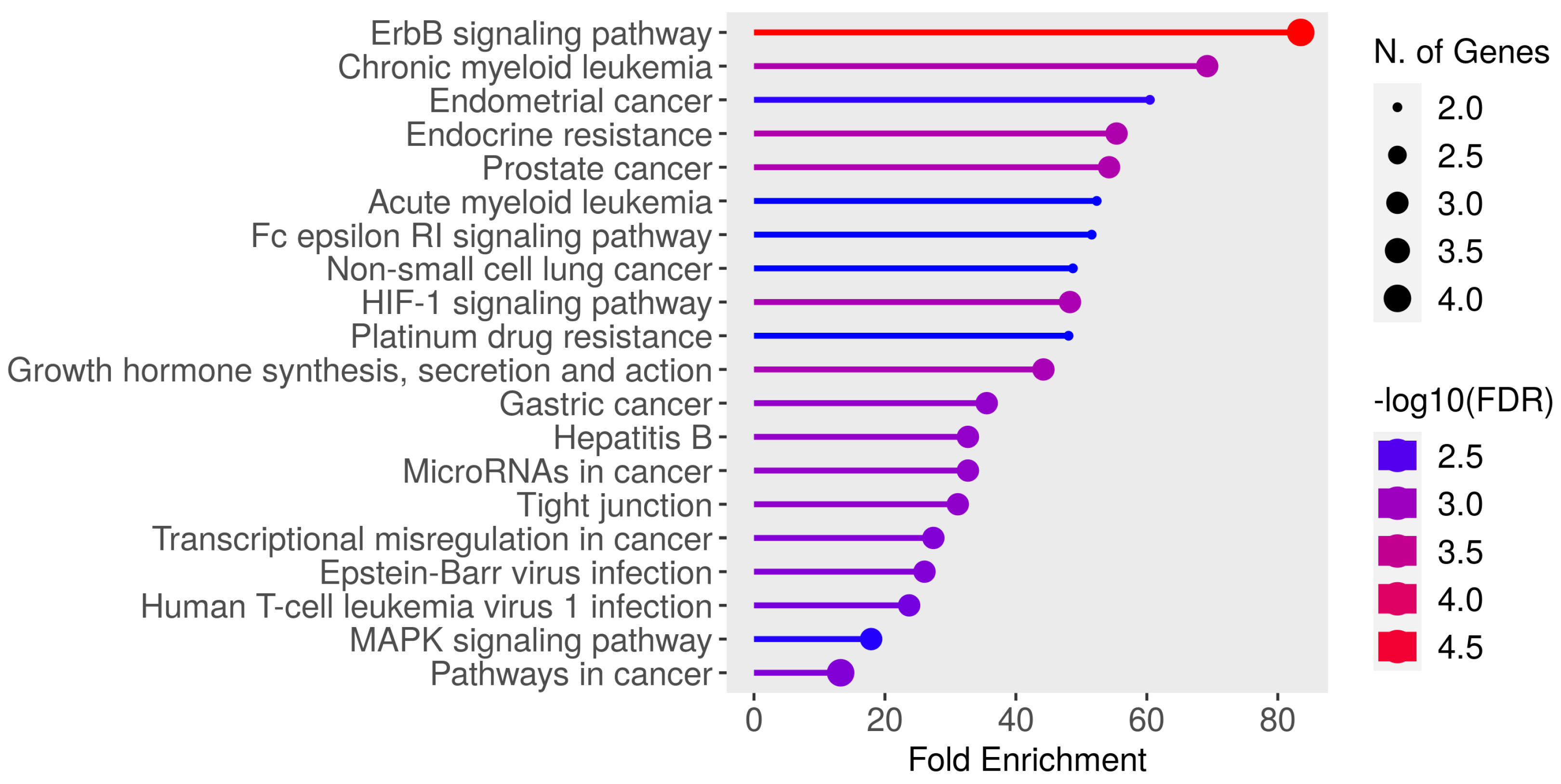
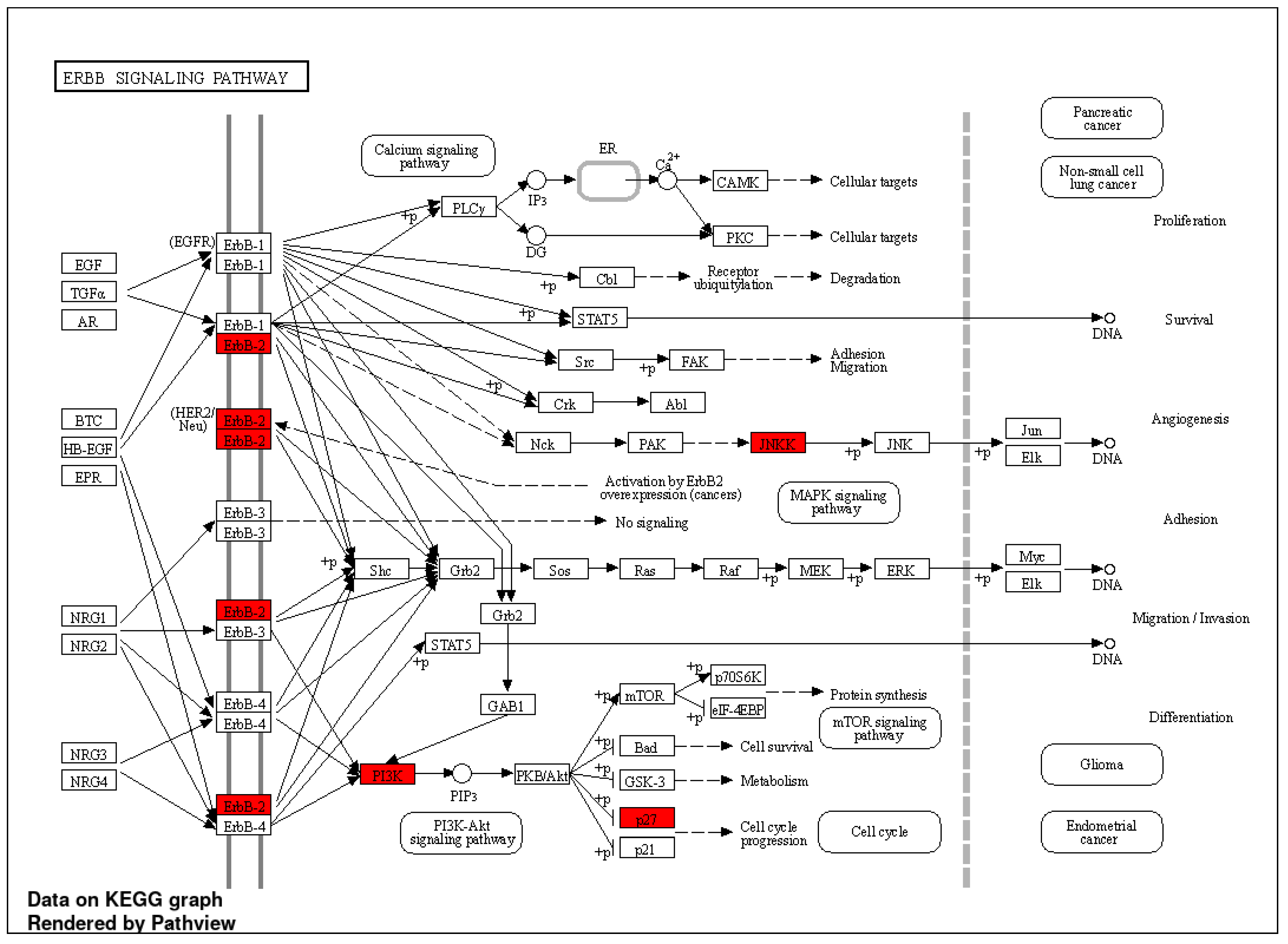
The selected genes showed a discriminative power in predicting the breast cancer menopause status. By running GO enrichment analysis using ShinyGO [31] on the selected genes, many of these genes were confirmed to be related to various types of cancer, as seen in Figure 4. It can be noticed in Figure 4 that the “ErbB signaling pathway” had the highest fold enrichment score. KEGG pathway [32] analysis was applied to the selected genes to visualize the ErbB signaling pathway as shown in Figure 5. Tian et al. reported the ErbB signaling pathway in association with the menopausal syndrome in their ontological analysis [33]. Pei et al. found a cardiorenal disease connection during postmenopause with ErbB signaling pathway genes [34], which sparked the idea of the survival analysis of the two cohorts in our work.

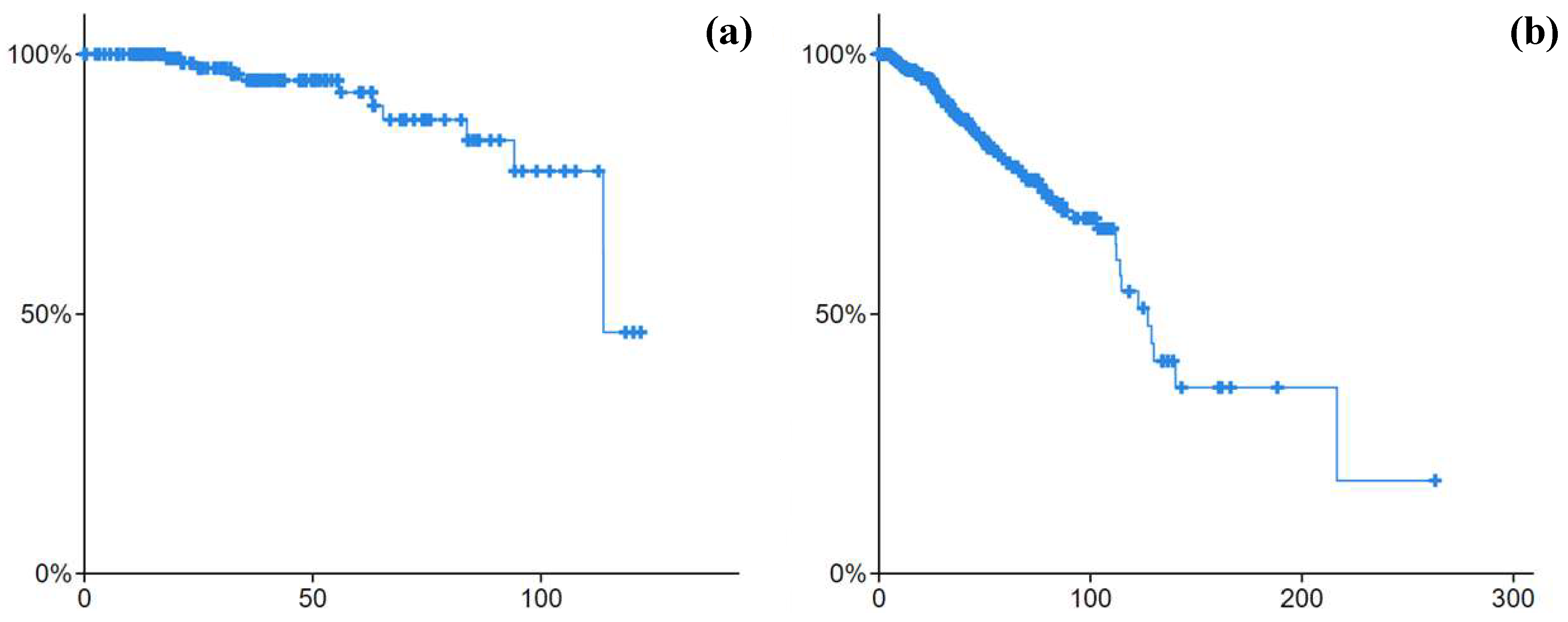
The Kaplan–Meier analysis for the patients in both cohorts with p value < 0.05 showed a different survivability chance for the patients between them. The survivability curve for the premenopause class (the one in Figure 6a) was higher than the postmenopause class (the one in Figure 6b). The identified omics biomarkers for the significantly different survival populations may indicate a signature for both classes.

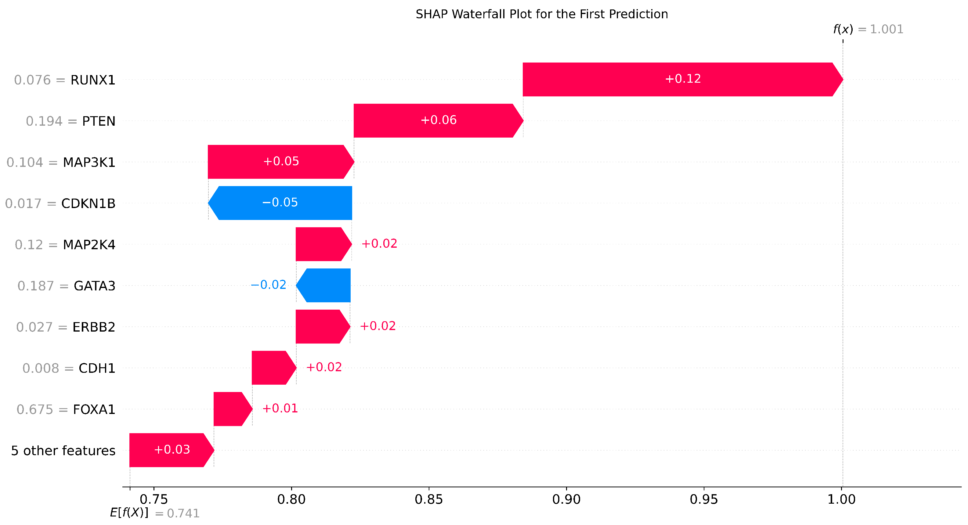
To show the importance of the gene expression values, we ran the SHAP model on XGBoost to determine the most discriminative genes. Figure 7 shows the feature importance based on how much the gene expression value impacted the classification model. The results suggest that RUNX1, PTEN, MAP3K1, and CDH1 significantly distinguished the two classes.

Riggio stated that RUNX1 acts as a tumour suppressor at the early stages of breast cancer, while it acts as a pro-oncogene at later stages of mammary tumourigenesis. The study discussed the involvement of RUNX family of transcription factors in various types of cancers and the changes that occur in the human breast of older women (particularly after menopause) [36]. While Zhang et al. reported no significant correlation between RUNX1 gene expression and menopause status, PTEN is still important for the tumorigenesis, development, and the prognosis of breast cancer [37].

Rebbeck et al. reported that the MAP3K1 gene confers its effects in HER2 tumors, which was shown to affect breast cancer susceptibility in African American women. It also interacts with hormone exposures in African American and European American women [38]. Postmenopausal women with a higher histological grade and PR- tumors exhibited a notably intensified methylation of the CDH1 promoter compared to cases with PR+ tumors [39].

In future research, expanding the proposed framework to include additional omics data types, including proteomics and metabolomics, can provide a more holistic understanding of the molecular landscape associated with the menopause status of breast cancer. PCA reduction may work well in integrating the quantifications of metabolites and merging the abundance measurements of proteomics, including spectral counts, normalized spectral abundance factor (NSAF), and extracted ion chromatogram (XIC) peak area into the model. Investigating the longitudinal aspects of menopausal transitions and their dynamic influence on the identified biomarkers may offer valuable insights into the temporal relationships between genetic and epigenetic alterations and breast cancer development. Integrating clinical variables, such as hormone receptor status and treatment history, into the analysis could enhance the clinical relevance of the identified biomarkers, thereby providing a more comprehensive picture of their associations with menopausal status and breast cancer outcomes. The hormone receptor status can be investigated by studying the resulting folded enrichment pathways in Figure 4, and the treatment history can be added as a second label for the menopausal status class. The availability of comprehensive multiomics datasets, especially in the context of menopausal breast cancer, is currently limited. However, with the advancement of next-generation sequencing and other omics approaches, more datasets could be available for better validation.

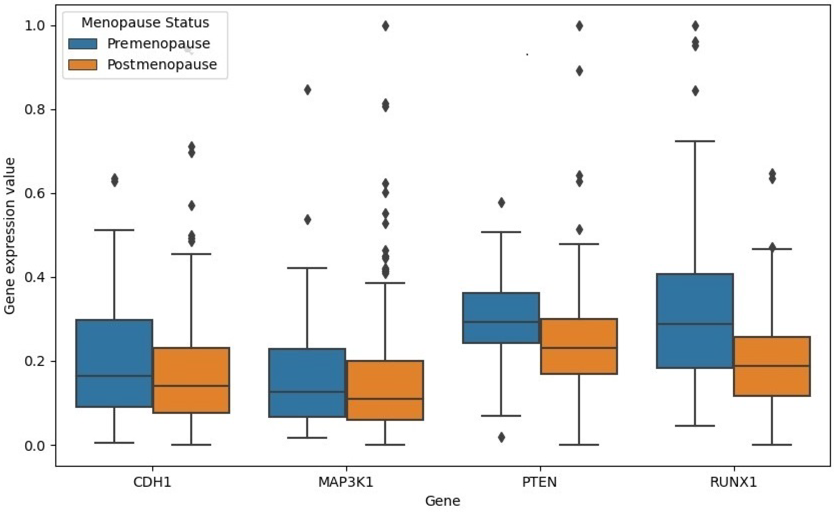
Figure 8 shows the boxplots for the gene expressions of the four genes in both classes. The four genes showed lower expression values in the postmenopause cohort of samples.

$8\times {10}^{-3}$ As seen in Figure 8, CDH1, PTEN, and RUNX1 significantly down-regulated in the postmenopause class compared to the premenopause class with p values < 0.05. The difference between gene expression values for MAP3K1 is not significant. Unlike the remaining three genes, the RUNX1 gene expression values had no outliers in the premenopause class compared to the postmenopause class.

To study the relationships between the resulting genes in each omic, Pearson correlation analysis for the genes in each omic has been included in the Supplementary Materials in Figures S1–S3. The crosstalk between the genes in the three omics is a limitation of this work and can be analyzed in a more detailed network analysis in future work.

14. Conclusions

This work proposed a pipeline to integrate multiomics data to classify the menopause status in female breast cancer. The aim of the study was to identify multiomics biomarkers for premenopause and postmenopause to understand how this physical and emotional change is reflected in the molecular base in breast cancer tissue. The dataset contains gene expression, CNA, and DNA methylation data that are processed and merged into a classification model based on 10 crossvalidations. SVM-RBF, Random Forest, and Naïve Bayes were tested in the merged data.

Recognizing the imbalance in the distribution of samples between premenopause and postmenopause classes, we addressed this issue using the Synthetic Minority Over-sampling Technique (SMOTE). This up-sampling method generated synthetic samples within the minority class, thereby providing a more balanced dataset for subsequent analyses.

The Random Forest exhibited the highest performance with an AUCROC of 0.962, while the SVM-RBF demonstrated superior accuracy, thereby achieving 89.53%. Pathway analysis on the selected genes revealed an association between those genes and some cancer pathways; one of them is the “ErbB signaling pathway”, which was reported to be associated with menopausal syndrome and cardiorenal disease. The survival analysis for both classes, premenopause and postmenopause in breast cancer, showed a significant difference in the survival rate between them, which makes them two distinct populations, with each having its own characteristics. Explainable AI Shapley based on XGBoost showed that RUNX1, PTEN, MAP3K1, and CDH1 had the highest impact in distinguishing the two classes. The literature confirmed the associations between each one of them with breast cancer in general and menopause status.

The source code is available on the following GitHub repository: https://github.com/dtabed/PCAOMICS (accessed on 12 December 2023).

References

- Steve Becker, T. A historic and scientific review of breast cancer: The next global healthcare challenge. Int. J. Gynecol. Obstet. 2015, 131, S36–S39. [Google Scholar]
- Sung, H.; Ferlay, J.; Siegel, R.L.; Laversanne, M.; Soerjomataram, I.; Jemal, A.; Bray, F. Global cancer statistics 2020: Globocan estimates of incidence and mortality worldwide for 36 cancers in 185 countries. CA Cancer J. Clin. 2021, 71, 209–249. [Google Scholar] [CrossRef] [PubMed]
- Yardley, D.A.; Ismail-Khan, R.R.; Melichar, B.; Lichinitser, M.; Munster, P.N.; Klein, P.M.; Cruickshank, S.; Miller, K.D.; Lee, M.J.; Trepel, J.B. Randomized phase ii, double-blind, placebo-controlled study of exemestane with or without entinostat in postmenopausal women with locally recurrent or metastatic estrogen receptor-positive breast cancer progressing on treatment with a nonsteroidal aromatase inhibitor. J. Clin. Oncol. 2013, 31, 2128. [Google Scholar] [PubMed]
- Yardley, D.A.; Noguchi, S.; Pritchard, K.I.; Burris, H.A.; Baselga, J.; Gnant, M.; Hortobagyi, G.N.; Campone, M.; Pistilli, B.; Piccart, M.; et al. Everolimus plus exemestane in postmenopausal patients with HR(+) breast cancer: BOLERO-2 final progression-free survival analysis. Adv. Ther. 2013, 30, 870–884. [Google Scholar] [CrossRef]
- Tromberg, B.J.; Cerussi, A.; Shah, N.; Compton, M.; Durkin, A.; Hsiang, D.; Butler, J.; Mehta, R. Imaging in breast cancer: Diffuse optics in breast cancer: Detecting tumors in pre-menopausal women and monitoring neoadjuvant chemotherapy. Breast Cancer Res. 2005, 7, 1–7. [Google Scholar] [CrossRef] [PubMed]
- Vincent, A. Management of menopause in women with breast cancer. Climacteric 2015, 18, 690–701. [Google Scholar] [CrossRef] [PubMed]
- O’neill, P.A.; Davies, M.P.A.; Shaaban, A.M.; Innes, H.; Torevell, A.; Sibson, D.R.; Foster, C. Wild-type oestrogen receptor beta (erβ1) mrna and protein expression in tamoxifen-treated post-menopausal breast cancers. Br. J. Cancer 2004, 91, 1694–1702. [Google Scholar] [CrossRef]
- Crujeiras, A.B.; Diaz-Lagares, A.; Stefansson, O.A.; Macias-Gonzalez, M.; Sandoval, J.; Cueva, J.; Lopez-Lopez, R.; Moran, S.; Jonasson, J.G.; Tryggvadottir, L.; et al. Obesity and menopause modify the epigenomic profile of breast cancer. Endocr. Relat. Cancer 2017, 24, 351–363. [Google Scholar] [CrossRef]
- Zhou, L.; Rueda, M.; Alkhateeb, A. Classification of breast cancer Nottingham prognostic index using high-dimensional embedding and residual neural network. Cancers 2008, 14, 934. [Google Scholar] [CrossRef]
- Froehlich, H.; Patjoshi, S.; Yeghiazaryan, K.; Kehrer, C.; Kuhn, W.; Golubnitschaja, O.T. The title of the cited article. EPMA J. 2018, 9, 175–186. [Google Scholar]
- Egelston, C.A.; Guo, W.; Tan, J.; Avalos, C.; Simons, D.L.; Lim, M.H.; Huang, Y.J.; Nelson, M.S.; Chowdhury, A.; Schmolze, D.B.; et al. Tumor-infiltrating exhausted cd8+ t cells dictate reduced survival in premenopausal estrogen receptor—Positive breast cancer. JCI Insight 2022, 7, e153963. [Google Scholar] [CrossRef] [PubMed]
- Assi, N.; Moskal, A.; Slimani, N.; Viallon, V.; Chajes, V.; Freisling, H.; Monni, S.; Knueppel, S.; Foerster, J.; Weiderpass, E.; et al. A treelet transform analysis to relate nutrient patterns to the risk of hormonal receptor-defined breast cancer in the european prospective investigation into cancer and nutrition (epic). Public Health Nutr. 2016, 19, 242–254. [Google Scholar] [CrossRef] [PubMed]
- Qattous, H.; Azzeh, M.; Ibrahim, R.; AbedalGhafer, I.; Al Sorkhy, M.; Alkhateeb, A. Pacmap-embedded convolutional neural network for multi-omics data integration. Heliyon 2024, 10, e23195. [Google Scholar] [CrossRef]
- Van der Maaten, L.; Hinton, G. Visualizing data using t-sne. J. Mach. Learn. Res. 2008, 9, 2579–2605. [Google Scholar]
- Wang, Y.; Huang, H.; Rudin, C.; Shaposhnik, Y. Understanding how dimension reduction tools work: An empirical approach to deciphering t-sne, umap, trimap, and pacmap for data visualization. J. Mach. Learn. Res. 2021, 22, 1–73. [Google Scholar]
- Argelaguet, R.; Velten, B.; Arnol, D.; Dietrich, S.; Zenz, T.; Marioni, J.C.; Buettner, F.; Huber, W.; Stegle, O. Multi-omics factor analysis—A framework for unsupervised integration of multi-omics data sets. Mol. Syst. Biol. 2018, 14, e8124. [Google Scholar] [CrossRef] [PubMed]
- Ciriello, G.; Gatza, M.L.; Beck, A.H.; Wilkerson, M.D.; Rhie, S.K.; Pastore, A.; Zhang, H.; McLellan, M.; Yau, C.; Kandoth, C.; et al. Comprehensive molecular portraits of invasive lobular breast cancer. Cell 2015, 163, 506–519. [Google Scholar] [CrossRef] [PubMed]
- Lawrence, M.S.; Stojanov, P.; Polak, P.; Kryukov, G.V.; Cibulskis, K.; Sivachenko, A.; Carter, S.L.; Stewart, C.; Mermel, C.H.; Roberts, S.A.; et al. Mutational heterogeneity in cancer and the search for new cancer-associated genes. Nature 2013, 499, 214–218. [Google Scholar] [CrossRef]
- Chawla, N.V.; Bowyer, K.W.; Hall, L.O.; Kegelmeyer, W.P. SMOTE: Synthetic minority over-sampling technique. J. Artif. Intell. Res. 2022, 10, 142–149. [Google Scholar] [CrossRef]
- He, H.; Bai, Y.; Garcia, E.A.; Li, S. Adasyn: Adaptive synthetic sampling approach for imbalanced learning. In Proceedings of the 2008 IEEE International Joint Conference on Neural Networks (IEEE World Congress on Computational iIntelligence), Hong Kong, China, 1–8 June 2008; IEEE: Piscataway, NJ, USA, 2008; pp. 1322–1328. [Google Scholar]
- Wold, S.; Esbensen, K.; Geladi, P. Principal component analysis. Chemom. Intell. Lab. Syst. 2008, 2, 37–52. [Google Scholar] [CrossRef]
- Athieniti, E.; Spyrou, G.M. A guide to multi-omics data collection and integration for translational medicine. Comput. Struct. Biotechnol. J. 2023, 21, 134–149. [Google Scholar] [CrossRef] [PubMed]
- Lewis, D.D. Naive (bayes) at forty: The independence assumption in information retrieval. In Machine Learning: ECML-98; Nédellec, C., Rouveirol, C., Eds.; Springer: Berlin/Heidelberg, Germany, 1998; pp. 4–15. [Google Scholar]
- BAYES. An essay towards solving a problem in the doctrine of chances. Biometrika 1958, 45, 296–315. [Google Scholar] [CrossRef]
- Breiman, L. Random forests. Mach. Learn. 2001, 45, 5–32. [Google Scholar] [CrossRef]
- Cortes, C.; Vapnik, V. Support-vector networks. Mach. Learn. 1995, 20, 273–297. [Google Scholar] [CrossRef]
- Wang, J.; Chen, Q.; Chen, Y. RBF Kernel Based Support Vector Machine with Universal Approximation and Its Application. Int. Symp. Neural Netw. 2008, 10, 512–517. [Google Scholar]
- Shapley, L.S. Notes on the n-Person Game—II: The Value of an n-Person Game; RAND Corporation: Santa Monica, CA, USA, 1951. [Google Scholar]
- Chen, T.; Guestrin, C. Xgboost: A scalable tree boosting system. In Proceedings of the 22nd ACM Sigkdd International Conference on Knowledge Discovery and Data Mining, San Francisco, CA, USA, 13–17 August 2016; pp. 785–794. [Google Scholar]
- Kaplan, E.L.; Meier, P. Nonparametric estimation from incomplete observations. J. Am. Stat. Assoc. 1958, 53, 457–481. [Google Scholar] [CrossRef]
- Ge, S.X.; Jung, D.; Yao, R. ShinyGO: A graphical gene-set enrichment tool for animals and plants. Bioinformatics 2008, 36, 2628–2629. [Google Scholar] [CrossRef] [PubMed]
- Kanehisa, M.; Furumichi, M.; Sato, Y.; Ishiguro-Watanabe, M.; Tanabe, M. KEGG: Integrating viruses and cellular organisms. Nucleic Acids Res. 2008, 49, D545–D551. [Google Scholar] [CrossRef]
- Tian, M.; Yang, A.; Lu, Q.; Zhang, X.; Liu, G.; Liu, G. Study on the mechanism of baihe dihuang decoction in treating menopausal syndrome based on network pharmacology. Medicine 2023, 102, e33189. [Google Scholar] [CrossRef]
- Pei, J.; Harakalova, M.; den Ruijter, H.; Pasterkamp, G.; Duncker, D.J.; Verhaar, M.C.; Asselbergs, F.W.; Cheng, C. Cardiorenal disease connection during post-menopause: The protective role of estrogen in uremic toxins induced microvascular dysfunction. Int. J. Cardiol. 2017, 238, 22–30. [Google Scholar] [CrossRef]
- Luo, W.; Brouwer, C. Pathview: An R/Bioconductor package for pathway-based data integration and visualization. Bioinformatics 2013, 29, 1830–1831. [Google Scholar] [CrossRef] [PubMed]
- Riggio, A.I. The Role of Runx1 in Genetic Models of Breast Cancer. Ph.D. Thesis, University of Glasgow, Scotland, UK, 2017. [Google Scholar]
- Zhang, H.Y.; Liang, F.; Jia, Z.L.; Song, S.T.; Jiang, Z.F. Pten mutation, methylation and expression in breast cancer patients. Oncol. Lett. 2013, 6, 161–168. [Google Scholar] [CrossRef] [PubMed]
- Rebbeck, T.R.; DeMichele, A.; Tran, T.V.; Panossian, S.; Bunin, G.R.; Troxel, A.B.; Strom, B.L. Hormone-dependent effects of fgfr2 and map3k1 in breast cancer susceptibility in a population-based sample of post-menopausal african-american and european-american women. Carcinogenesis 2009, 30, 269–274. [Google Scholar] [CrossRef] [PubMed][Green Version]
- Sebova, K.; Zmetakova, I.; Bella, V.; Kajo, K.; Stankovicova, I.; Kajabova, V.; Krivulcik, T.; Lasabova, Z.; Tomka, M.; Galbavy, S.; et al. Rassf1a and cdh1 hypermethylation as potential epimarkers in breast cancer. Cancer Biomark. 2012, 10, 13–26. [Google Scholar] [CrossRef]