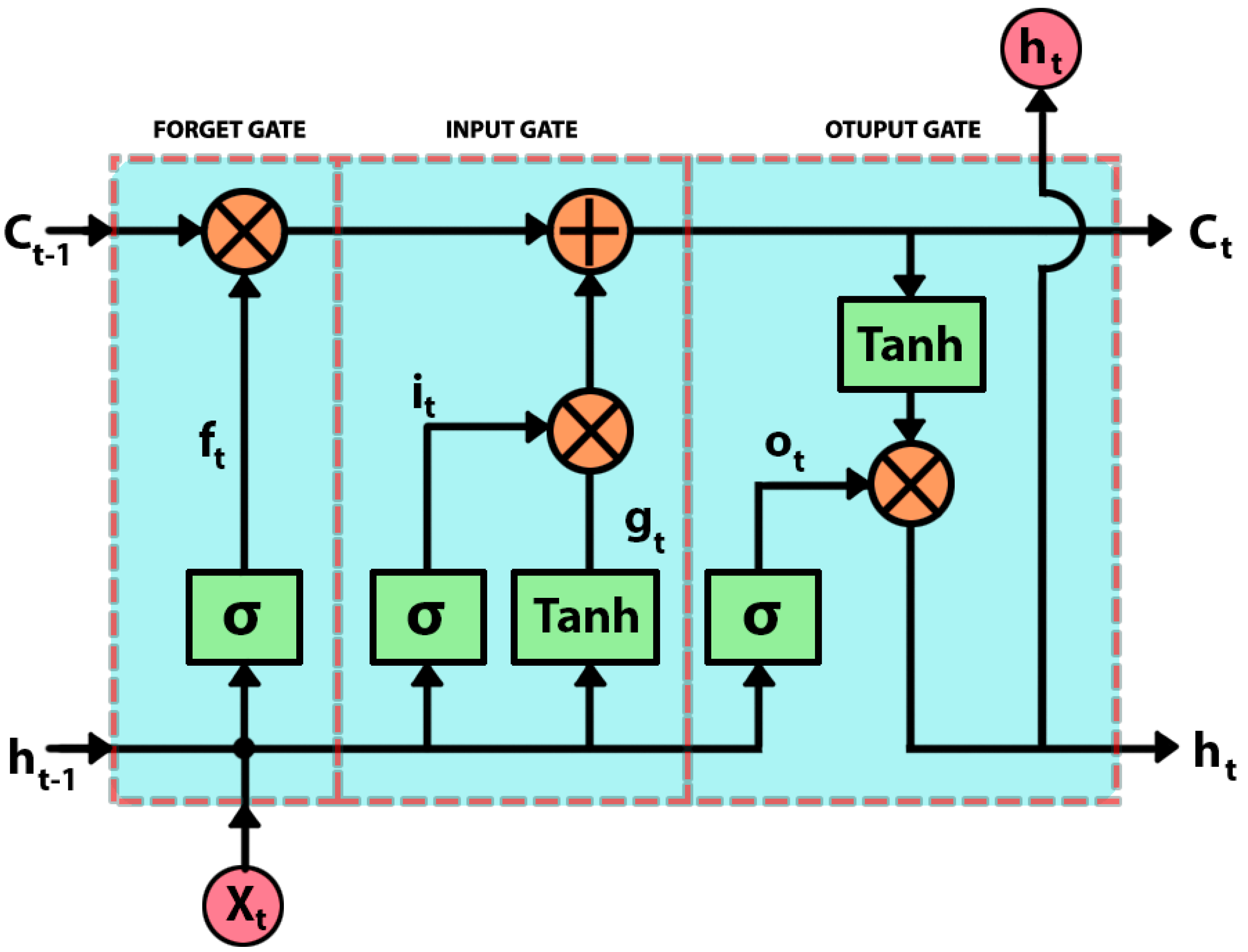
Figure 1.
LSTM neuron structure (Forget gate, Input gate, Output gate) stands for sigmoid function, the input data, and the current network output.
Figure 1.
LSTM neuron structure (Forget gate, Input gate, Output gate) stands for sigmoid function, the input data, and the current network output.
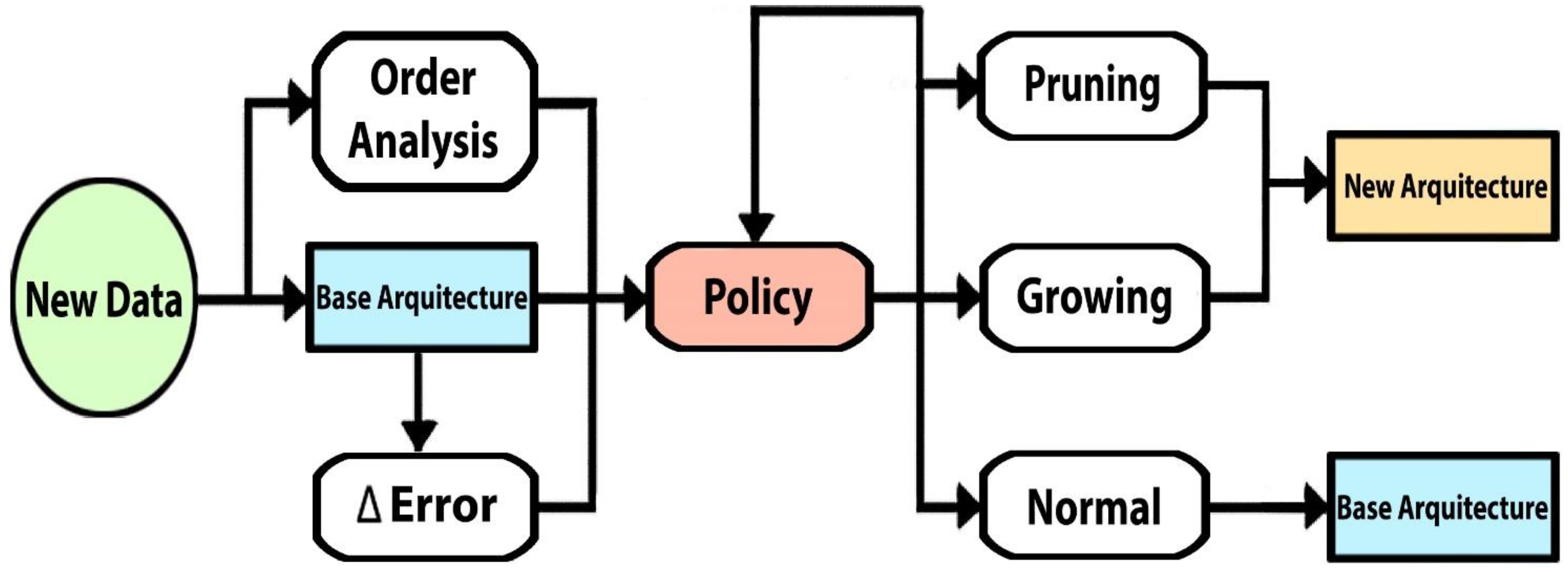
Figure 2.
Dynamic architecture algorithm for RNN flowchart.
Figure 2.
Dynamic architecture algorithm for RNN flowchart.
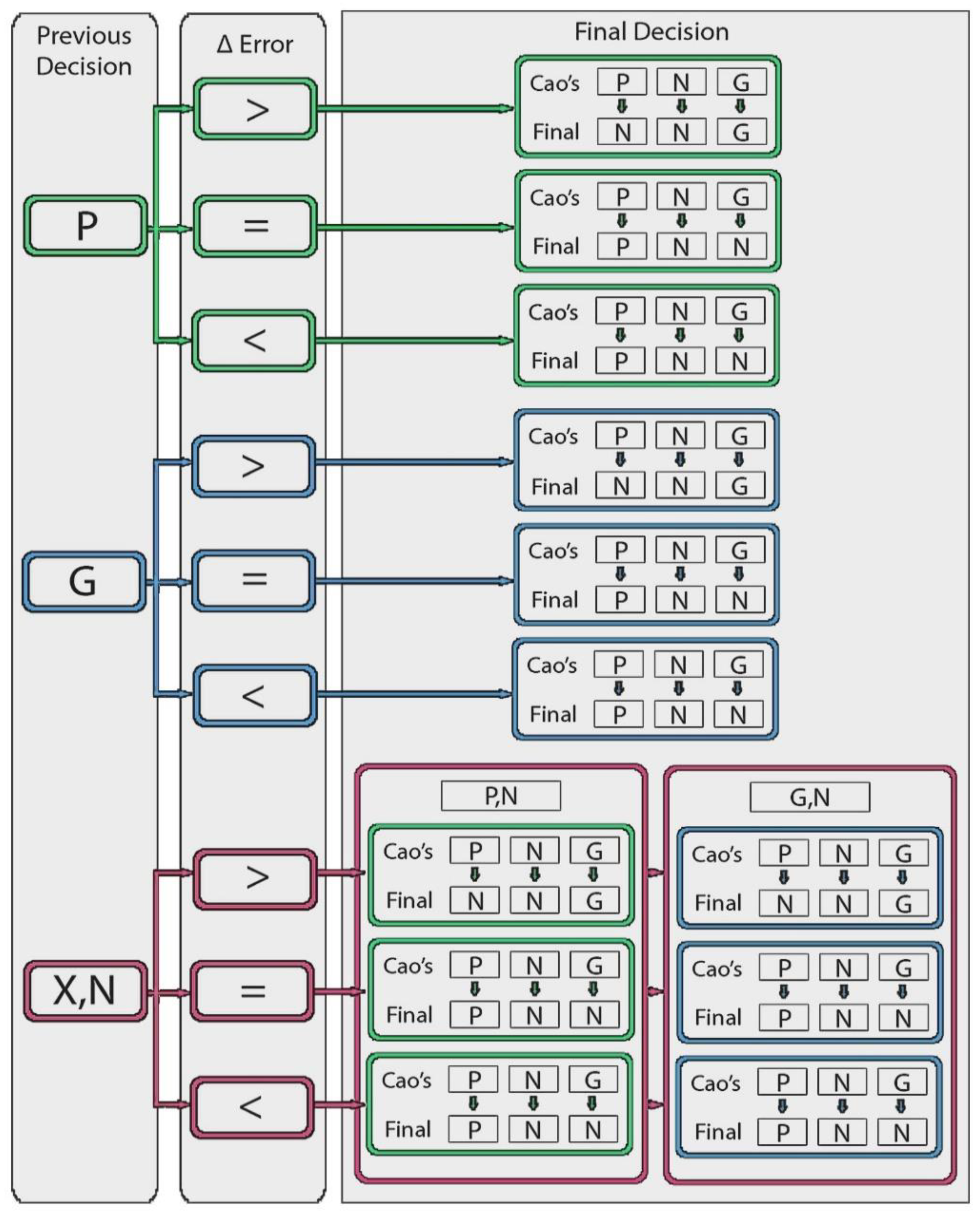
Figure 3.
Decision tree, [P = Pruning, G = Growing, N = Normal, X = Last decision different from N.
Figure 3.
Decision tree, [P = Pruning, G = Growing, N = Normal, X = Last decision different from N.
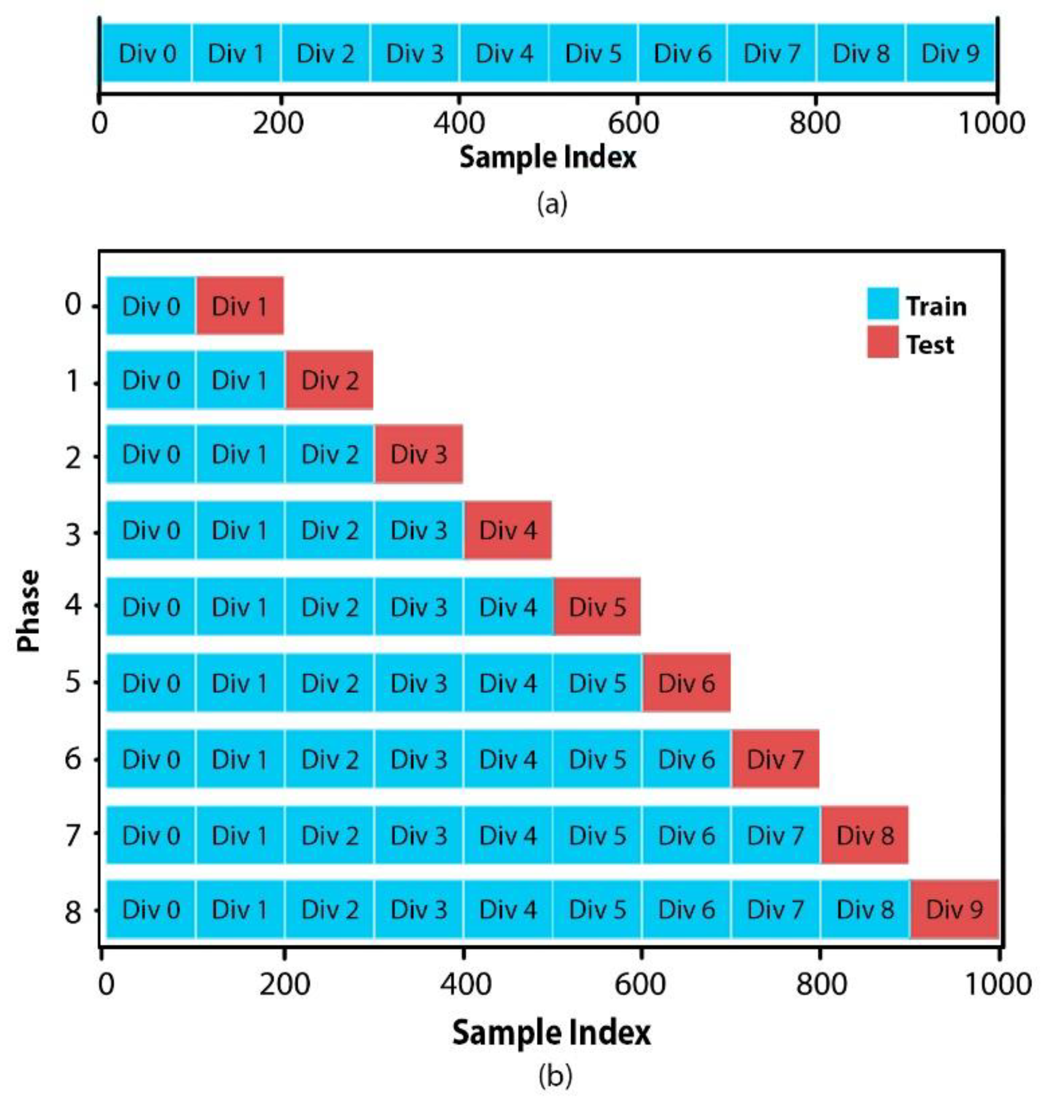
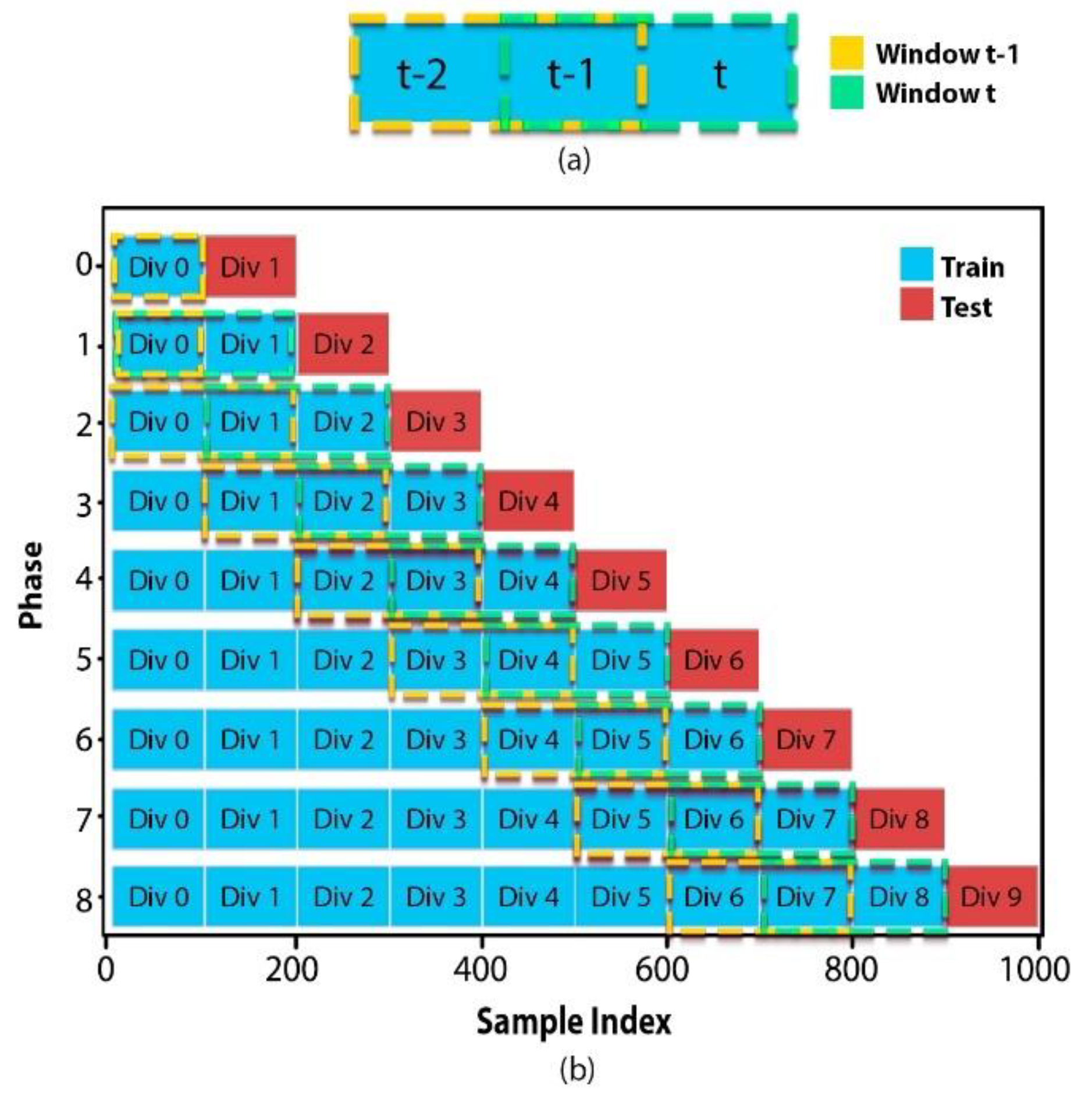
Figure 4.
Data distribution: (a) Data set divisions, (b) Train and Test subsets on each phase.
Figure 4.
Data distribution: (a) Data set divisions, (b) Train and Test subsets on each phase.
Figure 5.
Mobile window for order calculation: (a) Generation of windows, (b) Movement of windows on each phase.
Figure 5.
Mobile window for order calculation: (a) Generation of windows, (b) Movement of windows on each phase.
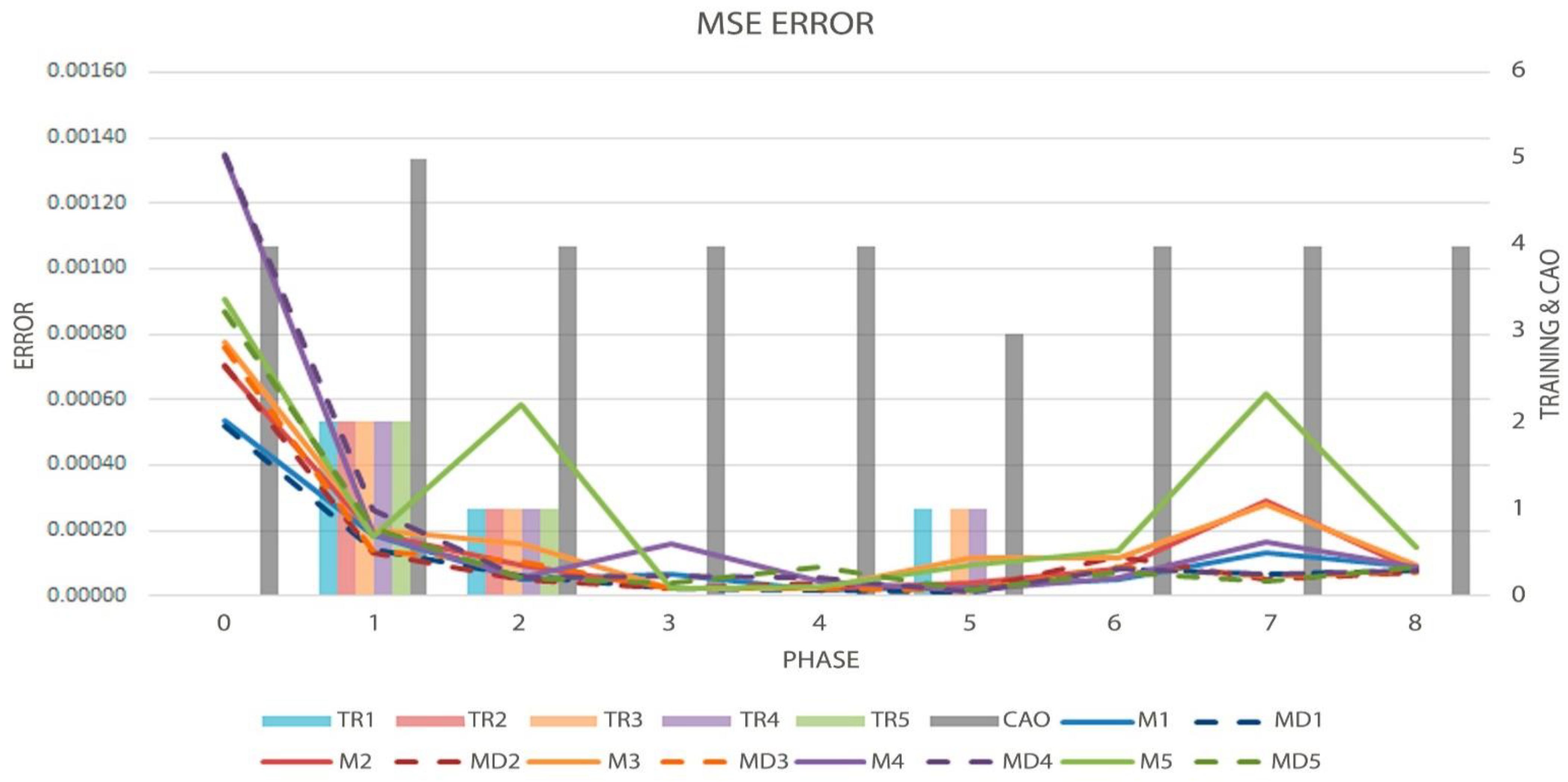
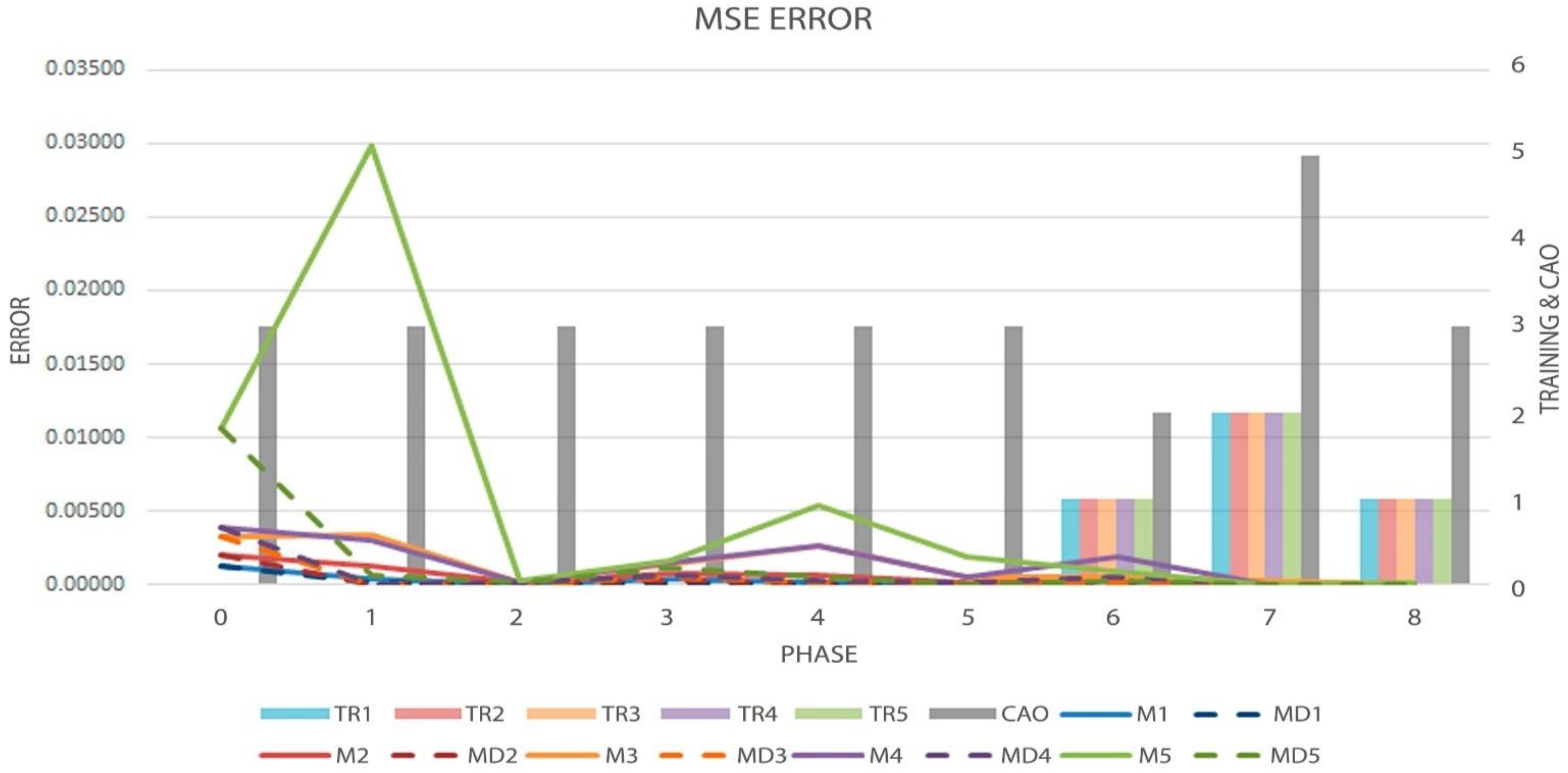
Figure 6.
Graph of the MSE metric (Solid and Dotted Lines, measured by left axis), Order evolution (CAO), and the decisions made by the algorithm (TR-Bars, the last two metrics measured by the right axis), in the first test.
Figure 6.
Graph of the MSE metric (Solid and Dotted Lines, measured by left axis), Order evolution (CAO), and the decisions made by the algorithm (TR-Bars, the last two metrics measured by the right axis), in the first test.
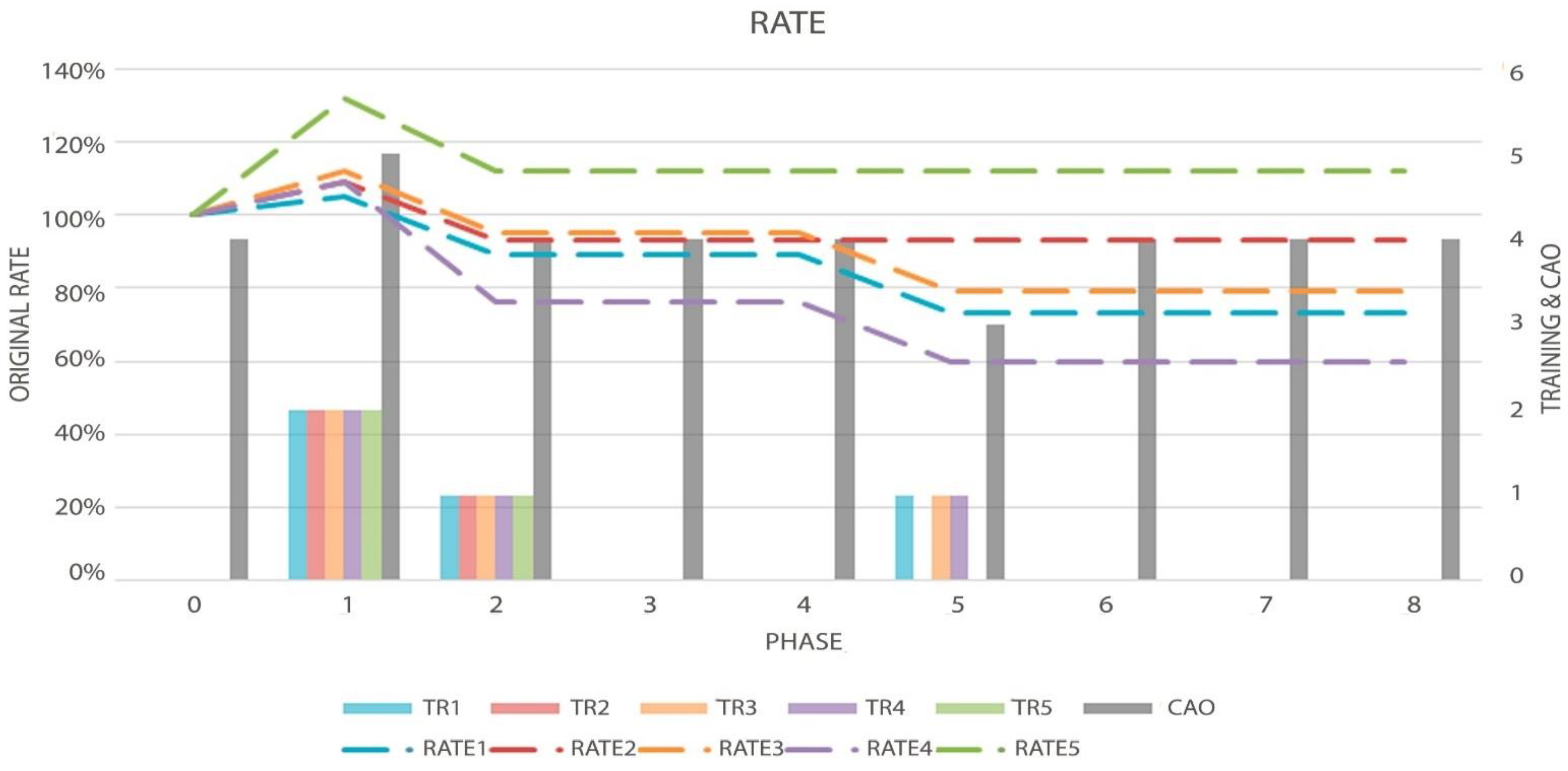
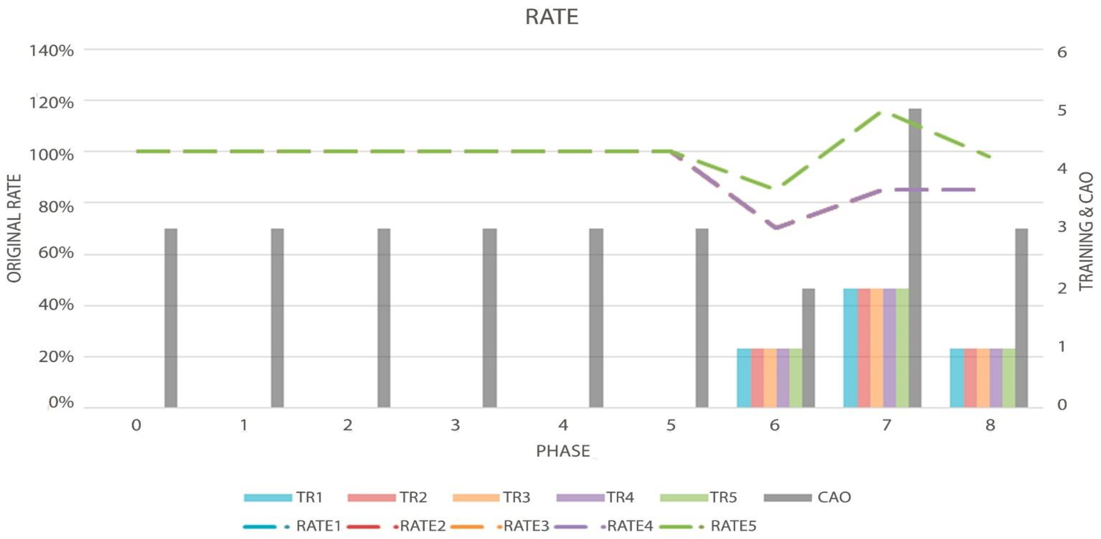
Figure 7.
Graph of the Topology Rate (Dotted Lines, measured by left axis), Order evolution (CAO), and the decisions made by the algorithm (TR-Bars, the last two metrics measured by the right axis) in the first test.
Figure 7.
Graph of the Topology Rate (Dotted Lines, measured by left axis), Order evolution (CAO), and the decisions made by the algorithm (TR-Bars, the last two metrics measured by the right axis) in the first test.
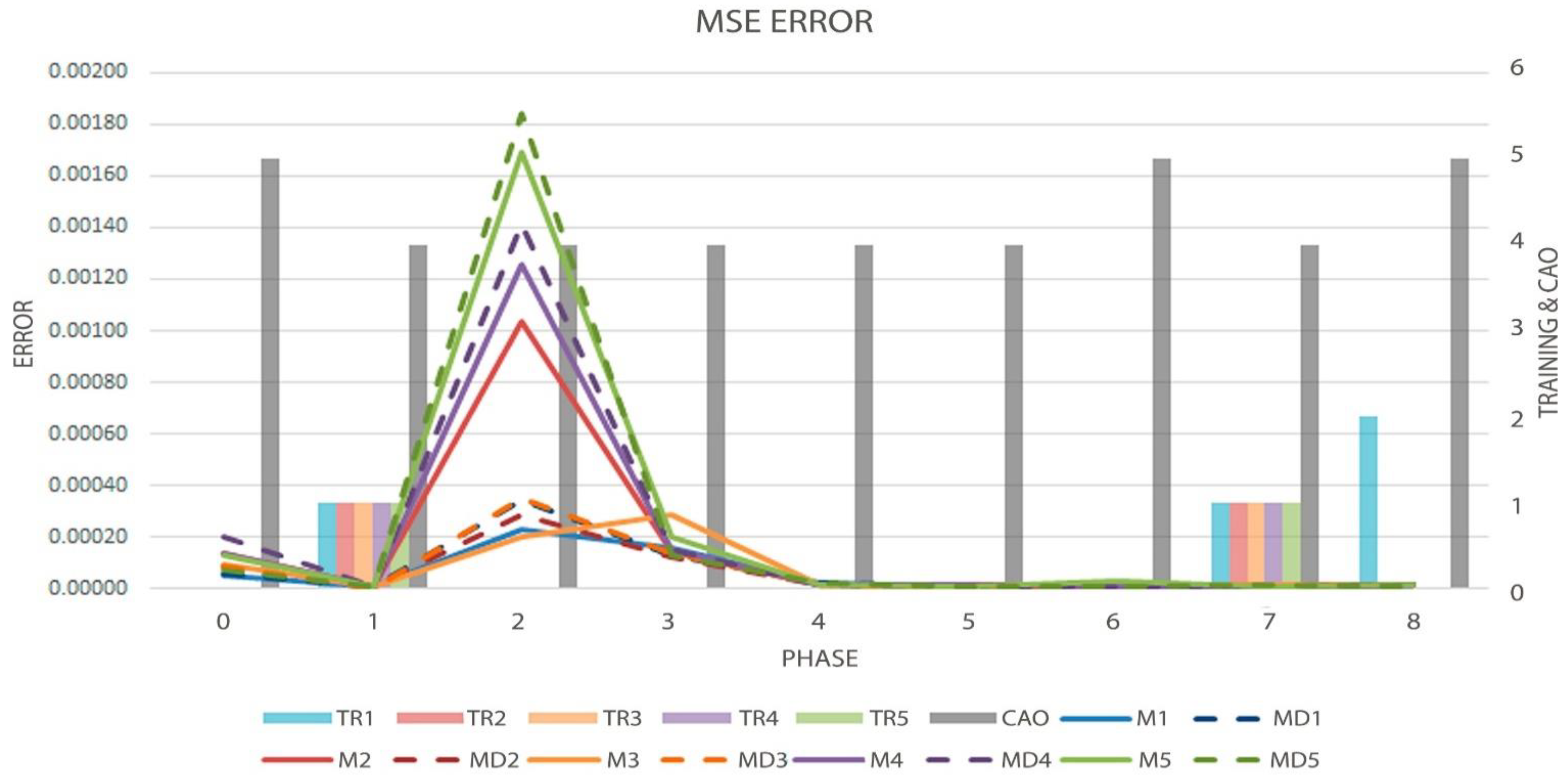
Figure 8.
Graph of the MSE metric (Solid and Dotted Lines, measured by left axis), Order evolution (CAO), and the decisions made by the algorithm (TR-Bars, the last two metrics measured by the right axis) in test eleven.
Figure 8.
Graph of the MSE metric (Solid and Dotted Lines, measured by left axis), Order evolution (CAO), and the decisions made by the algorithm (TR-Bars, the last two metrics measured by the right axis) in test eleven.
Figure 9.
Graph of the MSE metric (Solid and Dotted Lines, measured by left axis), Order evolution (CAO), and the decisions made by the algorithm (TR-Bars, the last two metrics measured by the right axis) in test five.
Figure 9.
Graph of the MSE metric (Solid and Dotted Lines, measured by left axis), Order evolution (CAO), and the decisions made by the algorithm (TR-Bars, the last two metrics measured by the right axis) in test five.
Figure 10.
Graph of the Topology Rate (Dotted Lines, measured by left axis), Order evolution (CAO), and the decisions made by the algorithm (TR-Bars, the last two metrics measured by the right axis) in test five.
Figure 10.
Graph of the Topology Rate (Dotted Lines, measured by left axis), Order evolution (CAO), and the decisions made by the algorithm (TR-Bars, the last two metrics measured by the right axis) in test five.
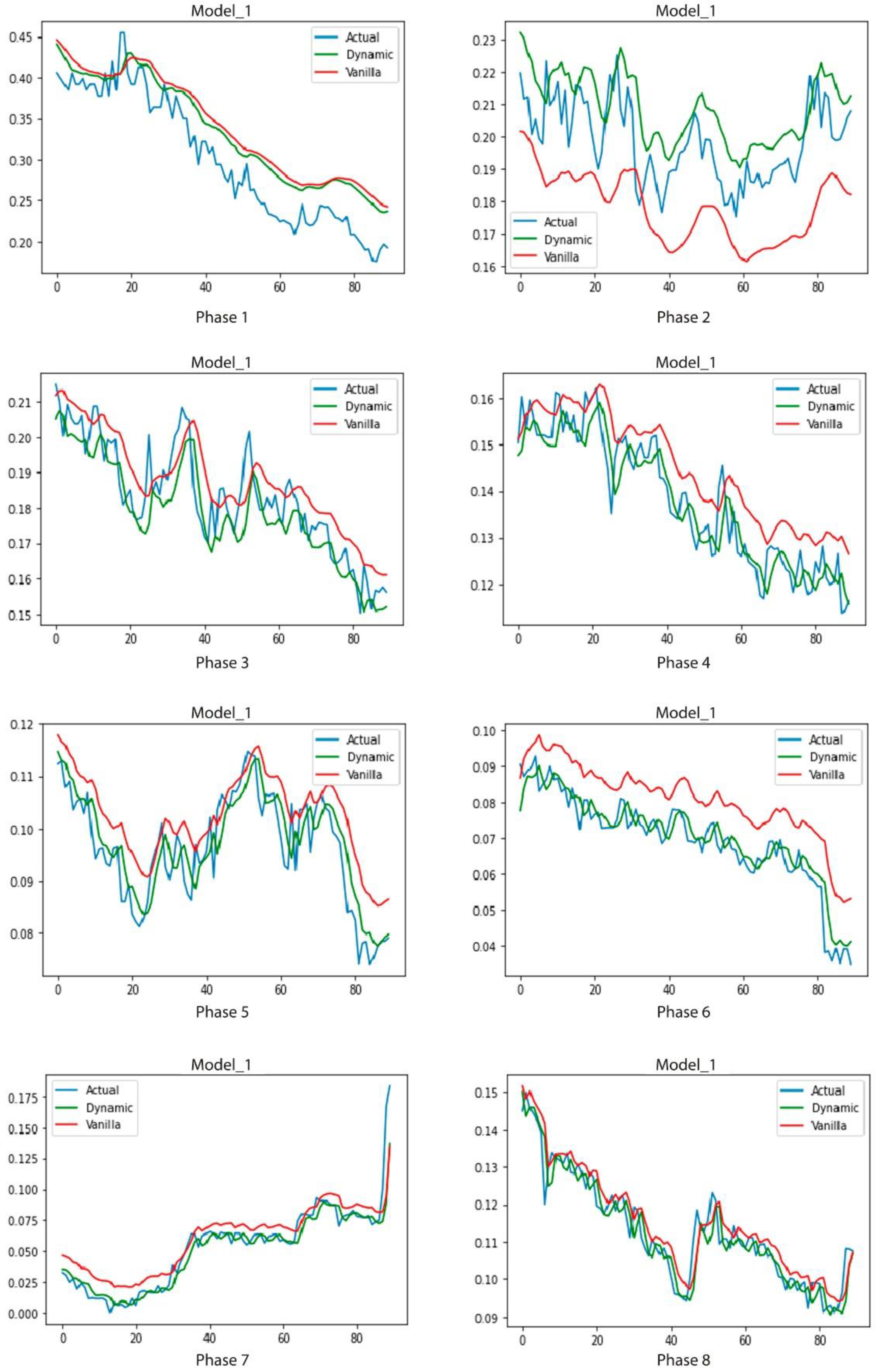
Figure 11.
Results of model 1 (Vanilla/DyLSTM) phases 1 to 8 in test four. Blue is the Actual timesereis, green is our proposed method and red is the vanilla model.
Figure 11.
Results of model 1 (Vanilla/DyLSTM) phases 1 to 8 in test four. Blue is the Actual timesereis, green is our proposed method and red is the vanilla model.
Table 1.
Decision-Making example by phases.
Table 1.
Decision-Making example by phases.
| Phase | 0 | 1 | 2 | 3 | 4 |
|---|
| Previous Decision | - | - | G | P | P, N |
| Error | | | | | |
| Error | - | - | > | > | < |
| Cao | 4 | 5 | 3 | 4 | 5 |
| Cao’s Suggest | - | G | P | G | G |
| Decision | - | G | P | N | G |
Table 2.
Models’ architecture.
Table 2.
Models’ architecture.
| Model | Layer 1 | Layer 2 | Layer Out |
|---|
| M1 | 64 | 32 | 1 |
| M2 | 32 | 16 | 1 |
| M3 | 24 | 12 | 1 |
| M4 | 18 | 6 | 1 |
| M5 | 9 | 5 | 1 |
Table 3.
Series 1 (MSE), order [Cao] and comparison between the 5 models [M] and their respective dynamic versions [MD], rate, and the decision made [TR] (Growth = 2, Pruning = 1, Normal = 0).
Table 3.
Series 1 (MSE), order [Cao] and comparison between the 5 models [M] and their respective dynamic versions [MD], rate, and the decision made [TR] (Growth = 2, Pruning = 1, Normal = 0).
MSE
MODEL | Phase 0 | Phase 1 | Phase 2 | Phase 3 | Phase 4 | Phase 5 | Phase 6 | Phase 7 | Phase 8 | AVG |
|---|
| M1 | 0.00053 | 0.00018 | 0.00005 | 0.00007 | 0.00002 | 0.00003 | 0.00005 | 0.00013 | 0.00009 | 0.00013 |
| MD1 | 0.00052 | 0.00015 | 0.00006 | 0.00002 | 0.00002 | 0.00001 | 0.00008 | 0.00007 | 0.00008 | 0.00011 |
| TR1 | 0 | 2 | 1 | 0 | 0 | 1 | 0 | 0 | 0 | |
| RATE 1 | 1 | 1.05 | 0.89 | 0.89 | 0.89 | 0.73 | 0.73 | 0.73 | 0.73 | |
| M2 | 0.00070 | 0.00019 | 0.00009 | 0.00002 | 0.00002 | 0.00004 | 0.00008 | 0.00029 | 0.00008 | 0.00017 |
| MD2 | 0.00070 | 0.00013 | 0.00005 | 0.00002 | 0.00004 | 0.00002 | 0.00012 | 0.00005 | 0.00007 | 0.00013 |
| TR2 | 0 | 2 | 1 | 0 | 0 | 0 | 0 | 0 | 0 | |
| RATE 2 | 1 | 1.09 | 0.93 | 0.93 | 0.93 | 0.93 | 0.93 | 0.93 | 0.93 | |
| M3 | 0.00078 | 0.00020 | 0.00016 | 0.00002 | 0.00002 | 0.00011 | 0.00011 | 0.00028 | 0.00010 | 0.00020 |
| MD3 | 0.00076 | 0.00014 | 0.00010 | 0.00002 | 0.00003 | 0.00002 | 0.00009 | 0.00006 | 0.00007 | 0.00014 |
| TR3 | 0 | 2 | 1 | 0 | 0 | 1 | 0 | 0 | 0 | |
| RATE 3 | 1 | 1.12 | 0.95 | 0.95 | 0.95 | 0.79 | 0.79 | 0.79 | 0.79 | |
| M4 | 0.00134 | 0.00019 | 0.00006 | 0.00016 | 0.00005 | 0.00002 | 0.00005 | 0.00017 | 0.00009 | 0.00024 |
| MD4 | 0.00135 | 0.00026 | 0.00006 | 0.00006 | 0.00005 | 0.00001 | 0.00008 | 0.00007 | 0.00008 | 0.00023 |
| TR4 | 0 | 2 | 1 | 0 | 0 | 1 | 0 | 0 | 0 | |
| RTE 4 | 1 | 1.09 | 0.76 | 0.76 | 0.76 | 0.6 | 0.6 | 0.6 | 0.6 | |
| M5 | 0.00091 | 0.00018 | 0.00059 | 0.00002 | 0.00003 | 0.00009 | 0.00014 | 0.00062 | 0.00015 | 0.00030 |
| MD5 | 0.00087 | 0.00021 | 0.00005 | 0.00004 | 0.00009 | 0.00002 | 0.00007 | 0.00005 | 0.00009 | 0.00016 |
| TR5 | 0 | 2 | 1 | 0 | 0 | 0 | 0 | 0 | 0 | |
| RATE 5 | 1 | 1.32 | 1.12 | 1.12 | 1.12 | 1.12 | 1.12 | 1.12 | 1.12 | |
| CAO | 4 | 5 | 4 | 4 | 4 | 3 | 4 | 4 | 4 | |
Table 4.
Series 1 (sMAPE), order [Cao], and comparison between the 5 models [M] and their respective dynamic versions [MD], rate, and the decision made [TR] (Growth = 2, Pruning = 1 Normal = 0).
Table 4.
Series 1 (sMAPE), order [Cao], and comparison between the 5 models [M] and their respective dynamic versions [MD], rate, and the decision made [TR] (Growth = 2, Pruning = 1 Normal = 0).
sMAPE
MODEL | Phase 0 | Phase 1 | Phase 2 | Phase 3 | Phase 4 | Phase 5 | Phase 6 | Phase 7 | Phase 8 | AVG |
|---|
| M1 | 37.97000 | 6.12000 | 2.13000 | 2.18000 | 0.77000 | 0.84000 | 0.78000 | 1.14000 | 0.84000 | 5.86333 |
| MD1 | 38.30000 | 4.41000 | 2.58000 | 1.06000 | 0.69000 | 0.58000 | 1.02000 | 0.79000 | 0.78000 | 5.57889 |
| TR1 | 0 | 2 | 1 | 0 | 0 | 1 | 0 | 0 | 0 | |
| RATE 1 | 1 | 1.05 | 0.89 | 0.89 | 0.89 | 0.73 | 0.73 | 0.73 | 0.73 | |
| M2 | 44.21000 | 6.23000 | 3.34000 | 1.04000 | 0.81000 | 1.03000 | 1.04000 | 1.81000 | 0.78000 | 6.69889 |
| MD2 | 44.00000 | 3.78000 | 2.21000 | 1.09000 | 1.17000 | 0.62000 | 1.30000 | 0.70000 | 0.75000 | 6.18000 |
| TR2 | 0 | 2 | 1 | 0 | 0 | 0 | 0 | 0 | 0 | |
| RATE 2 | 1 | 1.09 | 0.93 | 0.93 | 0.93 | 0.93 | 0.93 | 0.93 | 0.93 | |
| M3 | 47.29000 | 6.79000 | 4.55000 | 1.05000 | 0.81000 | 1.91000 | 1.28000 | 1.72000 | 0.86000 | 7.36222 |
| MD3 | 47.04000 | 3.81000 | 3.49000 | 1.07000 | 0.89000 | 0.60000 | 1.07000 | 0.75000 | 0.76000 | 6.60889 |
| TR3 | 0 | 2 | 1 | 0 | 0 | 1 | 0 | 0 | 0 | |
| RATE 3 | 1 | 1.12 | 0.95 | 0.95 | 0.95 | 0.79 | 0.79 | 0.79 | 0.79 | |
| M4 | 63.71000 | 6.28000 | 2.41000 | 3.37000 | 1.28000 | 0.68000 | 0.80000 | 1.28000 | 0.83000 | 8.96000 |
| MD4 | 63.80000 | 9.48000 | 2.48000 | 1.99000 | 1.36000 | 0.58000 | 1.03000 | 0.77000 | 0.76000 | 9.13889 |
| TR4 | 0 | 2 | 1 | 0 | 0 | 1 | 0 | 0 | 0 | |
| RATE 4 | 1 | 1.09 | 0.76 | 0.76 | 0.76 | 0.6 | 0.6 | 0.6 | 0.6 | |
| M5 | 50.64000 | 5.32000 | 8.64000 | 1.08000 | 1.00000 | 1.69000 | 1.41000 | 2.73000 | 1.07000 | 8.17556 |
| MD5 | 50.63000 | 7.11000 | 2.06000 | 1.50000 | 1.82000 | 0.58000 | 0.97000 | 0.66000 | 0.81000 | 7.34889 |
| TR5 | 0 | 2 | 1 | 0 | 0 | 0 | 0 | 0 | 0 | |
| RATE 5 | 1 | 1.32 | 1.12 | 1.12 | 1.12 | 1.12 | 1.12 | 1.12 | 1.12 | |
| CAO | 4 | 5 | 4 | 4 | 4 | 3 | 4 | 4 | 4 | |
Table 5.
Metric (OWA). Final percentage (RATE) of the topology with respect to the initial model. (New units) Number of extra units added.
Table 5.
Metric (OWA). Final percentage (RATE) of the topology with respect to the initial model. (New units) Number of extra units added.
| Model | OWA | RATE | New Units |
|---|
| M1/MD1 | 0.91 | 0.73 | 2 |
| M2/MD2 | 0.86 | 0.93 | 2 |
| M3/MD3 | 0.81 | 0.79 | 2 |
| M4/MD4 | 0.99 | 0.6 | 1 |
| M5/MD5 | 0.72 | 1.12 | 2 |
Table 6.
Cao’s method results from the 14 tests carried out.
Table 6.
Cao’s method results from the 14 tests carried out.
| | Phase 0 | Phase 1 | Phase 2 | Phase 3 | Phase 4 | Phase 5 | Phase 6 | Phase 7 | Phase 8 |
|---|
| CAO S1 | 4 | 5 | 4 | 4 | 4 | 3 | 4 | 4 | 4 |
| CAO S2 | 3 | 4 | 4 | 5 | 4 | 4 | 4 | 4 | 5 |
| CAO S3 | 4 | 4 | 4 | 5 | 5 | 5 | 4 | 5 | 5 |
| CAO S4 | 4 | 1 | 3 | 4 | 5 | 5 | 5 | 4 | 5 |
| CAO S5 | 3 | 3 | 3 | 3 | 3 | 3 | 2 | 5 | 3 |
| CAO S6 | 3 | 4 | 4 | 4 | 4 | 4 | 4 | 5 | 4 |
| CAO S7 | 4 | 4 | 4 | 4 | 3 | 4 | 4 | 5 | 4 |
| CAO S8 | 4 | 5 | 5 | 4 | 4 | 5 | 5 | 5 | 4 |
| CAO S9 | 4 | 4 | 4 | 4 | 4 | 5 | 4 | 4 | 5 |
| CAO S10 | 4 | 5 | 5 | 5 | 5 | 4 | 4 | 5 | 5 |
| CAO S11 | 5 | 4 | 4 | 4 | 4 | 4 | 5 | 4 | 5 |
| CAO S12 | 1 | 3 | 4 | 4 | 4 | 4 | 4 | 4 | 5 |
| CAO S13 | 1 | 5 | 4 | 4 | 4 | 4 | 4 | 4 | 4 |
| CAO S14 | 4 | 5 | 5 | 4 | 4 | 4 | 5 | 4 | 5 |
Table 7.
Results of the 14 tests carried out.
Table 7.
Results of the 14 tests carried out.
| MODEL | Serie 1 | Serie 2 | Serie 3 | Serie 4 | Serie 5 |
| OWA | RATE | UNITS + | OWA | RATE | UNITS + | OWA | RATE | UNITS + | OWA | RATE | UNITS + | OWA | RATE | UNITS + |
| M1/MD1 | 0.89 | 0.783 | 2 | 0.91 | 0.91 | 3 | 0.81 | 1.05 | 2 | 0.67 | 1.07 | 3 | 1.03 | 0.86 | 1 |
| M2/MD2 | 0.87 | 0.870
| 2 | 0.79 | 0.97 | 3 | 0.93 | 0.63 | 1 | 0.83 | 1.14 | 3 | 0.66 | 0.75 | 0 |
| M3/MD3 | 0.79 | 0.790
| 2 | 0.79 | 0.99 | 3 | 0.90 | 0.69 | 1 | 0.88 | 1.27 | 4 | 0.67 | 0.76 | 1 |
| M4/MD4 | 0.76 | 0.763
| 1 | 0.61 | 1.05 | 3 | 0.88 | 0.80 | 1 | 0.97 | 1.40 | 4 | 0.59 | 0.82 | 1 |
| M5/MD5 | 0.94 |
0.937
| 2 | 0.86 | 1.23 | 3 | 1.07 | 0.98 | 1 | 1.03 | 1.78 | 4 | 0.38 | 0.79 | 1 |
| MODEL | Serie 6 | Serie 7 | Serie 8 | Serie 9 | Serie 10 |
| OWA | RATE | UNITS + | OWA | RATE | UNITS + | OWA | RATE | UNITS + | OWA | RATE | UNITS + | OWA | RATE | UNITS + |
| M1/MD1 | 0.94 | 1.05 | 2 | 0.84 | 0.50 | 0 | 0.96 | 0.87 | 1 | 0.80 | 0.87 | 1 | 0.81 | 0.88 | 2 |
| M2/MD2 | 0.90 | 1.09 | 2 | 0.88 | 0.51 | 0 | 0.96 | 0.98 | 2 | 0.76 | 0.89 | 1 | 0.89 | 0.93 | 2 |
| M3/MD3 | 0.90 | 1.12 | 2 | 0.90 | 0.74 | 1 | 0.92 | 0.89 | 2 | 0.77 | 0.90 | 1 | 0.86 | 0.95 | 2 |
| M4/MD4 | 0.92 | 1.18 | 2 | 0.88 | 0.87 | 0 | 0.80 | 1.01 | 2 | 0.85 | 0.93 | 1 | 0.94 | 1.05 | 2 |
| M5/MD5 | 0.89 | 1.31 | 2 | 0.94 | 0.74 | 0 | 0.94 | 1.10 | 2 | 0.82 | 0.97 | 1 | 0.82 | 1.38 | 2 |
| MODEL | Serie 11 | Serie 12 | Serie 13 | Serie 14 | |
| OWA | RATE | UNITS + | OWA | RATE | UNITS + | OWA | RATE | UNITS + | OWA | RATE | UNITS + | | | |
| M1/MD1 | 1.01 | 0.70 | 0 | 0.60 | 1.05 | 2 | 0.67 | 0.89 | 2 | 0.99 | 0.73 | 2 | | | |
| M2/MD2 | 0.75 | 0.60 | 0 | 0.70 | 1.09 | 2 | 0.72 | 0.87 | 2 | 1.01 | 0.76 | 2 | | | |
| M3/MD3 | 1.03 | 0.55 | 0 | 0.58 | 1.12 | 2 | 0.60 | 0.95 | 2 | 0.87 | 0.79 | 2 | | | |
| M4/MD4 | 1.01 | 0.55 | 0 | 0.51 | 1.17 | 2 | 0.49 | 0.88 | 2 | 0.94 | 0.77 | 2 | | | |
| M5/MD5 | 0.66 | 0.40 | 0 | 0.56 | 1.27 | 2 | 0.60 | 0.99 | 2 | 0.91 | 0.95 | 2 | | | |
Table 8.
Series 11 (MSE), order [Cao], and comparison between the 5 models [M] and their respective dynamic versions [MD], rate, and the decision made [TR] (Growth = 2, Pruning = 1 Normal = 0).
Table 8.
Series 11 (MSE), order [Cao], and comparison between the 5 models [M] and their respective dynamic versions [MD], rate, and the decision made [TR] (Growth = 2, Pruning = 1 Normal = 0).
MSE
MODEL | Phase 0 | Phase 1 | Phase 2 | Phase 3 | Phase 4 | Phase 5 | Phase 6 | Phase 7 | Phase 8 | AVG |
|---|
| M1 | 0.00005 | 0.00001 | 0.00023 | 0.00015 | 0.00002 | 0.00001 | 0.00001 | 0.00001 | 0.00001 | 0.00006 |
| MD1 | 0.00006 | 0.00001 | 0.00035 | 0.00013 | 0.00002 | 0.00001 | 0.00001 | 0.00001 | 0.00001 | 0.00007 |
| TR1 | 0 | 1 | 0 | 0 | 0 | 0 | 0 | 1 | 2 | |
| RATE 1 | 1 | 0.85 | 0.85 | 0.85 | 0.85 | 0.85 | 0.85 | 0.7 | 0.85 | |
| M2 | 0.00014 | 0.00001 | 0.00104 | 0.00014 | 0.00002 | 0.00001 | 0.00002 | 0.00001 | 0.00002 | 0.00015 |
| MD2 | 0.00008 | 0.00001 | 0.00029 | 0.00012 | 0.00002 | 0.00001 | 0.00001 | 0.00001 | 0.00001 | 0.00006 |
| TR2 | 0 | 1 | 0 | 0 | 0 | 0 | 0 | 1 | 0 | |
| RATE 2 | 1 | 0.7 | 0.7 | 0.7 | 0.7 | 0.7 | 0.7 | 0.55 | 0.55 | |
| M3 | 0.00009 | 0.00000 | 0.00020 | 0.00029 | 0.00002 | 0.00001 | 0.00001 | 0.00001 | 0.00001 | 0.00007 |
| MD3 | 0.00009 | 0.00000 | 0.00035 | 0.00014 | 0.00002 | 0.00001 | 0.00001 | 0.00001 | 0.00001 | 0.00007 |
| TR3 | 0 | 1 | 0 | 0 | 0 | 0 | 0 | 1 | 0 | |
| RATE 3 | 1 | 0.55 | 0.55 | 0.55 | 0.55 | 0.55 | 0.55 | 0.4 | 0.4 | |
| M4 | 0.00014 | 0.00001 | 0.00126 | 0.00015 | 0.00001 | 0.00001 | 0.00001 | 0.00001 | 0.00001 | 0.00018 |
| MD4 | 0.00020 | 0.00001 | 0.00141 | 0.00015 | 0.00002 | 0.00001 | 0.00001 | 0.00001 | 0.00001 | 0.00020 |
| TR4 | 0 | 1 | 0 | 0 | 0 | 0 | 0 | 1 | 0 | |
| RATE 4 | 1 | 0.7 | 0.7 | 0.7 | 0.7 | 0.7 | 0.7 | 0.55 | 0.55 | |
| M5 | 0.00013 | 0.00000 | 0.00169 | 0.00020 | 0.00002 | 0.00001 | 0.00003 | 0.00001 | 0.00001 | 0.00023 |
| MD5 | 0.00008 | 0.00001 | 0.00184 | 0.00013 | 0.00002 | 0.00001 | 0.00001 | 0.00002 | 0.00001 | 0.00023 |
| TR5 | 0 | 1 | 0 | 0 | 0 | 0 | 0 | 1 | 0 | |
| RATE 5 | 1 | 0.55 | 0.55 | 0.55 | 0.55 | 0.55 | 0.55 | 0.4 | 0.4 | |
| CAO |
5
|
4
|
4
|
4
|
4
|
4
|
5
|
4
|
5
| |
Table 9.
Metric (OWA). Final percentage (RATE) of the topology with respect to the initial model. (New units) Number of extra units added, test eleven.
Table 9.
Metric (OWA). Final percentage (RATE) of the topology with respect to the initial model. (New units) Number of extra units added, test eleven.
| Model | OWA | RATE | NEW Units |
|---|
| M1/MD1 | 1.11 | 0.85 | 0 |
| M2/MD2 | 0.54 | 0.55 | 0 |
| M3/MD3 | 0.93 | 0.4 | 0 |
| M4/MD4 | 1.03 | 0.55 | 0 |
| M5/MD5 | 0.87 | 0.4 | 0 |
Table 10.
Series 5 (MSE), order [Cao] and comparison between the 5 models [M] and their respective dynamic versions [MD], rate, and the decision made [TR] (Growth = 2, Pruning = 1 Normal = 0).
Table 10.
Series 5 (MSE), order [Cao] and comparison between the 5 models [M] and their respective dynamic versions [MD], rate, and the decision made [TR] (Growth = 2, Pruning = 1 Normal = 0).
MSE
MODEL | Phase 0 | Phase 1 | Phase 2 | Phase 3 | Phase 4 | Phase 5 | Phase 6 | Phase 7 | Phase 8 | AVG |
|---|
| M1 | 0.00123 | 0.00034 | 0.00007 | 0.00034 | 0.00017 | 0.00003 | 0.00027 | 0.00003 | 0.00001 | 0.00028 |
| MD1 | 0.00128 | 0.00017 | 0.00006 | 0.00015 | 0.00005 | 0.00004 | 0.00007 | 0.00002 | 0.00005 | 0.00021 |
| TR1 | 0 | 0 | 0 | 0 | 0 | 0 | 1 | 2 | 1 | |
| RATE 1 | 1 | 1 | 1 | 1 | 1 | 1 | 0.7 | 0.85 | 0.85 | |
| M2 | 0.00196 | 0.00131 | 0.00008 | 0.00081 | 0.00061 | 0.00012 | 0.00022 | 0.00002 | 0.00001 | 0.00057 |
| MD2 | 0.00195 | 0.00005 | 0.00009 | 0.00029 | 0.00012 | 0.00007 | 0.00008 | 0.00009 | 0.00001 | 0.00031 |
| TR2 | 0 | 0 | 0 | 0 | 0 | 0 | 1 | 2 | 1 | |
| RATE 2 | 1 | 1 | 1 | 1 | 1 | 1 | 0.7 | 0.85 | 0.85 | |
| M3 | 0.00331 | 0.00339 | 0.00008 | 0.00134 | 0.00259 | 0.00054 | 0.00050 | 0.00026 | 0.00004 | 0.00134 |
| MD3 | 0.00326 | 0.00005 | 0.00007 | 0.00046 | 0.00015 | 0.00009 | 0.00015 | 0.00003 | 0.00001 | 0.00048 |
| TR3 | 0 | 0 | 0 | 0 | 0 | 0 | 1 | 2 | 1 | |
| RATE 3 | 1 | 1 | 1 | 1 | 1 | 1 | 0.7 | 0.85 | 0.85 | |
| M4 | 0.00389 | 0.00307 | 0.00010 | 0.00146 | 0.00267 | 0.00057 | 0.00192 | 0.00002 | 0.00002 | 0.00152 |
| MD4 | 0.00386 | 0.00005 | 0.00008 | 0.00064 | 0.00029 | 0.00016 | 0.00055 | 0.00002 | 0.00001 | 0.00063 |
| TR4 | 0 | 0 | 0 | 0 | 0 | 0 | 1 | 2 | 1 | |
| RATE 4 | 1 | 1 | 1 | 1 | 1 | 1 | 0.7 | 0.85 | 0.85 | |
| M5 | 0.01068 | 0.02985 | 0.00021 | 0.00160 | 0.00532 | 0.00189 | 0.00082 | 0.00002 | 0.00008 | 0.00561 |
| MD5 | 0.01063 | 0.00061 | 0.00012 | 0.00113 | 0.00056 | 0.00004 | 0.00027 | 0.00002 | 0.00002 | 0.00149 |
| TR5 | 0 | 0 | 0 | 0 | 0 | 0 | 1 | 2 | 1 | |
| RATE 5 | 1 | 1 | 1 | 1 | 1 | 1 | 0.85 | 1.16 | 0.98 | |
| CAO | 3 | 3 | 3 | 3 | 3 | 3 | 2 | 5 | 3 | |
Table 11.
Series 4 (MSE), order [Cao], and comparison between the 5 models [M] and their respective dynamic versions [MD], rate, and the decision made [TR] (Growth = 2, Pruning = 1 Normal = 0).
Table 11.
Series 4 (MSE), order [Cao], and comparison between the 5 models [M] and their respective dynamic versions [MD], rate, and the decision made [TR] (Growth = 2, Pruning = 1 Normal = 0).
MSE
MODEL | Phase 0 | Phase 1 | Phase 2 | Phase 3 | Phase 4 | Phase 5 | Phase 6 | Phase 7 | Phase 8 | AVG |
|---|
| M1 | 0.00047 | 0.00216 | 0.00051 | 0.00008 | 0.00008 | 0.00007 | 0.00015 | 0.00022 | 0.00003 | 0.00042 |
| MD1 | 0.00055 | 0.00162 | 0.00017 | 0.00007 | 0.00003 | 0.00002 | 0.00002 | 0.00014 | 0.00002 | 0.00029 |
| TR1 | 0 | 1 | 2 | 2 | 2 | 0 | 0 | 0 | 0 | |
| RATE 1 | 1 | 0.85 | 1.02 | 1.05 | 1.07 | 1.07 | 1.07 | 1.07 | 1.07 | |
| M2 | 0.00051 | 0.00328 | 0.00035 | 0.00016 | 0.00015 | 0.00018 | 0.00002 | 0.00018 | 0.00003 | 0.00054 |
| MD2 | 0.00048 | 0.00287 | 0.00059 | 0.00006 | 0.00075 | 0.00005 | 0.00002 | 0.00015 | 0.00002 | 0.00055 |
| TR2 | 0 | 1 | 2 | 2 | 2 | 0 | 0 | 0 | 0 | |
| RATE 2 | 1 | 0.7 | 1.04 | 1.09 | 1.19 | 1.19 | 1.19 | 1.19 | 1.19 | |
| M3 | 0.00047 | 0.00281 | 0.00012 | 0.00006 | 0.00005 | 0.00005 | 0.00002 | 0.00017 | 0.00002 | 0.00042 |
| MD3 | 0.00046 | 0.00213 | 0.00033 | 0.00006 | 0.00009 | 0.00002 | 0.00002 | 0.00016 | 0.00002 | 0.00037 |
| TR3 | 0 | 1 | 2 | 2 | 2 | 0 | 0 | 0 | 0 | |
| RATE 3 | 1 | 0.7 | 1.06 | 1.19 | 1.32 | 1.32 | 1.32 | 1.32 | 1.32 | |
| M4 | 0.00059 | 0.00447 | 0.00011 | 0.00020 | 0.00017 | 0.00004 | 0.00004 | 0.00026 | 0.00003 | 0.00066 |
| MD4 | 0.00057 | 0.00403 | 0.00077 | 0.00008 | 0.00003 | 0.00003 | 0.00002 | 0.00014 | 0.00002 | 0.00063 |
| TR4 | 0 | 1 | 2 | 2 | 2 | 0 | 0 | 0 | 0 | |
| RATE 4 | 1 | 0.85 | 1.13 | 1.23 | 1.43 | 1.43 | 1.43 | 1.43 | 1.43 | |
| M5 | 0.00194 | 0.00326 | 0.00057 | 0.00011 | 0.00030 | 0.00030 | 0.00006 | 0.00026 | 0.00003 | 0.00076 |
| MD5 | 0.00180 | 0.00349 | 0.00081 | 0.00012 | 0.00017 | 0.00006 | 0.00003 | 0.00016 | 0.00003 | 0.00074 |
| TR5 | 0 | 1 | 2 | 2 | 2 | 0 | 0 | 0 | 0 | |
| RATE 5 | 1 | 0.85 | 1.16 | 1.32 | 1.65 | 1.65 | 1.65 | 1.65 | 1.65 | |
| CAO |
4
|
1
|
3
|
4
|
5
|
5
|
5
|
4
|
5
| |
Table 12.
Metric (OWA). Final percentage (RATE) of the topology with respect to the initial model. (New units) Number of extra units added, test four.
Table 12.
Metric (OWA). Final percentage (RATE) of the topology with respect to the initial model. (New units) Number of extra units added, test four.
| Model | OWA | RATE | New Units |
|---|
| M1/MD1 | 0.65 | 1.07 | 3 |
| M2/MD2 | 0.99 | 1.19 | 4 |
| M3/MD3 | 0.91 | 1.32 | 5 |
| M4/MD4 | 0.93 | 1.43 | 5 |
| M5/MD5 | 0.89 | 1.65 | 4 |


