Multi-Guide Set-Based Particle Swarm Optimization for Multi-Objective Portfolio Optimization

Abstract

Portfolio optimization is a multi-objective optimization problem (MOOP) with risk and profit, or some form of the two, as competing objectives. Single-objective portfolio optimization requires a trade-off coefficient to be specified in order to balance the two objectives. Erwin and Engelbrecht proposed a set-based approach to single-objective portfolio optimization, namely, set-based particle swarm optimization (SBPSO). SBPSO selects a sub-set of assets that form a search space for a secondary optimization task to optimize the asset weights. The authors found that SBPSO was able to identify good solutions to portfolio optimization problems and noted the benefits of redefining the portfolio optimization problem as a set-based problem. This paper proposes the first multi-objective optimization (MOO) approach to SBPSO, and its performance is investigated for multi-objective portfolio optimization. Alongside this investigation, the performance of multi-guide particle swarm optimization (MGPSO) for multi-objective portfolio optimization is evaluated and the performance of SBPSO for portfolio optimization is compared against multi-objective algorithms. It is shown that SBPSO is as competitive as multi-objective algorithms, albeit with multiple runs. The proposed multi-objective SBPSO, i.e., multi-guide set-based particle swarm optimization (MGSBPSO), performs similarly to other multi-objective algorithms while obtaining a more diverse set of optimal solutions.

1. Introduction

Portfolio optimization is a complex problem not only in the depth of the topics that it covers, but also in its breadth. It is the process of determining which assets to include in a portfolio while simultaneously maximizing profit and minimizing risk. To illustrate the investment process, consider the game of Monopoly. In the game, players purchase property. When a player lands on another player’s property, that player must then pay the owner a fee. The more expensive the property purchased is, the higher the fees will be. Players must, therefore, strategize about which properties to buy. In some cases, a player might take a risk and purchase an expensive property, but unfortunately, it is hardly ever visited by other players. In this scenario, the risk does not pay off and possibly jeopardizes the player’s position in the game. Players must determine what the best possible way to spend their money would be in order to maximize their profits without going bankrupt.

The real world is much more complex, with many moving parts, but it is similar to Monopoly in that investing can be a risky venture. However, it is possible that an asset’s value increases significantly, making it a worthwhile investment. Identifying which asset or collection of assets—known as a portfolio—would yield an optimal balance between risk and reward is not an easy task. Moreover, there may exist multiple, but equally good, portfolios that have different risk and return characteristics, which further complicates the task. Lastly, when constraints that introduce nonlinearity and non-convexity (such as boundary constraints and cardinality constraints) are added, the problem becomes NP-Hard [1,2,3]. Thus, approaches such as quadratic programming cannot be efficiently utilized to obtain solutions.

Meta-heuristics are computationally efficient and are effective approaches to obtaining good-quality solutions for a variety of portfolio models [3]. Typically, solutions are represented by fixed-length vectors of floats where the elements in a vector correspond to asset weights. Unfortunately, the performance of fixed-length vector meta-heuristics deteriorate for larger portfolio optimization problems [4]. An alternative approach is to redefine the portfolio problem as a set-based problem where a subset of assets are selected and then the weights of these assets are optimized. For example, hybridization approaches that integrate quadratic programming with genetic algorithms (GAs) have been shown to increase performance for constrained portfolio optimization problems [5,6,7,8,9]. A new set-based approach, set-based particle swarm optimization (SBPSO) for portfolio optimization, uses particle swarm optimization (PSO) to optimize asset weights instead of quadratic programming and has demonstrated good performance for the portfolio optimization problem [10].

Single-objective portfolio optimization requires a trade-off coefficient to be specified in order to balance the two objectives, i.e., risk and return. A collection of equally good but different solutions can then be obtained by solving the single-objective optimization problem for various trade-off coefficient values. However, a more sophisticated and appropriate approach would be to use a multi-objective optimization (MOO) algorithm to identify an equally spread set of non-dominated solutions, e.g., multi-guide particle swarm optimization (MGPSO). MGPSO is a multi-swarm multi-objective PSO algorithm that uses a shared archive to store non-dominated solutions found by the swarms [11].

This paper proposes a new approach to multi-objective portfolio optimization, multiguide set-based particle swarm optimization (MGSBPSO), that combines elements of SBPSO with MGPSO. The novelty of the proposed approach is that it can identify multiple but equally good solutions to the portfolio optimization problem with the scaling benefits of a set-based approach. Furthermore, the proposed approach identifies subsets of assets to be included in the portfolio, leading to a reduction in the dimensionality of the problem. Lastly, MGSBPSO is the first MOO approach to SBPSO.

The performance of MGSBPSO for portfolio optimization is investigated and compared with that of other multi-objective algorithms, namely, MGPSO, non-dominated sorting genetic algorithm II (NSGA-II) [12], and strength Pareto evolutionary algorithm 2 (SPEA2) [13]. The single-objective SBPSO is also included in the performance comparisons as a baseline benchmark and to evaluate whether SBPSO is competitive amongst multi-objective algorithms. NSGA-II and SPEA2 were selected to compare with MGSBPSO, since these algorithms had been used extensively for portfolio optimization before [14,15,16,17,18,19,20]. It should also be noted that this paper is the first to apply MGPSO to the portfolio optimization problem.

The main findings of this paper are:

• MGSBPSO is capable of identifying non-dominated solutions to several portfolio optimization problems of varying dimensionalities.
• The single-objective SBPSO can obtain results (over a number of runs) that are just as good as those obtained by multi-objective algorithms.
• NSGA-II and SPEA2 obtain good-quality solutions, although they are not as diverse as the solutions found by SBPSO, MGPSO, and MGSBPSO.
• MGPSO using a tuning-free approach [21] performs similarly to NSGA-II and SPEA2 using tuned control parameter values.
• MGSBPSO scales to larger portfolio problems better than MGPSO, NSGA-II, and SPEA2.

The remainder of this paper is organized as follows: The necessary background for the portfolio optimization is given in Section 2. Section 3 details the algorithms used in this paper. Section 4 proposes MGSBPSO for portfolio optimization. The empirical process for determining the performance of the proposed approach is explained in Section 5, and the results are presented in Section 6. Section 7 concludes the paper. Ideas for future work are given in Section 8.

2. Portfolio Optimization

The objective of an optimization problem is to find a solution such that a given quantity is optimized, possibly subject to a set of constraints [22]. Portfolio optimization is a problem in which profit and risk are optimized—either as a single-objective optimization problem or a multi-objective optimization problem.

This section presents the necessary background on optimization and portfolio optimization needed for this paper. Section 2.1 and Section 2.2 briefly discuss single- and multi-objective optimization, respectively. Section 2.3 discusses portfolio optimization.

2.1. Single-Objective Optimization

Formally, a boundary-constrained single-objective optimization problem, f, assuming minimization, is defined as

$$\begin{array}{cc}\hfill \mathrm{m}\mathrm{i}\mathrm{n}\mathrm{i}\mathrm{m}\mathrm{i}\mathrm{z}\mathrm{e}& f\left(\mathit{x}\right),\mathit{x}=(x_1,x_2,\dots ,x_n)\hfill \\ \hfill & \mathit{x}\in \mathsf{\Omega }\hfill \end{array}$$

(1)

where $\mathit{x}$ is an n-dimensional decision vector within the search space, $\mathsf{\Omega }$ [22]. Each point in the decision vector corresponds to a decision variable in f. Solutions to f are constrained to the bounds of $\mathsf{\Omega }$.

2.2. Multi-Objective Optimization

A multi-objective optimization problem (MOOP) is the simultaneous optimization of two or three conflicting objectives [22]. Assuming minimization, multi-objective and many-objective optimization problems are defined as

$$\begin{array}{cc}\hfill \mathrm{m}\mathrm{i}\mathrm{n}\mathrm{i}\mathrm{m}\mathrm{i}\mathrm{z}\mathrm{e}& f\left(\mathit{x}\right)=(f_1\left(\mathit{x}\right),f_2\left(\mathit{x}\right),\dots ,f_m\left(\mathit{x}\right))\hfill \\ \hfill & \mathit{x}\in \mathsf{\Omega }\hfill \end{array}$$

(2)

where m is the number of objectives.

There may exist multiple equally good solutions to a MOOP. These solutions, which are vectors in the decision space, balance the multiple objectives and can be seen as a set of optimal trade-offs to the problem. This set is formally referred to as Pareto-optimal solutions (POS). The POS are mapped to the objective space (by evaluating the multiple objectives functions) to the objective space. This new set of solutions in the objective space are formally referred to as the Pareto-optimal front (POF). The solutions in the POF are not dominated by any other feasible solution. A decision vector ${\mathit{x}}_1$ in the objective space dominates another decision vector ${\mathit{x}}_2$ in the objective space, expressed as ${\mathit{x}}_1\prec {\mathit{x}}_2$, if and only if $f_k\left({\mathit{x}}_1\right)\le f_k\left({\mathit{x}}_2\right)\forall k\in \{1,\dots ,m\}$ and $\exists k\in \{1,\dots ,m\}$ such that $f_k\left({\mathit{x}}_1\right)<f_k\left({\mathit{x}}_2\right)$, assuming a minimization problem. Multi-objective optimization algorithms search for a diverse set of solutions that are as close to the true POF as possible [22].

2.3. Mean-Variance Portfolio Optimization

A portfolio model is a mathematical description of the behavior of a portfolio of assets given market-related information. The portfolio model is optimized, typically, by adjusting the weights of the assets in the portfolio. A popular portfolio model is the mean-variance model, which is formally defined as

$$\mathrm{m}\mathrm{i}\mathrm{n}\mathrm{i}\mathrm{m}\mathrm{i}\mathrm{z}\mathrm{e}\lambda \overline{\sigma }-(1-\lambda )R$$

(3)

where $\lambda$ is used to balance risk ($\overline{\sigma }$) and return (R). The $\lambda$ coefficient is bound in $[0,1]$, where smaller values favor return and larger values favor risk. Risk is calculated as the weighted covariance between all n assets in the portfolio:

$$\overline{\sigma }=\sum _{i=1}^n\sum _{j=1}^n{w}_i{w}_j{\sigma }_{ij}$$

(4)

where $w_i$ and $w_j$ are weightings of assets i and j, respectively, and ${\sigma }_{ij}$ is the covariance between assets i and j. R is calculated using

$$R=\sum _{i=1}^n{R}_i{w}_i$$

(5)

where $R_i$ is the return of asset i.

The mean-variance model is subject to two constraints: (1) The summation of all asset weights must be equal to one, and (2) the weight of each asset must be non-negative. These constraints are expressed as

$$\sum _{i=1}^n{w}_i=1,$$

(6)

and

$$w_i\ge 0.$$

(7)

The mean-variance model (Equation (3)) is optimized by tuning the weights, i.e., $w$, to return the lowest value for a given $\lambda$ value. A diverse set of optimal portfolios can be obtained by repeating the optimization process for different $\lambda$ values. Multi-objective portfolio optimization, however, is the simultaneous maximization of return (Equation (5)) and minimization of risk (Equation (4)) by tuning the weights to balance these conflicting objectives.

3. Optimization Algorithms for Portfolio Optimization

There have been many applications of optimization algorithms to both the single-objective and multi-objective portfolio optimization problems [3]. This section presents a subset of meta-heuristics that have been applied to portfolio optimization. Section 3.1 introduces PSO—a popular approach to single-objective portfolio optimization. Set-based particle swarm optimization, a recently proposed approach to single-objective optimization [10], is explained in Section 3.2. Multi-guide particle swarm optimization (this paper is the first to apply MGPSO to multi-objective portfolio optimization) is discussed in Section 3.3. Section 3.4 and Section 3.5 present NSGA-II and SPEA2, respectively, which have previously been applied to multi-objective portfolio optimization [14,15,16,17,18,19,20].

3.1. Particle Swarm Optimization

PSO, which was first proposed in 1995 by Eberhart and Kennedy, is a single-objective optimization algorithm [23]. The algorithm iteratively updates its collection of particles (referred to as a swarm) to find solutions to the optimization problem under consideration. The position of a particle, which is randomly initialized, is a candidate solution to the problem. In the case of portfolio optimization, the position of a particle represents the weights used in the calculation of Equation (3). Each particle also has a velocity (initially a vector of zeros) that guides the particle to more promising areas of the search space. The position of a particle is updated with their velocity at each time step t to produce a new candidate solution. The velocity of a particle is influenced by the previous velocity of the particle and social and cognitive guides. The cognitive guide is a particle’s personal best-known solution that has been found thus far, and the social guide is the best-known solution found thus far within a neighborhood (network) of particles. A global network means that the social guide is the best-known solution found by the entire swarm thus far, which is what is used in this paper. This paper also uses an inertia-weighted velocity update to regulate the trade-off between exploitation and exploration [24]. The velocity update is defined as

$$\begin{array}{c}{\mathit{v}}_i(t+1)=w{\mathit{v}}_i\left(t\right)+c_1{\mathit{r}}_{1,i}\left(t\right)({\mathit{y}}_i\left(t\right)-{\mathit{x}}_i\left(t\right))c_2{\mathit{r}}_{2,i}\left(t\right)({\widehat{\mathit{y}}}_i\left(t\right)-{\mathit{x}}_i\left(t\right))\end{array}$$

(8)

where ${\mathit{v}}_i$ is the velocity of particle i; w is the inertia weight; $c_1$ and $c_2$ are acceleration coefficients that control the influence of the cognitive and social guides, respectively; ${\mathit{r}}_1$ and ${\mathit{r}}_2$ are vectors of random values sampled from a standard uniform distribution in the range [0, 1]; ${\mathit{y}}_i$ is the cognitive guide of particle i; ${\widehat{\mathit{y}}}_i$ is the social guide of particle i. A particle’s position is updated using

$${\mathit{x}}_i(t+1)={\mathit{x}}_i\left(t\right)+{\mathit{v}}_i(t+1).$$

(9)

Algorithm 1 contains pseudo-code for PSO.

Algorithm 1: Particle Swarm Optimization

3.2. Set-Based Particle Swarm Optimization

PSO was designed to solve continuous-valued optimization problems. However, there are many real-world optimization problems that do not have continuous-valued decision variables, e.g., feature selection problems, assignment problems, and scheduling problems. The set-based PSO (SBPSO) algorithm combines PSO to find solutions to combinatorial optimization problems where solutions can be represented as sets [25]. SBPSO uses sets to represent particle positions, which allows for positions (i.e., solutions) of varying sizes.

SBPSO was proposed, and later improved, for portfolio optimization [26]. SBPSO for portfolio optimization is a two-part search process, where (1) subsets of assets are selected and (2) the weights of these assets are optimized. The asset weights are optimized using PSO according to Equation (3). The PSO used for weight optimization runs until it converges, i.e., when there is no change in the objective function value over three iterations. The result of this weight optimization stage (summarized in Algorithm 2) is the best solution found by the PSO. The objective function value of the best solution is assigned to the corresponding set–particle. In addition, if there are any zero-weighted assets in the best solution, the corresponding assets in the set–particle are removed. There is a special case where a set–particle contains only one asset. In such a case, the objective function is immediately calculated, since the asset can only ever have a weight of 1.0 given Equation (6).

Algorithm 2: Weight Optimization for Set-Based Portfolio Optimization

Let t represent the current iteration;

Let f be the objective function;

Let $X_i$ represent set–particle i;

Minimize f using Algorithm 1 for $t_w$ iterations with assets in $X_i$;

$t=t+t_w$;

Return the best objective function value and corresponding weights found by Algorithm 1;

Like PSO, SBPSO also has position and velocity updates. However, these are redefined for sets. A set–particle’s position, $X_i$, is $X_i\leftarrow \mathcal{P}\left(U\right)$, where $\mathcal{P}$ is the power set of U, and U is the universe of all elements in regard to a specific problem domain. For portfolio optimization, U is the set of all assets. The velocity of a set–particle is a set of operations to add or remove elements to or from a set–particle’s position. These operations are denoted as $(+,e)$ if an operation is to add an element to the position or $(-,e)$ to remove an element from the position, where $e\in U$. Formally, the velocity update is

$$\begin{array}{cc}\hfill V_i(t+1)=& {\lambda }_c\left(t\right)r_1\otimes (Y_i\left(t\right)\ominus X_i\left(t\right))\hfill \\ \hfill & \oplus {\lambda }_c\left(t\right)r_2\otimes ({\widehat{Y}}_i\left(t\right)\ominus X_i\left(t\right))\hfill \\ \hfill & \oplus (1-{\lambda }_c\left(t\right))r_3\otimes A_i\left(t\right)\hfill \end{array}$$

(10)

where $V_i$ is the velocity of set–particle i; ${\lambda }_c\left(t\right)$ is an exploration balance coefficient equal to $\frac{t}{n_t}$, where $n_t$ is the maximum number of iterations; $r_1$, $r_2$, and $r_3$ are random values, each sampled from a standard uniform distribution in the range [0, 2]; $X\left(t\right)$ is the position of set–particle i; $Y_i\left(t\right)$ is the cognitive guide of set–particle i; $\widehat{Y}\left(t\right)$ is the social guide of set–particle i; $A_i\left(t\right)$ is shorthand for $U\setminus (X_i\left(t\right)\cup Y_i\left(t\right)\cup {\widehat{Y}}_i\left(t\right))$. The positions of set–particles are updated by using

$$X_i(t+1)=X_i\left(t\right)⊞V_i(t+1).$$

(11)

The operators ⊗, ⊖, ⊕, and ⊞ are defined in Appendix A, and the pseudo-code for SBPSO is given in Algorithm 3.

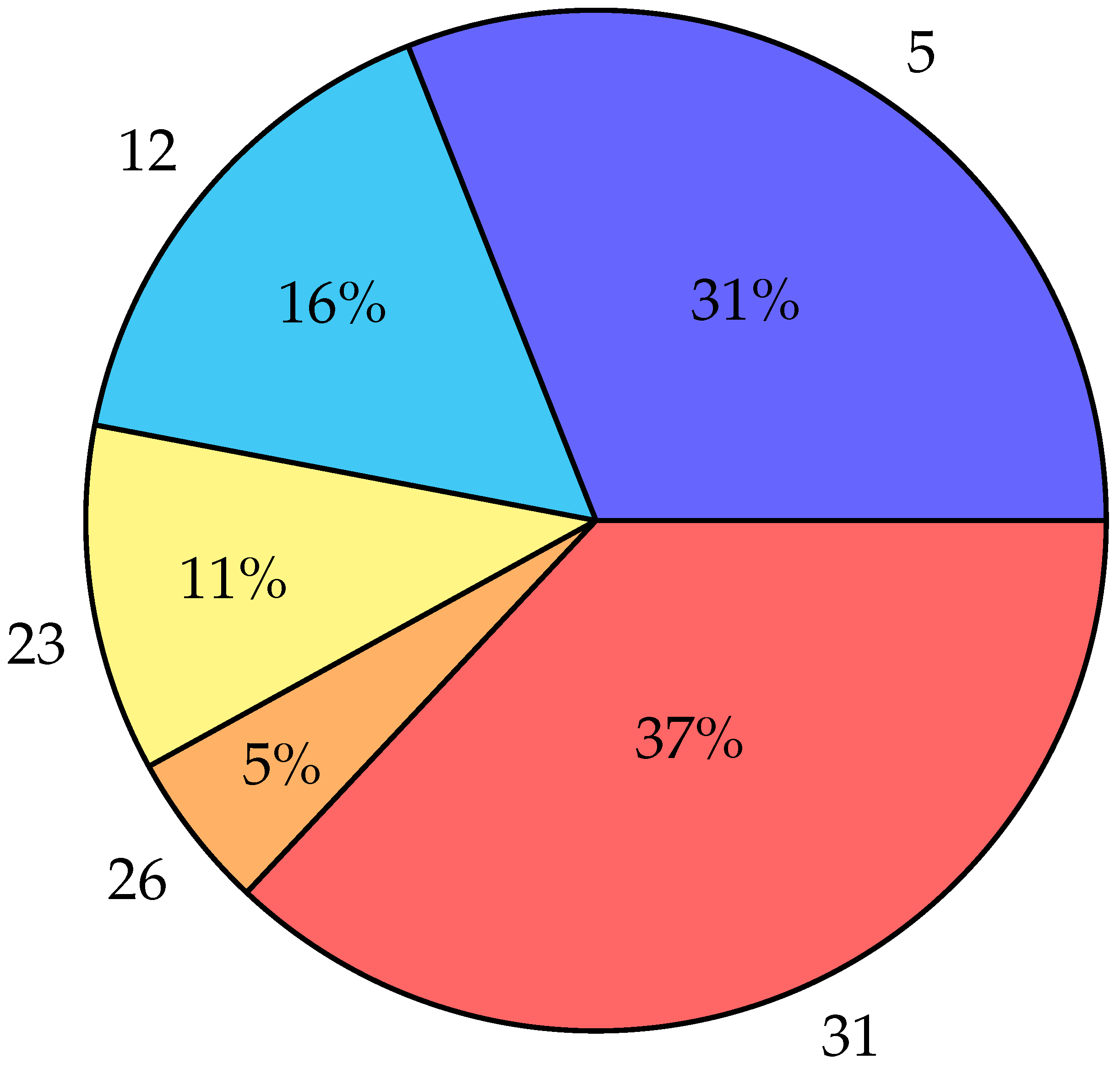
To better understand SBPSO for portfolio optimization, consider the following example. There are 50 assets in the universe. Initially, a set–particle randomly selects a subset of assets, say $\{5,12,23,26,31\}$, from the universe. These assets are then used to create a continuous search space for the inner PSO. Each dimension in the search space of the PSO represents the weight of an asset. Then, the PSO optimizes the asset weights for a fixed duration.

Table 1. Example: Assets and their corresponding weights.

Assets	5	12	23	26	31
Weights	0.31	0.16	0.11	0.05	0.37

contains example results obtained by the weight optimizer.

The combination of the assets and weightings is a candidate portfolio. Continuing with the example, Figure 1 visualizes the portfolio.

Algorithm 3: Set-Based Particle Swarm Optimization for Portfolio Optimization

3.3. Multi-Guide Particle Swarm Optimization

MGPSO is a multi-objective multi-swarm implementation of PSO that uses an archive to share non-dominated solutions between the swarms [27]. Each of the swarms optimizes one of the m objectives for an m-objective optimization problem. The archive, which can be bounded or unbounded, stores non-dominated solutions found by the swarms. MGPSO adds a third guide to the velocity update function, the archive guide, which attracts particles to previously found non-dominated solutions. The archive guide is the winner of a randomly created tournament of archive solutions. The winner is the least crowded solution in the archive. Crowding distance is used to measure how close the solutions are to one another [12]. Alongside the introduction of the archive guide is the archive balance coefficient, i.e., ${\lambda }_i$. The archive balance coefficient is a value from a uniform distribution in the range $[0,1]$ that remains fixed throughout the search. The archive balance coefficient controls the influence of the archive and social guides, where larger values favor the social guide and smaller values favor the archive guide.

The proposal of MGPSO also defines an archive management protocol (summarized in Algorithm 4) according to which a solution is only inserted into the archive if it is not dominated by any existing solution in the archive [27]. Any pre-existing solutions in the archive that are dominated by the newly added solution are removed. In the case that a bounded archive is used and the archive is full, the most crowded solution is removed.

Algorithm 4: Archive Insert Policy

Formally, the velocity update is

$$\begin{array}{cc}\hfill {\mathit{v}}_i(t+1)& =w{\mathit{v}}_i\left(t\right)+c_1{\mathit{r}}_{\mathit{1}}({\mathit{y}}_i\left(t\right)-{\mathit{x}}_i\left(t\right))\hfill \\ \hfill & +{\lambda }_i{c}_2{\mathit{r}}_{\mathit{2}}({\widehat{\mathit{y}}}_i\left(t\right)-{\mathit{x}}_i\left(t\right))\hfill \\ \hfill & +(1-{\lambda }_i)c_3{\mathit{r}}_{\mathit{3}}({\widehat{\mathit{a}}}_i\left(t\right)-{\mathit{x}}_i\left(t\right))\hfill \end{array}$$

(12)

where ${\mathit{r}}_3$ is a vector of random values sampled from a standard uniform distribution in [0, 1]; $c_3$ is the archive acceleration coefficient; ${\widehat{\mathit{a}}}_i$ is the archive guide for particle i. Erwin and Engelbrecht recently proposed an approach for the MGPSO that randomly samples control parameter values from theoretically derived stability conditions, yielding similar performance to that when using tuned parameters [21,27]. Algorithm 5 contains pseudo-code for MGPSO.

Algorithm 5: Multi-Guide Particle Swarm Optimization

3.4. Non-Dominated Sorting Genetic Algorithm II

NSGA-II is a multi-objective GA that ranks and sorts each individual in the population according to its non-domination level [12]. Furthermore, the crowding distance is used to break ties between individuals with the same rank. The use of the crowding distance maintains a diverse population and helps the algorithm explore the search space.

The algorithm uses a single population, $P_t$, of a fixed size, n. At each iteration, a new candidate population, $C_t$, is created by performing crossover (simulated binary crossover) and mutation (polynomial mutation) operations on $P_t$. The two populations are combined to create $Q_t$. $Q_t$ is then sorted by Pareto dominance. Non-dominated individuals are assigned a rank of one and are separated from the population. Individuals that are non-dominated in the remaining population are assigned a rank of two and are separated from the population. This process repeats until all individuals in the population have been assigned a rank. The result is a population separated into multiple fronts, where each front exhibits more Pareto-optimality than the last.

The population, $P_{t+1}$, for the next generation is created by selecting individuals from the sorted fronts. Elitism is preserved by transferring individuals that ranked first into the next generation. If the number of individuals in the first front is greater than n, then the least crowded n individuals (determined by the crowding distance) are selected. If the number of individuals in the first front is less than n, then the least crowded individuals from the second front are selected, and then those from the third front, and so on, until there are n individuals in $P_{t+1}$.

Algorithm 6: Non-Dominated Sorting Genetic Algorithm II

3.5. Strength Pareto Evolutionary Algorithm 2

SPEA2 uses an archive, $A_t$, to ensure that elitism is maintained across generations. SPEA2 also uses a fine-grained fitness assignment. The fitness of an individual takes into account the number of individuals it dominates, the number of solutions it is dominated by, and its density in relation to other individuals.

Like NSGA-II, SPEA2 uses a single population, $P_t$, of a fixed size, n. However, $P_t$ is created by performing crossover (simulated binary crossover) and mutation (polynomial mutation) operations on $A_t$. Individuals in $A_t$ and $P_t$ are assigned strength values. The strength value $S_i$ of individual i is the number of individuals that i dominates. Each individual also has what is referred to as a raw fitness value, $R_i$. $R_i$ is calculated as the summation of the strength values of the individuals that dominate i. Then, to account for the scenario where many, if not all, of the individuals are non-dominated, a density estimator is also added to the fitness calculation. The distance between individual i and every other individual in $R_t$ is calculated and sorted in increasing order. The k-th individual in the sorted list is referred to as ${\alpha }_i^k$. The density of individual i is calculated as

$$D\left(i\right)=\frac{1}{{\alpha }_i^k+2}$$

(13)

Finally, the fitness of individual i is calculated using:

$$F_i=R_i+D_i$$

(14)

All individuals with $F_i\le 1$ are copied over into the archive for the next generation. If the number of individuals in the archive is not enough, the remaining individuals in $Q_t$ are sorted based on $F_i$ in increasing order. The best individuals are selected from the sorted list until the archive is full. When there are too many good-quality individuals, i.e., individuals with $F_i\le 1$, to be inserted into the archive, the individual that has the minimum distance to another individual is removed. This process is repeated until there are n individuals. In the case where there are several individuals with the same minimum distance, then the distances of those individuals to the second, third, etc. closest individuals are considered until the tie is broken.

Algorithm 7: Strength Pareto Evolutionary Algorithm 2

4. Multi-Objective Set-Based Portfolio Optimization Algorithm

This section proposes a multi-objective set-based algorithm for multi-objective portfolio optimization. Elements from MGPSO are incorporated into SBPSO to enable SBPSO to solve multiple objectives simultaneously. The proposed approach, referred to as MGSBPSO, uses multiple swarms, where each swarm optimizes one of the objectives in the asset space. Thus, there is a swarm for selecting assets that minimize risk and a swarm for selecting assets that maximize profit. As for MGPSO, non-dominated solutions found by the swarms are stored in an archive (initially empty) of a fixed size. The archive management process described in Section 3.3 is also used in the MGSBPSO. However, the crowding distance of the non-dominated solutions in the archive is calculated with respect to their objective function values instead of their set-based positions because the set-based positions lack distance in the traditional sense. Non-dominated solutions are selected from the archive using tournament selection and are used to guide the particles to non-dominated regions of the search space. Like the archive management strategy, the crowding distance of the non-dominated solutions in the tournament is calculated with respect to their objective function values. Furthermore, the successful modifications identified by Erwin and Engelbrecht are also included in the MGSBPSO, namely, the removal of zero-weighted assets, the immediate calculation of the objective function for single-asset portfolios, the decision to allow the weight optimizer to execute until it converges, only allowing assets to be removed via the weight determination stage, and the exploration balance coefficient for improved convergence behavior. Taking these improvements, as well as the archive guide, into account, the velocity equation is

$$\begin{array}{cc}\hfill V_i(t+1)=& {\lambda }_c\left(t\right)r_1\otimes (Y_i\left(t\right)\ominus X_i\left(t\right))\hfill \\ \hfill & \oplus {\lambda }_i{\lambda }_c\left(t\right)r_2\otimes ({\widehat{Y}}_i\left(t\right)\ominus X_i\left(t\right))\hfill \\ \hfill & \oplus (1-{\lambda }_i){\lambda }_c{r}_3\otimes ({\widehat{A}}_i\left(t\right)\ominus X_i\left(t\right))\hfill \\ \hfill & \oplus (1-{\lambda }_c\left(t\right))r_4\otimes A_i\left(t\right)\hfill \end{array}$$

(15)

where $r_1$, $r_2$, $r_3$, and $r_4$ are random values, each sampled from a standard uniform distribution in the range [0, 1]; ${\lambda }_c$ is the linearly increasing exploration balance coefficient; $X_i$ is the position of particle i; $Y_i$ is the best position found by particle i; ${\widehat{Y}}_i$ is the best position within particle i’s neighborhood; ${\widehat{A}}_i$ is the archive guide for particle i; the influence of the archive guide is controlled by the archive coefficient ${\lambda }_i$; ${\widehat{A}}_i$ is shorthand for $U\setminus (X\left(t\right)\cup Y\left(t\right)\cup \widehat{Y}\left(t\right))$, where U is the set universe, and ⊗ and ⊕ are the set-based operators defined in Section 3.2.

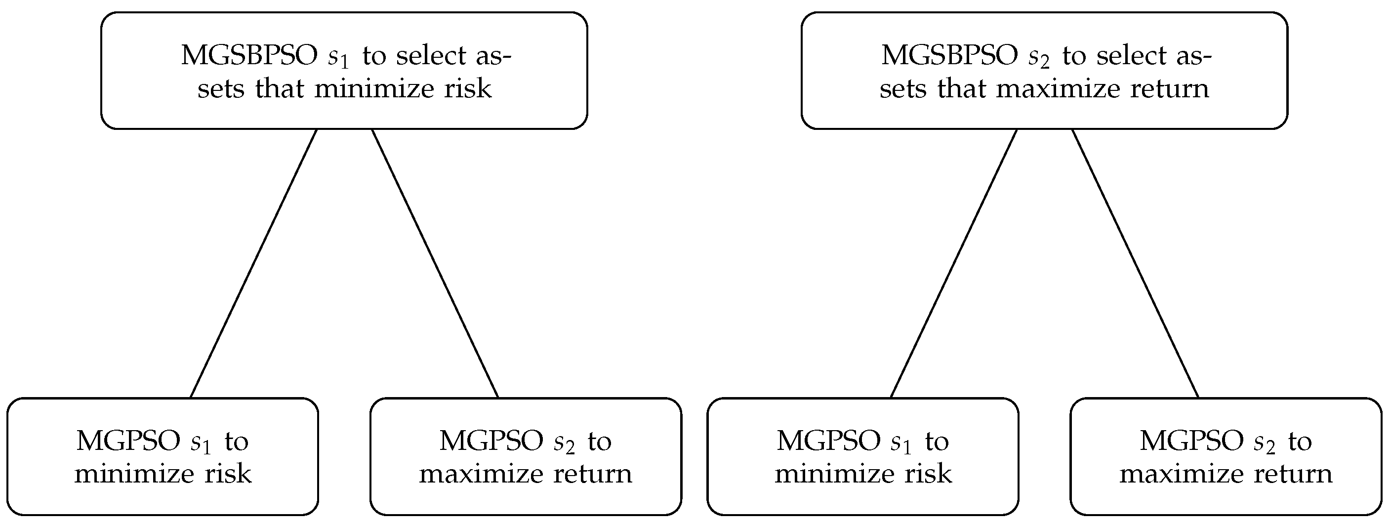
For the purpose of weight determination, MGPSO with the newly proposed tuning-free approach is used. Hence, asset weight determination is also a multi-objective optimization task. For each set–particle, an MGPSO is instantiated to optimize the corresponding asset weights with regard to risk and return. Figure 2 illustrates the overall structure of the swarms in MGSBPSO and their objective.

Each MGPSO in Figure 2 has its own archive. Specifically, the MGPSO for MGSBPSO $s_1$ has its own archive and the MGPSO for MGSBPSO $s_2$ has its own archive. There is also a global archive, the MGSBPSO archive, which is used to store non-dominated solutions found by either MGPSO. An MGPSO terminates when no non-dominated solutions are added to their archives over three iterations. The non-dominated solutions in the archive of an MGPSO are then inserted into the global archive along with the corresponding set position. Lastly, the best objective function value of the non-dominated solutions in an MGPSO archive is assigned to the corresponding set–particle with regard to the objective of the swarm that the set–particle is in. For example, if the set–particle is in the swarm for minimizing risk, then the best risk value of the non-dominated solutions in the MGPSO archive is used. Algorithm 8 presents the pseudocode for the multi-objective weight optimization process and how the MGPSO archives interact with the global archive. The pseudocode for MGSBPSO is given in Algorithm 9.

The proposed MGSBPSO is expected to perform similarly to the MGPSO for multi-objective portfolio optimization, since MGSBPSO makes use of MGPSO for asset weight optimization. It is also expected that the reduction in dimensionality by MGSBPSO will result in higher-quality solutions than those of MGPSO for larger portfolio problems.

Algorithm 8: Multi-Objective Weight Determination for Set-Based Portfolio Optimization

Algorithm 9: Multi-Guide Set-Based Particle Swarm Optimization

5. Empirical Process

This section details the empirical process used to assess the performance of the proposed MGSBPSO. The performance of MGSBPSO is compared with that of MGPSO (using the tuning-free approach), NSGA-II, and SPEA2, where the solution representation is a fixed-length vector of floats. SBPSO is also included to determine if the algorithms perform on par or better.

Section 5.1 describes the implementation of the algorithms. The benchmark problems are discussed in Section 5.2. Section 5.3 describes the constraint-handling technique. The performance measures used are listed in Section 5.4, and Section 5.5 presents the control parameter tuning process used.

5.1. Implementation of Algorithms

SBPSO, MGPSO, and MGSBPSO were implemented by using the Computational Intelligence library (https://github.com/ciren/cilib, accessed on 12 March 2022), and NSGA-II and SPEA2 were implemented by using the JMetal framework [28].

5.2. Benchmark Problems

The benchmark problems in the OR Library (http://people.brunel.ac.uk/mastjjb/jeb/orlib/portinfo.html, accessed on 12 March 2022), which are summarized in

Table 2. Summary of the OR Library datasets for portfolio optimization.

Stock Market	Region	Number of Assets
Hang Seng	Hong Kong	31
DAX 100	Germany	85
FTSE 100	UK	89
S&P 100	USA	98
Nikkei 225	Japan	225

, were used to evaluate the performance of the algorithms. The benchmark problems are based on weekly price data from March 1992 to September 1997—specifically, the mean and standard deviation of the return of each asset and the correlation values for all possible pairs of assets. Furthermore, the OR Library provides a POF that contains 2000 solutions for each benchmark problem. Each solution is a pair of risk and return values.

MGPSO, MGSBPSO, NSGA-II, and SPEA2 were tasked with minimizing (Equation (4)) and maximizing the return (Equation (5)) for each benchmark problem. The algorithms used a population size of 50. In the case of MGPSO and MGSBPSO, 25 particles were allocated to each swarm. SPEA2, MGPSO, and MGSBPSO used a bounded archive of 50 solutions. The final population or archive (in the case of SPEA2, MGPSO, and MGSBPSO) was considered as the obtained POF. SBPSO, which was included in the analysis as a baseline algorithm, optimized Equation (3) for 50 evenly spaced $\lambda$ values. Thus, a POF of 50 non-dominated solutions was produced.

5.3. Constraint Handling

To satisfy Equation (7), any negative asset weights in a candidate solution were treated as zero. Candidate solutions were normalized to satisfy Equation (6). For example, the position $(2.34,-3.12,0.95,1.84,5.33)$ violates both constraints. Using the described constraint-handling technique, the position then becomes $(0.22,0.0,0.09,0.18,0.51)$.

5.4. Performance Measures

Results for each benchmark were collected over 30 independent runs, where each run lasted 5000 iterations (or 250,000 objective function evaluations). After each independent run, the generational distance (GD), inverted generational distance (IGD), and hypervolume (HV) scores were calculated for each algorithm. GD, IGD, and HV are Pareto-optimality measures used to assess the quality of the obtained POFs and are further explained in Appendix B. The mean and standard deviation of these scores (over the 30 independent runs) were tabulated. One-tailed Mann–Whitney U tests with a level of significance of $95\%$ were used to test for any meaningful statistically significant differences between two algorithms. The results of the statistical significance tests were used to rank the algorithms. If an algorithm was statistically significantly better than another algorithm, this was considered a win. Conversely, if an algorithm was statistically significantly worse than another algorithm, this was considered a loss. If there were no statistically significant differences in performance between an algorithm and another algorithm, this was considered a draw. A rank was assigned to each algorithm based on the number of wins.

5.5. Control Parameter Tuning

The control parameters of NSGA-II and SPEA2 were optimized for each benchmark problem so that the algorithms could be compared fairly. To do so, parameter sets were generated using sequences of Sobol pseudo-random numbers that spanned the parameter space of each algorithm [29]. The parameter spaces for NSGA-II and SPEA2 were the same. The crossover probability (${\rho }_c$) and mutation probability (${\rho }_m$) were generated in the range [0.00, 1.00], and the crossover distribution index (${\iota }_c$) and mutation distribution index (${\iota }_c$) were generated in the range [1, 50]. For NSGA-II and SPEA2, 128 parameter sets were evaluated. The parameter sets were then ranked according to their GD, IGD, and HV scores. The best overall parameter set for each benchmark was selected.

Table 3. Optimal control parameter values for the non-dominated sorting genetic Algorithm 2.

Problem	${\mathit{\rho }}_{\mathit{c}}$	${\mathit{\iota }}_{\mathit{c}}$	${\mathit{\rho }}_{\mathit{m}}$	${\mathit{\iota }}_{\mathit{m}}$
Hang Seng	0.3984	1.0	0.8203	46.0
DAX 100	0.4843	41.0	0.5468	44.0
FTSE 100	0.3437	35.0	0.5937	32.0
S&P 100	0.3437	35.0	0.5937	32.0
Nikkei 225	0.4531	17.0	0.8906	42.0

and

Table 4. Optimal control parameter values for the strength pareto evolutionary Algorithm 2.

Problem	${\mathit{\rho }}_{\mathit{c}}$	${\mathit{\iota }}_{\mathit{c}}$	${\mathit{\rho }}_{\mathit{m}}$	${\mathit{\iota }}_{\mathit{m}}$
Hang Seng	0.5859	4.0	0.2578	5.0
DAX 100	0.0078	33.0	0.5234	19.0
FTSE 100	0.4843	41.0	0.546	44.0
S&P 100	0.4843	41.0	0.546	44.0
Nikkei 225	0.4531	17.0	0.890	42.0

list the optimal control parameter values for NSGA-II and SPEA2, respectively.

SBPSO and MGSBPSO did not require control parameter tuning because these algorithms used an exploration balance coefficient. MGPSO used the tuning-free approach. Likewise, the MGPSO weight optimizer for MGSBPSO also used the tuning-free approach. The PSO weight optimizer for SBPSO used the recommended parameters (w = 0.729844 and $c_1$ = $c_2$ = 1.496180 [30]) due to the variability of set–particles and the problems created.

6. Results

This section discusses the results of SBPSO, MGPSO, NSGA-II, SPEA2, and MGSBPSO for each benchmark problem. Section 6.1 examines the Hang Seng results. The DAX 100 and FTSE 100 results are discussed in Section 6.2 and Section 6.3, respectively. Section 6.4 discusses the S&P 100 results, and the Nikkei 225 results are discussed in Section 6.5.

6.1. Hang Seng

Table 5. Hang Seng results for each performance measure.

		R	$\overline{\mathit{\sigma }}$	GD	IGD	HV
SBPSO	$\overline{x}$	0.007607	0.001897	0.000218	0.000212	0.781949
	$\sigma$	0.000003	0.000000	0.000045	0.000002	0.026784
MGPSO	$\overline{x}$	0.007261	0.001967	0.000723	0.000218	1.192743
	$\sigma$	0.000705	0.000407	0.000262	0.000025	0.002658
NSGA-II	$\overline{x}$	0.007859	0.002171	0.000824	0.000200	1.195125
	$\sigma$	0.000103	0.000063	0.000064	0.000006	0.000737
SPEA2	$\overline{x}$	0.007395	0.001921	0.000659	0.000173	1.194271
	$\sigma$	0.000099	0.000046	0.000042	0.000003	0.000345
MGSBPSO	$\overline{x}$	0.007382	0.001814	0.000761	0.000252	1.190891
	$\sigma$	0.000552	0.000326	0.000077	0.000029	0.001930

shows that for the Hang Seng benchmark problem (the smallest benchmark problem), all of the algorithms performed similarly. SBPSO found solutions that were close to POF and diverse. Its multi-objective adaptation obtained a slightly higher GD score, but so did all of the multi-objective algorithms. On average, NSGA-II obtained portfolios with more return, but also more risk. The proposed MGSBPSO had the lowest average risk value, while MGPSO had a higher average risk value and worse return.

Table 6. Hang Seng rankings for each performance measure.

		GD	IGD	HV	Overall
SBPSO	Wins	4	1	0	5
	Losses	0	2	4	6
	Draws	0	1	0	1
	Difference	4	−1	−4	−1
	Rank	1	3	5	4
MGPSO	Wins	2	1	2	5
	Losses	1	2	2	5
	Draws	1	1	0	2
	Difference	1	−1	0	0
	Rank	2	3	3	3
NSGA−II	Wins	0	3	4	7
	Losses	4	1	0	5
	Draws	0	0	0	0
	Difference	−4	2	4	2
	Rank	4	2	1	2
SPEA2	Wins	2	4	3	9
	Losses	1	0	1	2
	Draws	1	0	0	1
	Difference	1	4	2	7
	Rank	2	1	2	1
MGSBPSO	Wins	1	0	1	2
	Losses	3	4	3	10
	Draws	0	0	0	0
	Difference	−2	−4	−2	−8
	Rank	3	4	4	5

shows that SPEA2 was the highest-ranked algorithm, while MGSBPSO ranked last. However, the differences between the values obtained by the algorithms are small. Furthermore, Figure 3 shows that all algorithms were able to approximate the true POF.

6.2. DAX 100

The second benchmark problem included 54 more assets than the previous benchmark problem—a notable increase. The single-objective SBPSO performed well, with the lowest average risk value and second highest average return value (refer to

Table 7. DAX 100 results for each performance measure.

		R	$\overline{\mathit{\sigma }}$	GD	IGD	HV
SBPSO	$\overline{x}$	0.007607	0.001897	0.000218	0.000212	0.781949
	$\sigma$	0.000003	0.000000	0.000045	0.000002	0.026784
MGPSO	$\overline{x}$	0.007261	0.001967	0.000723	0.000218	1.192743
	$\sigma$	0.000705	0.000407	0.000262	0.000025	0.002658
NSGA-II	$\overline{x}$	0.007859	0.002171	0.000824	0.000200	1.195125
	$\sigma$	0.000103	0.000063	0.000064	0.000006	0.000737
SPEA2	$\overline{x}$	0.007395	0.001921	0.000659	0.000173	1.194271
	$\sigma$	0.000099	0.000046	0.000042	0.000003	0.000345
MGSBPSO	$\overline{x}$	0.007382	0.001814	0.000761	0.000252	1.190891
	$\sigma$	0.000552	0.000326	0.000077	0.000029	0.001930

. MGSBPSO also performed well, with average values close to those of SPEA2. The standard deviations of the results for SPEA2 were smaller than those of MGSBPSO, which could explain the large difference in rankings in

Table 8. DAX 100 rankings for each performance measure.

		GD	IGD	HV	Overall
SBPSO	Wins	4	1	0	5
	Losses	0	2	4	6
	Draws	0	1	0	1
	Difference	4	−1	−4	−1
	Rank	1	3	5	4
MGPSO	Wins	2	1	2	5
	Losses	1	2	2	5
	Draws	1	1	0	2
	Difference	1	−1	0	0
	Rank	2	3	3	3
NSGA−II	Wins	0	3	4	7
	Losses	4	1	0	5
	Draws	0	0	0	0
	Difference	−4	2	4	2
	Rank	4	2	1	2
SPEA2	Wins	2	4	3	9
	Losses	1	0	1	2
	Draws	1	0	0	1
	Difference	1	4	2	7
	Rank	2	1	2	1
MGSBPSO	Wins	1	0	1	2
	Losses	3	4	3	10
	Draws	0	0	0	0
	Difference	−2	−4	−2	−8
	Rank	3	4	4	5

. SPEA2 ranked first, while MGSBPSO ranked last. NSGA-II ranked second, MGPSO ranked third, and SBPSO ranked fourth. However, Figure 4d,e show that NSGA-II and SPEA2 (respectively) were only able to approximate a part of the true POF shown in Figure 4a. The PSO algorithms were able to approximate the true POF well, particularly SBPSO and MGSBPSO.

6.3. FTSE 100

FTSE 100 is a similar-sized benchmark problem to DAX 100; however, the outcomes of the results obtained by the algorithms differ. For example,

Table 9. FTSE 100 results for each performance measure.

		R	$\overline{\mathit{\sigma }}$	GD	IGD	HV
SBPSO	$\overline{x}$	0.006683	0.000785	0.000247	0.000235	0.741994
	$\sigma$	0.000007	0.000001	0.000038	0.000007	0.049170
MGPSO	$\overline{x}$	0.005239	0.000570	0.001111	0.000258	1.189333
	$\sigma$	0.000508	0.000097	0.000606	0.000127	0.003496
NSGA-II	$\overline{x}$	0.004446	0.000282	0.000469	0.000548	1.180821
	$\sigma$	0.000130	0.000014	0.000047	0.000037	0.001294
SPEA2	$\overline{x}$	0.004403	0.000287	0.000506	0.000469	1.181466
	$\sigma$	0.000127	0.000015	0.000055	0.000050	0.001235
MGSBPSO	$\overline{x}$	0.005079	0.000438	0.001003	0.000241	1.186224
	$\sigma$	0.000249	0.000048	0.000076	0.000026	0.001914

shows that SBPSO, MGPSO, and MGSBPSO (which had previously obtained more risk-averse solutions) obtained, on average, solutions that were more profitable and risky than those of NSGA-II and SPEA2. Likewise,

Table 10. FTSE 100 rankings for each performance measure.

		GD	IGD	HV	Overall
SBPSO	Wins	4	2	0	6
	Losses	0	1	4	5
	Draws	0	1	0	1
	Difference	4	1	−4	1
	Rank	1	2	5	2
MGPSO	Wins	1	4	4	9
	Losses	3	0	0	3
	Draws	0	0	0	0
	Difference	−2	4	4	6
	Rank	4	1	1	1
NSGA−II	Wins	3	0	1	4
	Losses	1	4	3	8
	Draws	0	0	0	0
	Difference	2	−4	−2	−4
	Rank	2	4	4	5
SPEA2	Wins	2	1	2	5
	Losses	2	3	2	7
	Draws	0	0	0	0
	Difference	0	−2	0	−2
	Rank	3	3	3	4
MGSBPSO	Wins	0	2	3	5
	Losses	4	1	1	6
	Draws	0	1	0	1
	Difference	−4	1	2	−1
	Rank	5	2	2	3

shows that SBPSO, MGPSO, and MGSBPSO ranked higher than NSGA-II and SPEA2. Figure 5 shows that SBPSO and MGSBPSO were able to approximate the true POF better than the other algorithms. NSGA-II and SPEA2 partially approximated (as indicated by the shorter lines) and were unable to find a range of non-dominated solutions. MGPSO, on the other hand, found a variety of non-dominated solutions, but as seen with the multiple arcs branching out, not all independent runs were able to approximate the true POF.

6.4. S&P 100

Table 11. S&P 100 results for each performance measure.

		R	$\overline{\mathit{\sigma }}$	GD	IGD	HV
SBPSO	$\overline{x}$	0.007716	0.001248	0.000275	0.000247	0.875057
	$\sigma$	0.000006	0.000001	0.000044	0.000003	0.044175
MGPSO	$\overline{x}$	0.004993	0.000579	0.001344	0.000276	1.195282
	$\sigma$	0.000359	0.000150	0.000235	0.000037	0.001887
NSGA-II	$\overline{x}$	0.004521	0.000254	0.000626	0.000594	1.188502
	$\sigma$	0.000130	0.000015	0.000036	0.000033	0.001069
SPEA2	$\overline{x}$	0.004352	0.000243	0.000580	0.000541	1.187435
	$\sigma$	0.000170	0.000019	0.000045	0.000052	0.001274
MGSBPSO	$\overline{x}$	0.004819	0.000388	0.001263	0.000330	1.190151
	$\sigma$	0.000195	0.000053	0.000099	0.000038	0.001808

shows that, for the S&P 100 benchmark problem, NSGA-II, SPEA2, MGPSO, and MGSBPSO obtained similar averages for return and risk. SBPSO, on the other hand, obtained solutions with more return and risk. NSGA-II and SPEA2 were the most risk-averse algorithms with lower return values. The low return and risk values of NSGA-II and SPEA2 make sense, as Figure 6 shows that these algorithms were (only) able to approximate the lower part of the true POF. SBPSO ranked first, as shown in

Table 12. S&P 100 rankings for each performance measure.

		GD	IGD	HV	Overall
SBPSO	Wins	4	4	0	8
	Losses	0	0	4	4
	Draws	0	0	0	0
	Difference	4	4	−4	4
	Rank	1	1	5	1
MGPSO	Wins	0	3	4	7
	Losses	3	1	0	4
	Draws	1	0	0	1
	Difference	−3	2	4	3
	Rank	4	2	1	2
NSGA−II	Wins	2	0	2	4
	Losses	2	4	2	8
	Draws	0	0	0	0
	Difference	0	−4	0	−4
	Rank	3	5	3	5
SPEA2	Wins	3	1	1	5
	Losses	1	3	3	7
	Draws	0	0	0	0
	Difference	2	−2	−2	−2
	Rank	2	4	4	4
MGSBPSO	Wins	0	2	3	5
	Losses	3	2	1	6
	Draws	1	0	0	1
	Difference	−3	0	2	−1
	Rank	4	3	2	3

, but with the worst HV ranking. MGPSO and MGSBPSO ranked second and third, respectively, while the multi-objective GAs, SPEA2, and NSGA-II ranked fourth and last, respectively. Lastly, Figure 6c shows that MGSBPSO was able to approximate the upper part of the true POF the best out of the multi-objective algorithms. MGSBPSO reached the stopping condition in 110 s, and MGPSO reached it in 160 s. SPEA2 and NSGA-II, on the other hand, were faster and reached the stopping condition in approximately 80 s. Note that the difference in time could be due to the different programming libraries used to implement the algorithms (see Section 5.1).

6.5. Nikkei 225

The last and largest benchmark problem to discuss is Nikkei 225. Nikkei 225 contained 255 assets, which was more than twice that of the last benchmark problem and a significant increase in dimensionality.

Table 13. Nikkei 225 results for each performance measure.

		R	$\overline{\mathit{\sigma }}$	GD	IGD	HV
SBPSO	$\overline{x}$	0.003310	0.000794	0.000260	0.000223	0.916014
	$\sigma$	0.000007	0.000001	0.000060	0.000005	0.047097
MGPSO	$\overline{x}$	0.002193	0.000650	0.001631	0.000294	1.190877
	$\sigma$	0.000338	0.000122	0.000393	0.000051	0.003675
NSGA-II	$\overline{x}$	0.002146	0.000444	0.000579	0.000226	1.190051
	$\sigma$	0.000069	0.000010	0.000047	0.000015	0.001352
SPEA2	$\overline{x}$	0.002002	0.000445	0.000562	0.000161	1.193376
	$\sigma$	0.000052	0.000010	0.000047	0.000006	0.000557
MGSBPSO	$\overline{x}$	0.002437	0.000633	0.001242	0.000242	1.191968
	$\sigma$	0.000272	0.000113	0.000114	0.000030	0.003169

shows that all of the algorithms obtained similar values, with the exceptions (as in the previous results) of MGPSO and MGSBPSO, which obtained higher GD values, and SBPSO, which obtained a lower HV value. The rankings for this problem are given in

Table 14. Nikkei 225 rankings for each performance measure.

		GD	IGD	HV	Overall
SBPSO	Wins	4	2	0	6
	Losses	0	1	4	5
	Draws	0	1	0	1
	Difference	4	1	−4	1
	Rank	1	2	5	2
MGPSO	Wins	0	0	1	1
	Losses	4	4	1	9
	Draws	0	0	2	2
	Difference	−4	−4	0	−8
	Rank	4	4	3	4
NSGA−II	Wins	2	2	1	5
	Losses	1	1	2	4
	Draws	1	1	1	3
	Difference	1	1	−1	1
	Rank	2	2	4	2
SPEA2	Wins	2	4	4	10
	Losses	1	0	0	1
	Draws	1	0	0	1
	Difference	1	4	4	9
	Rank	2	1	1	1
MGSBPSO	Wins	1	1	2	4
	Losses	3	3	1	7
	Draws	0	0	1	1
	Difference	−2	−2	1	−3
	Rank	3	3	2	3

and show that SPEA2 was the best-performing algorithm overall. SBPSO and NSGA-II tied for second place, while MGSBPSO and MGPSO ranked third and last, respectively. Once again, visual analysis of the obtained POFs (shown in Figure 7) provides useful context for the results. Figure 7d,e show that NSGA-II and SPEA2, respectively, were able to approximate the lower part of the true POF, with SPEA2 performing slightly better than NSGA-II. The POF obtained by MGPSO is wide and scattered, which makes sense as to why MGPSO ranked last. On the other hand, SBPSO and MGSBPSO were able to approximate the true POF better than all of the other algorithms. There were some breaks in the POF obtained by SBPSO, while the POF obtained by MGSBPSO was fully connected, but slightly thicker. Nonetheless, both SBPSO and MGSBPSO performed better than the other algorithms in approximating the true POF. MGSBPSO, NSGA-II, and SPEA2 reached the stopping condition in approximately 400 s, while MGPSO took 650 s to reach the stopping condition.

7. Conclusions

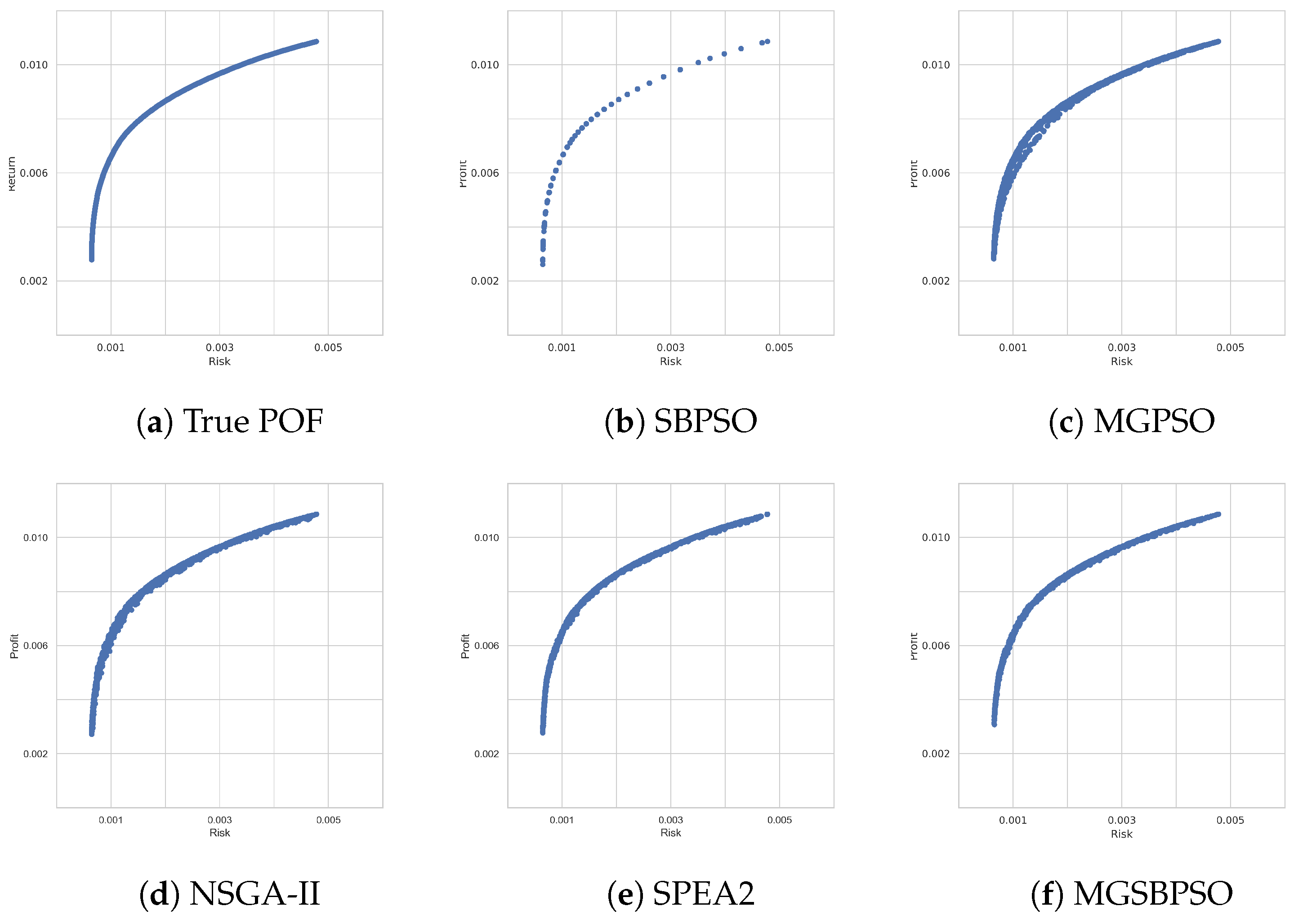
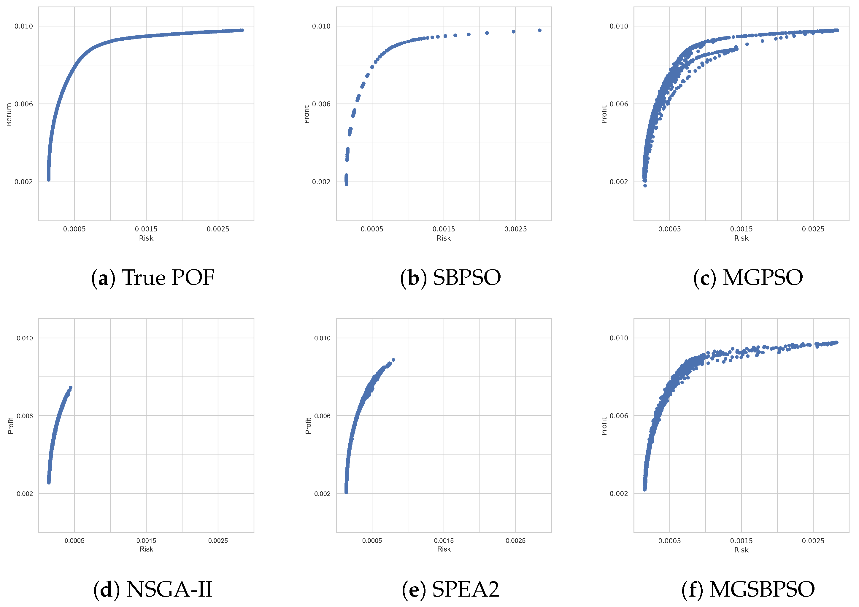
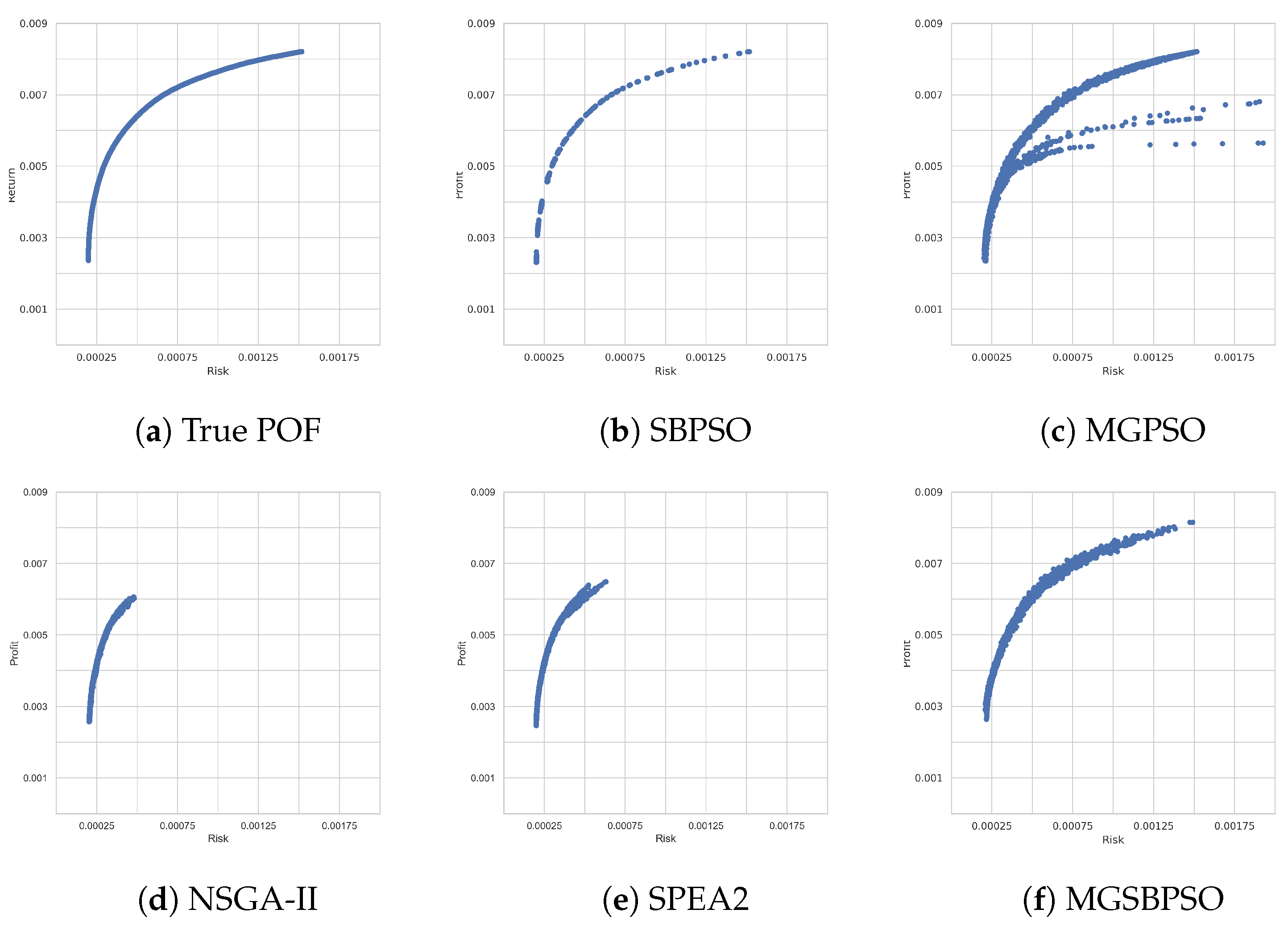
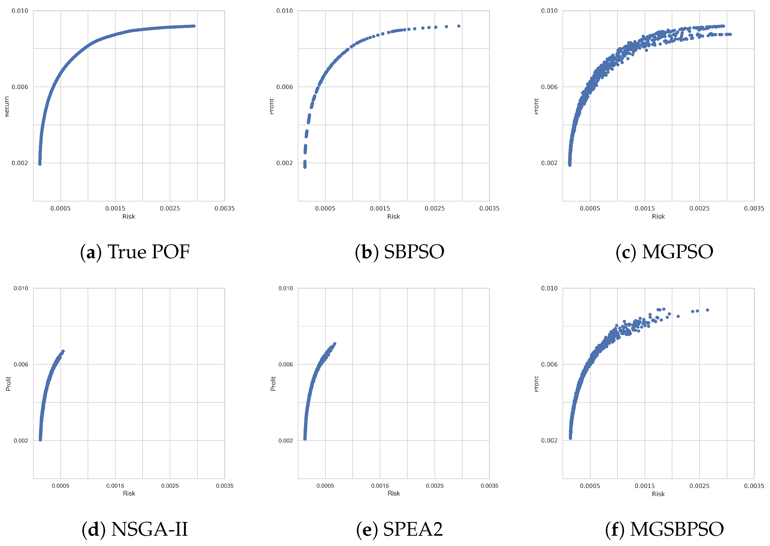
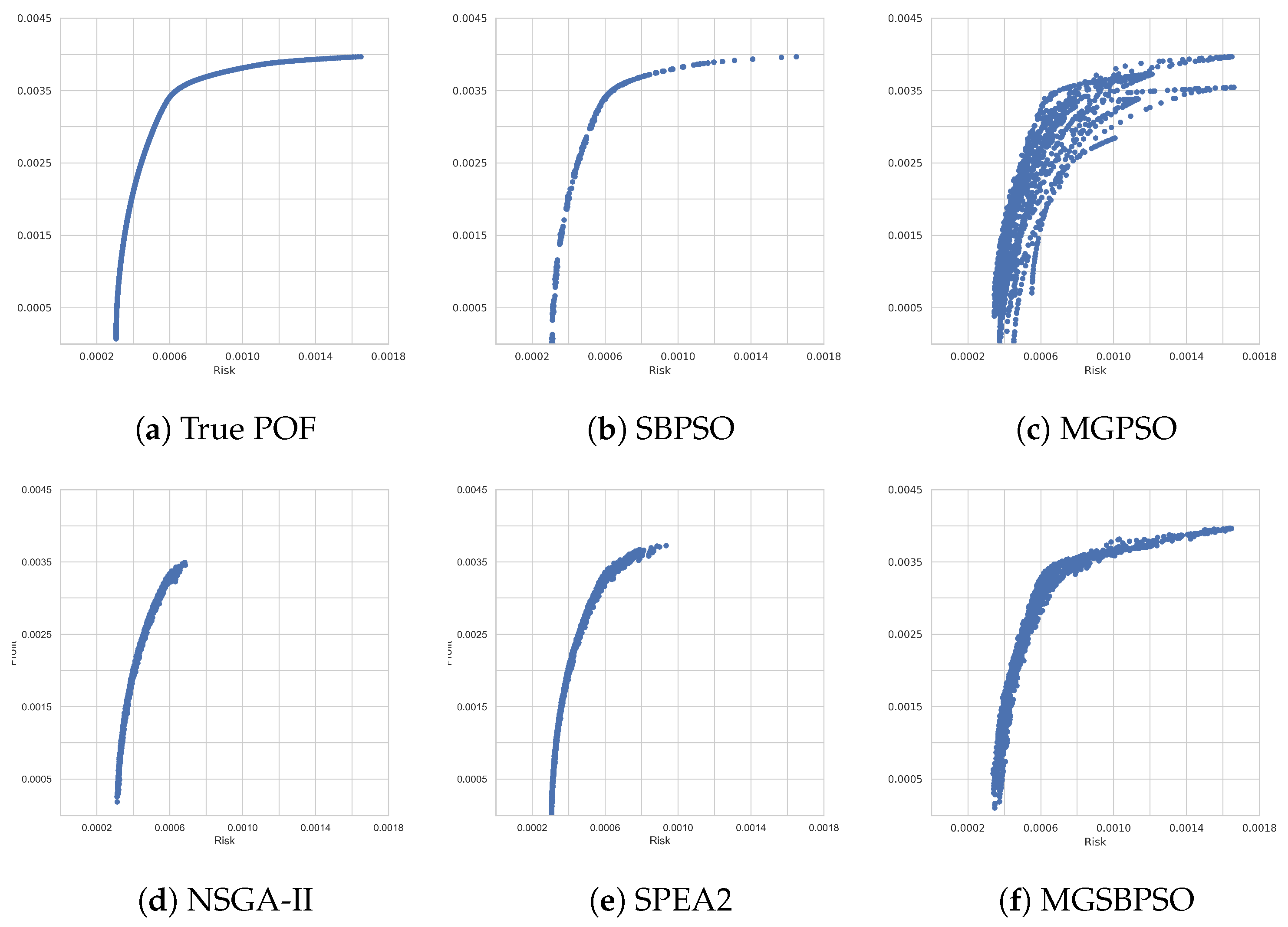
This paper proposed the multi-guide set-based particle swarm optimization (MGSBPSO) algorithm, a multi-objective adaptation of the set-based particle swarm optimization (SBPSO) algorithm that incorporates elements from multi-guide particle swarm optimization (MGPSO). MGSBPSO uses two set-based swarms, where the first selects assets that minimize risk, and the second swarm selects assets that maximize return. For the purpose of optimizing the asset weights, MGPSO, which samples’ control parameter values that satisfy theoretically derived stability criteria, was used. The performance of MGSBPSO was compared with that of MGPSO, NSGA-II, SPEA2, and the single-objective SBPSO across five portfolio optimization benchmark problems.

The results showed that all algorithms, in general, were able to approximate the true Pareto-optimal front (POF). NSGA-II and SPEA2 generally ranked quite high in comparison with the other algorithms. However, visual analysis of the POF obtained by NSGA-II and SPEA2 shows that these algorithms were only able to approximate part of the true POF. SBPSO, MGPSO, and MGSBPSO were able to approximate the full true POF for each benchmark problem, with the exception of MGPSO, for the last (and largest) benchmark problem. MGPSO, as well as MGSBPSO and SBPSO, did not scale to the largest portfolio problem, which redefined portfolio optimization as a set-based optimization problem. SBPSO optimized the mean-variance portfolio model of Equation (3) for a given risk–return tradeoff value. By optimizing for multiple tradeoff values, SBPSO obtained a variety of solutions with differing risk and return characteristics. Thus, an advantage of MGSBPSO over its single-objective counterpart is that MGSBPSO does not require multiple runs to obtain a diverse set of optimal solutions, as risk (minimized) and return (maximized) are optimized independently of each other. It should also be noted that MGPSO without control parameter tuning performed similar to or better than NSGA-II and SPEA2 with tuned parameters.

Overall, the results show that the benefits of redefining the portfolio optimization problem as a set-based problem are also applicable to multi-objective portfolio optimization.

8. Future Work

Future work should focus on improving the performance of MGSBPSO for portfolio optimization. A part of this work could investigate the effects of different swarm sizes on the performance of MGSBPSO. Another opportunity for future work is to investigate the performance of MGSBPSO for traditional multi-objective combinatorial problems, such as multi-objective knapsack problems.

References

1. Cura, T. A rapidly converging artificial bee colony algorithm for portfolio optimization. Knowl.-Based Syst. 2021, 233, 107505. [Google Scholar] [CrossRef]
2. Akbay, M.A.; Kalayci, C.B.; Polat, O. A parallel variable neighborhood search algorithm with quadratic programming for cardinality constrained portfolio optimization. Knowl.-Based Syst. 2020, 198, 105944. [Google Scholar] [CrossRef]
3. Kalayci, C.B.; Ertenlice, O.; Akbay, M.A. A comprehensive review of deterministic models and applications for mean-variance portfolio optimization. Expert Syst. Appl. 2019, 125, 345–368. [Google Scholar] [CrossRef]
4. Woodside-Oriakhi, M.; Lucas, C.; Beasley, J. Heuristic algorithms for the cardinality constrained efficient frontier. Eur. J. Oper. Res. 2011, 213, 538–550. [Google Scholar] [CrossRef]
5. Moral-Escudero, R.; Ruiz-Torrubiano, R.; Suarez, A. Selection of optimal investment portfolios with cardinality constraints. In Proceedings of the IEEE International Conference on Evolutionary Computation, Vancouver, BC, Canada, 16–21 July 2006; pp. 2382–2388. [Google Scholar]
6. Ruiz-Torrubiano, R.; Suarez, A. Use of heuristic rules in evolutionary methods for the selection of optimal investment portfolios. In Proceedings of the IEEE Congress on Evolutionary Computation, Singapore, 25–28 September 2007; pp. 212–219. [Google Scholar]
7. Ruiz-Torrubiano, R.; Suarez, A. Hybrid approaches and dimensionality reduction for portfolio selection with cardinality constraints. IEEE Comput. Intell. Mag. 2010, 5, 92–107. [Google Scholar] [CrossRef]
8. Ruiz-Torrubiano, R.; Suarez, A. A memetic algorithm for cardinality-constrained portfolio optimization with transaction costs. Appl. Soft Comput. 2015, 36, 125–142. [Google Scholar] [CrossRef] [Green Version]
9. Streichert, F.; Tanaka-Yamawaki, M. The effect of local search on the constrained portfolio selection problem. In Proceedings of the IEEE International Conference on Evolutionary Computation, Vancouver, BC, Canada, 16–21 July 2006; pp. 2368–2374. [Google Scholar]
10. Erwin, K.; Engelbrecht, A.P. Improved set-based particle swarm optimization for portfolio optimization. In Proceedings of the IEEE Swarm Intelligence Symposium, Canberra, ACT, Australia, 1–4 December 2020; pp. 1573–1580. [Google Scholar]
11. Scheepers, C. Multi-Guide Particle Swarm Optimization A Multi-Swarm Multi-Objective Particle Swarm Optimizer. Ph.D. Thesis, Department of Computer Science, University of Pretoria, Pretoria, South Africa, 2018. [Google Scholar]
12. Deb, K.; Pratap, A.; Agarwal, S.; Meyarivan, T. A fast and elitist multi–objective genetic algorithm: NSGA-II. IEEE Trans. Evol. Comput. 2002, 6, 182–197. [Google Scholar] [CrossRef] [Green Version]
13. Zitzler, E.; Laumanns, M.; Thiele, L. SPEA2: Improving the strength Pareto evolutionary algorithm. TIK-Rep. 2001, 103, 1–22. [Google Scholar]
14. Skolpadungket, P.; Dahal, K.; Harnpornchai, N. Portfolio optimization using multi-objective genetic algorithms. In Proceedings of the IEEE Congress on Evolutionary Computation, Singapore, 25–28 September 2007; pp. 516–523. [Google Scholar]
15. Chiam, S.C.; Al Mamun, A.; Low, Y.L. A realistic approach to evolutionary multi–objective portfolio optimization. In Proceedings of the IEEE Congress on Evolutionary Computation, Singapore, 25–28 September 2007; pp. 204–211. [Google Scholar]
16. Chiam, S.C.; Tan, K.C.; Al Mamum, A. Evolutionary multi-objective portfolio optimization in practical context. Int. J. Autom. Comput. 2008, 5, 67–80. [Google Scholar] [CrossRef]
17. Anagnostopoulos, K.P.; Mamanis, G. Multiobjective evolutionary algorithms for complex portfolio optimization problems. Comput. Manag. Sci. 2009, 8, 259–279. [Google Scholar] [CrossRef]
18. Anagnostopoulos, K.P.; Mamanis, G. A portfolio optimization model with three objectives and discrete variables. Comput. Oper. Res. 2010, 37, 1285–1297. [Google Scholar] [CrossRef]
19. Branke, J.; Scheckenbach, B.; Stein, M.; Deb, K.; Schmeck, H. Portfolio optimization with an envelope-based multi-objective evolutionary algorithm. Eur. J. Oper. Res. 2009, 199, 684–693. [Google Scholar] [CrossRef]
20. Anagnostopoulos, K.P.; Mamanis, G. The mean variance cardinality constrained portfolio optimization problem: An experimental evaluation of five multi–objective evolutionary algorithms. Expert Syst. Appl. 2011, 38, 14208–14217. [Google Scholar] [CrossRef]
21. Erwin, K.; Engelbrecht, A.P. A tuning free approach to multi-guide particle swarm optimization. In Proceedings of the 2021 IEEE Symposium Series on Computational Intelligence (SSCI), Orlando, FL, USA, 5–7 December 2021. [Google Scholar]
22. Engelbrecht, A. Computational Intelligence—An Introduction, 2nd ed.; Wiley: Hoboken, NJ, USA, 2007. [Google Scholar]
23. Eberhart, R.; Kennedy, J. A new optimizer using particle swarm theory. In Proceedings of the Sixth International Symposium on Micro Machine and Human Science, Nagoya, Japan, 4–6 October 1995; pp. 39–43. [Google Scholar]
24. Shi, Y.; Eberhart, R. A modified particle swarm optimizer. In Proceedings of the IEEE International Conference on Evolutionary Computation, Anchorage, AK, USA, 4–9 May 1998; pp. 69–73. [Google Scholar]
25. Langeveld, J.; Engelbrecht, A.P.P. Set-based particle swarm optimization applied to the multidimensional knapsack problem. Swarm Intell. 2012, 6, 297–342. [Google Scholar] [CrossRef] [Green Version]
26. Erwin, K.; Engelbrecht, A.P. Set-Based particle swarm optimization for portfolio optimization. In Proceedings of the International Conference on Swarm Intelligence, ANTS Conference, Barcelona, Spain, 26–28 October 2020; pp. 333–339. [Google Scholar]
27. Scheepers, C.; Cleghorn, C.; Engelbrecht, A.P. Multi-guide particle swarm optimization for multi-objective optimization: Empirical and stability analysis. Swarm Intell. 2019, 13, 245–276. [Google Scholar] [CrossRef]
28. Nebro, A.J.; Durillo, J.J.; Vergne, M. Redesigning the jMetal Multi-Objective Optimization Framework. In Proceedings of the Companion Publication of the 2015 Annual Conference on Genetic and Evolutionary Computation, GECCO Companion ’15, Madrid, Spain, 11–15 July 2015; Association for Computing Machinery: New York, NY, USA, 2015; pp. 1093–1100. [Google Scholar] [CrossRef]
29. Franken, N. Visual exploration of algorithm parameter space. In Proceedings of the IEEE Congress on Evolutionary Computation, Trondheim, Norway, 18–21 May 2009; pp. 389–398. [Google Scholar]
30. Cleghorn, C.W.; Engelbrecht, A.P. Particle swarm convergence: An empirical investigation. In Proceedings of the IEEE Congress of Evolutionary Computation, Beijing, China, 6–11 July 2014; Volume 1, pp. 2524–2530. [Google Scholar]
31. Van Veldhuizen, D.A.; Lamont, G.B. On measuring multi–objective evolutionary algorithm performance. In Proceedings of the Congress on Evolutionary Computation, La Jolla, CA, USA, 16–19 July 2000; Volume 1, pp. 204–211. [Google Scholar]
32. Tsai, S.J.; Sun, T.Y.; Liu, C.C.; Hsieh, S.T.; Wu, W.C.; Chiu, S.Y. An improved multi-objective particle swarm optimizer for multi-objective problems. Expert Syst. Appl. 2010, 37, 5872–5886. [Google Scholar] [CrossRef]
33. Zitzler, E.; Thiele, L.; Laumanns, M.; Fonseca, C.M.; da Fonseca, V.G. Performance assessment of multi–objective optimizers: An analysis and review. IEEE Trans. Evol. Comput. 2003, 7, 117–132. [Google Scholar] [CrossRef]
Figure 1. Example: Assets and their corresponding weights as pie chart.
Algorithms 16 00062 g001
Figure 2. MGSBPSO structure.
Algorithms 16 00062 g002
Figure 3. Obtained Pareto-optimal fronts for Hang Seng.
Algorithms 16 00062 g003
Figure 4. Obtained Pareto-optimal fronts for DAX 100.
Algorithms 16 00062 g004
Figure 5. Pareto-optimal fronts obtained for FTSE 100.
Algorithms 16 00062 g005
Figure 6. Pareto-optimal fronts obtained for S&P 100.
Algorithms 16 00062 g006
Figure 7. Pareto-optimal obtained fronts for Nikkei 225.
Algorithms 16 00062 g007