Abstract
In this paper, we present a novel unsupervised feature selection method termed robust matrix factorization with robust adaptive structure learning (RMFRASL), which can select discriminative features from a large amount of multimedia data to improve the performance of classification and clustering tasks. RMFRASL integrates three models (robust matrix factorization, adaptive structure learning, and structure regularization) into a unified framework. More specifically, a robust matrix factorization-based feature selection (RMFFS) model is proposed by introducing an indicator matrix to measure the importance of features, and the L21-norm is adopted as a metric to enhance the robustness of feature selection. Furthermore, a robust adaptive structure learning (RASL) model based on the self-representation capability of the samples is designed to discover the geometric structure relationships of original data. Lastly, a structure regularization (SR) term is designed on the learned graph structure, which constrains the selected features to preserve the structure information in the selected feature space. To solve the objective function of our proposed RMFRASL, an iterative optimization algorithm is proposed. By comparing our method with some state-of-the-art unsupervised feature selection approaches on several publicly available databases, the advantage of the proposed RMFRASL is demonstrated.
1. Introduction
In recent years, with the rapid development of the Internet and the popularization of mobile devices, it has become more and more convenient to analyze, search, transmit, and process large amounts of data, which can also promote the development of society and the sharing of resources. However, with the continuous advancement of information technology, mobile Internet data are becoming enormous [1], inevitably increasing the amount of data needing to be processed in real life. Although these high-dimensional data can bring us helpful information, they also cause problems such as data redundancy and noisy data [2,3,4]. Dimensionality reduction technology can not only avoid the “curse of dimensionality” by removing redundant and irrelevant features, but also reduce the time-consuming nature of data processing and the storage space of data [5]. Therefore, it is widely used to process large quantities of Internet mobile data [6]. The most commonly used dimensionality reduction techniques are feature extraction and feature selection. Feature extraction projects the original high-dimensional data into a low-dimensional subspace [7,8,9]. Unlike feature extraction, feature selection selects an optimal subset from the original feature set. Since feature selection can preserve the semantics of original features, it is more explicable and physical; thus, it has been widely used in many fields, e.g., intrusion detection of industrial Internet [10], simulated attack of Internet of things [11], and computer vision [12].
According to the presence or absence of labels, feature selection methods can be divided into supervised, semi-supervised, and unsupervised methods. Among them, unsupervised feature selection is a significant challenge research because few labeled data are available in real life [13]. Unsupervised feature selection can be divided into three categories: (1) filtering methods, (2) wrapping methods, and (3) embedding-based methods. The filtering method involves performing feature selection on the original dataset in advance and then training a learner. In other words, the procedure of feature selection is independent of the learner training [14]. The wrapping method continuously selects feature subsets from the initial dataset and trains the learner until the optimal feature subset is selected [15,16]. Embedding automatically performs feature selection during the learning process. Compared with the filtering and wrapping methods, embedded methods can significantly reduce the computational cost and achieve good results [17,18].
He et al. [19] proposed an unsupervised feature selection method named Laplacian score (LS), which selects optimal feature subsets to preserve the local manifold structure of the original data. However, the LS method ignores the correlation between features. In order to overcome this disadvantage, Liu et al. [20] proposed an unsupervised feature selection method with robust neighborhood embedding (RNEFS). RNEFS adopts the local linear embedding (LLE) algorithm to compute the feature weight matrix. Then, the L1-norm-based reconstructing error was utilized to suppress the influence of noise and outliers. Subsequently, Wang et al. [21] proposed an efficient soft label feature selection (SLFS) method, which first performed soft label learning and then selected features on the basis of the learned soft labels. However, weight matrices of the above methods were defined in advance by considering the similarity of features, which may have affected their performances due to the quality of weight matrices. Therefore, Yuan et al. [22] proposed an adaptive graph convex non-negative matrix analysis method for unsupervised feature selection (CNAFS) which embedded self-expression and pseudo-label information into a joint model. CNAFS can select the most representative features by computing top-ranked features. Shang et al. [23] proposed a non-negative matrix factorization adaptive constraint-based feature selection (NNSAFS) method, which introduced a feature map into matrix factorization to combine manifold learning and feature selection. By combining feature transformation with adaptive constraints, NNSAFS can significantly improve the accuracy of feature selection. However, the above methods take Euclidean distance as the metric. Euclidean distance is sensitive to noise and redundant data, which may cause the performance to be unstable and not robust. To address this issue, Zhao et al. [24] proposed a joint adaptive and discriminative unsupervised feature selection method, which adaptively learns similar graphs while employing irrelevance constraints to enhance the discriminability of the selected features. Zhu et al. [25] proposed a regularized self-representation (RSR) model, which efficiently performs feature selection by using the self-representation ability of features with the L21-norm error to guarantee robustness. Shi et al. [26] proposed a robust spectral learning framework, which utilized graph embedding and spectral regression to deal with noise during unsupervised feature selection. Du et al. [27] proposed a robust unsupervised feature selection based on the matrix factorization (RUFSM) method, which adopted the L21-norm to improve robustness and preserve the local manifold structure, so that an optimal feature subset could be found to retain the manifold structure information. Miao et al. [28] proposed an unsupervised feature selection method named graph-regularized local linear embedding (GRLLE), which combined linear embedding and graph regularization into a unified framework while maintaining local spatial structure. However, the correlation between the selected features was still ignored in the above methods.
This paper proposes an unsupervised feature selection method called robust matrix factorization with robust adaptive structure learning (RMFRASL) to solve the above problems. First, this paper presents a robust matrix factorization-based feature selection model (RMFFS), which introduces a feature indicator matrix into matrix factorization with an L21-norm-based error metric. Next, a robust adaptive structure learning (RASL) model based on self-representation capability is proposed to better describe the local geometry of the samples, which can reduce redundant and noisy features to learn a more discriminative graph structure. Then, to preserve the geometric structure information during the feature selection, a structure regularization (SR) term is constructed. Finally, the above three models are combined into a unified framework and shown in Figure 1. In summary, the main contributions of this paper are as follows:
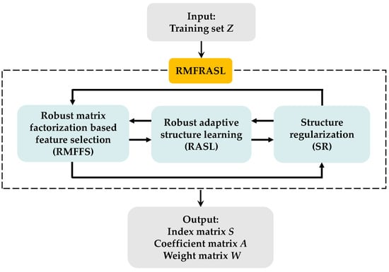
Figure 1.
The structure flowchart of the proposed RMFRASL method.
(1) In order to overcome the shortcoming of existing methods in that they neglect the correlation of features, we introduce an indicator matrix into matrix factorization and design a robust matrix factorization-based feature selection (RMFFS).
(2) To consider the structure information during the process of feature selection, a structure regularization term is integrated into the RMFFS model.
(3) To solve the disadvantages of the existing methods needing to predefine a graph structure, a robust adaptive structure learning model based on the self-representation capability of the sample is proposed, which adopts L21-norm as an error metric rather than L2-norm to reduce the influence of noise or outliers.
(4) To further improve the performance of feature selection methods, an unfiled framework is proposed by combining the process of the feature selection and structure learning.
(5) An iterative optimization algorithm is designed to solve the objective function, and the convergence of the optimization algorithm is verified from mathematical theory and numerical experiments.
This paper is organized as follows: Section 2 briefly reviews the related work. The proposed RMFRASL model is introduced in Section 3. The convergence analysis is provided in Section 4. The experimental results and analysis are provided in Section 5. Section 6 gives the conclusions and future research works.
2. Related Work
2.1. Notations
Assume that is a matrix with the size of n × d to represent high-dimensional original data, where n and d denote the number of data and features, and is a row vector with the size of d to denote the j-th data of Z. L1-norm, L2-norm, and L21-norm of the matrix Z can be defined as follows:
According to the above definitions and matrix correlation operations [29], we can obtain that , where denotes the diagonal matrix whose diagonal elements are . For ease of reading, a description of the commonly used symbols is listed in Table 1.

Table 1.
Description of commonly used symbols.
2.2. Introduction of Indicator Matrix
The indicator matrix is a binary matrix, where denotes a column vector with only one element value equal to 1. To understand the indicator matrix S for feature selection more clearly, we establish an example. First, we assume that the data matrix contains four samples, and that each sample has five features; the data matrix can be described as follows:
Then, supposing that three features are selected (i.e., f1, f4 and f5), we can obtain the selected feature subset as follows:
Meanwhile, the indicator matrix S can be assumed as follows:
Thus, we can obtain
Equation (7) can describe the process of feature selection using the indicator matrix S. Finally, we can also obtain as follows:
3. Robust Matrix Factorization with Robust Adaptive Structure Learning
In this section, a robust matrix factorization with robust adaptive structure learning (RMFRASL) model for unsupervised feature selection is developed to deal with multimedia data collected from Internet of things. Then, an iterative optimization method is designed to solve the objective function of the proposed method. Lastly, a description and the time complexity of the proposed algorithm are provided.
3.1. The Proposed RMFRASL Model
The RMFRASL effectively integrates three models, i.e., robust matrix factorization-based feature selection (RMFFS), robust adaptive structure learning (RASL), and structure regularization (SR), into a unified framework.
3.1.1. RMFFS Model
In order to take the correlation of features into consideration, the self-representation of data or features is widely used for feature representation learning [30]. Therefore, a new feature selection model named robust matrix factorization-based feature selection (RMFFS) is proposed. In the proposed RMFFS model, we first utilize an indicator matrix to find a suitable subset of features for capturing the most critical information to represent the original features approximately. Then, unlike the previous methods, the L21-norm metric is imposed on the reconstruction errors to improve the effectiveness and enhance robustness of feature selection. As a result, the objective function of the RMFFS model is defined as follows:
where is an identity matrix with the size of k, is a coefficient matrix which maps the original features from high-dimensional space into a new low-dimensional space, is defined as a feature weight matrix, and k is the number of selected features. The constraint conditions of and are to force each element of matrix S to be either one or zero and at most a nonzero element in any row or column during the iterative update process. Thus, the matrix S can be considered as an indicator matrix for the selected features under these constraint conditions.
3.1.2. RASL Model
Although the proposed RMFFS model can implement feature selection, it does not sufficiently consider the local structure relationships among original data, which may lead to unsatisfactory performance. Therefore, a robust structure learning method based on the self-representation capability of the original data is proposed, which can learn non-negative representation coefficients to indicate the structural relationships among original data. In order to learn more discriminative non-negative representation coefficients, an error metric function with L21-norm is imposed. Hence, the objective function of RASL is defined as follows:
where denotes the non-negative representation coefficient matrix. The element of matrix W with a larger value means that the correlation between two data is more remarkable.
3.1.3. SR Model
Preserving the structure of selected feature space is very important for feature learning [31]. Thus, a structure regularization (SR) term is designed, which can be defined as follows:
where denotes the selected feature of sample zi, L is a Laplacian matrix defined by [32], and D is a diagonal matrix with elements of .
3.1.4. The Framework of RMFRASL
The three modules (feature selection, robust structure learning, and structure regularization) are integrated into a unified framework to obtain the final objective function of RMFRASL as follows:
where and are tradeoff parameters that adjust the importance of each term in the model.
3.2. Model Optimization
The proposed model has three variables (S, A, and W) to be solved. The objective function of Equation (12) is not a convex optimization problem for all variables [32]. Therefore, we cannot obtain the globally optimal solution for the objective function. In order to solve the above problem, we need to design an iterative optimization algorithm. Specifically, we can optimize one of the variables while fixing the remainder, with alternate iterative updates until the objective function converges.
3.2.1. Fix A and W; Update S
For Equation (12), removing the irrelevant term with S yields the following objective function:
However, the constraint conditions in Equation (13) make it difficult to optimize; hence, we can alleviate the constraint condition to as a penalty term. Thus, Equation (13) is transformed into the following objective function:
where the parameter λ > 0 is used to constrain the orthogonality of vector S.
Let ; according to the above definitions and matrix correlation operations [29], Equation (14) can be simplified to Equation (15) through a series of algebraic operations:
where denotes the diagonal matrix defined as follows:
where ε is a small constant.
To solve Equation (15), a Lagrange multiplier with non-negative constraint is introduced, and the Lagrangian function can be defined as follows:
The partial derivative of Equation (17) with respect to matrix S can be obtained as follows:
Equation (19) can be obtained according to the KKT condition () [33].
The update formula of the matrix S is as follows:
where , , and .
3.2.2. Fix S and W; Update A
For Equation (12), removing the irrelevant term with A yields the following objective function:
Through a series of algebraic formulas [29], Equation (21) can be simplified as
Likewise, the Lagrangian multiplier with a non-negative constraint is introduced to solve Equation (22), and the Lagrangian function can be expressed as follows:
The partial derivative of Equation (23) with respect to A is defined as follows:
As the complementary relaxation of the KKT condition leads to , we can get Equation (25).
According to Equation (25), the update rule of the matrix A is as follows:
3.2.3. Fix S and A; Update W
For Equation (12), the following objective function can be obtained by removing the irrelevant term with W:
where , and .
Through a series of algebraic formulas [29], Equation (27) can be simplified as
where and is a diagonal matrix defined as follows:
To solve Equation (28), a Lagrange multiplier for the non-negative constraint is introduced, and the Lagrangian function is defined as follows:
The partial derivative Equation (30) with respect to W can be shown as follows:
As the complementary relaxation of the KKT condition leads to , we can obtain Equation (32).
The update formula for the matrix W is as follows:
3.3. Algorithm Description
The pseudo code of RMFRASL is listed in Algorithm 1, and a flowchart of the proposed method is shown Figure 2. Moreover, the termination condition of the algorithm is that the change in objective function values between two successive iterations is less than a threshold or has reached the predefined maximum number of iterations in our work.
| Algorithm 1 RMFRASL algorithm |
| Input: The matrix of sample dataset , parameters α > 0, β > 0, λ > 0 1: Initialization: matrices S0, A0, and W0 are initial nonnegative matrices, t = 0 2: Calculate matrices Ut, and Ct according to Equations (16) and (29), 3: Repeat 4: Update St according to Equation (20) 5: Update At according to Equation (26) 6: Update Wt according to Equation (33) 7: Update Ut and Ct according to Equations (16) and (29) 8: Update t = t + 1 9: Until the objective function is convergent. |
| Output: Index matrix S, coefficient matrix A, and weight matrix W |
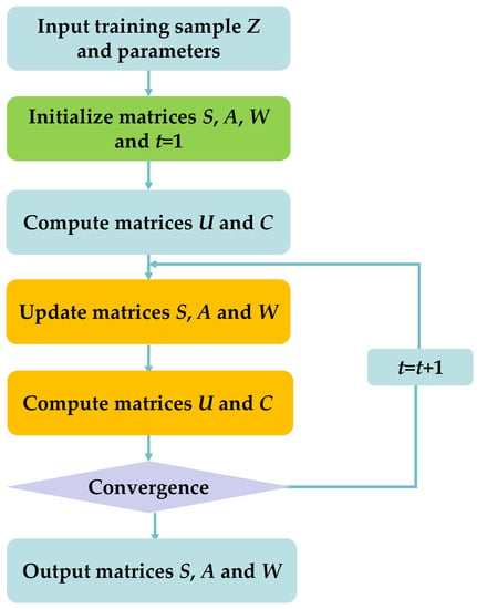
Figure 2.
The flowchart of the proposed RMFRASL method.
3.4. Computational Complexity Analysis
The computational complexity can be calculated in light of the above flowchart of the proposed RMFRASL algorithm. First, the computational complexities of all variables in one iteration are shown in Table 2, where d, n, and k represent the dimensions of the original sample, the number of samples, and the number of selected features, respectively. Since k << d and k << n, we only need to compare the size of d and n. (1) If d > n, S, A, and W need O(nd2), O(kdn), and O(nd2), respectively. Then, the computational complexity of the RMFRASL algorithm is O(t × nd2 ) where t is the number of iterations. (2) If n≥ d, S, A, and W need O(dn2), O(kn2), and O(dn2), respectively. Then, the computational complexity of the RMFRASL algorithm is O(t × dn2). Finally, we can conclude that the computational complexity of the RMFRASL algorithm is O(t × max (dn2, nd2) + dn2).
Table 2.
Computational complexity of each variable.
Meanwhile, the running time of the proposed RMFRASL and other compared feature selection methods was also tested when the number of experimental iterations was set to 10. From the experimental results listed in Table 3, the running time of the proposed method was lower than that of the other compared methods.
Table 3.
Running time (s) of each method on different databases.
4. Convergence Analysis
In order to analyze the convergence of the proposed RMFRASL method, we firstly establish some theorems and definitions below.
Theorem 1.
For variables S, A, and W, the value of Equation (12) is nonincreasing under the update rules of Equations (20), (26) and (33).
We can refer to the convergence analysis of NMF to solve the above theorem. Therefore, some auxiliary functions are introduced below.
Definition 1.
is an auxiliary function ofifandsatisfy the following conditions [35]:
Lemma 1.
Ifis an auxiliary function of, then it is nonincreasing under the following conditions:
Proof.
In order to apply Lemma 1 to prove Theorem 1, we need to find suitable auxiliary functions for the variables S, A, and W. Therefore, the functions, first-order derivatives, and second-order derivatives of the three variables are specified. □
Then, we can obtain the three lemmas described below.
Lemma 2.
The function
is an auxiliary function of .
Lemma 3.
The function
is an auxiliary function of .
Lemma 4.
The function
is an auxiliary function of .
Next, we can prove Lemma 2 using the steps below.
Proof the Lemma 2.
The Taylor series expansion of can be given as follows:
□
We can obtain the following inequalities through a series of calculations of the matrix:
To sum up, we can obtain the inequality
Therefore, we can obtain Equation (54).
Similarly, we can prove Lemma 3 and Lemma 4. Finally, according to Lemma 1, we can obtain the update scheme of variables S, A, and W as follows:
In summary, Theorem 1 is proven.
Next, the convergence of the proposed iterative procedure in Algorithm 1 is proven.
For any nonzero vectors and , the following inequality can be obtained:
More detailed proof of Equation (58) is similar to that in [36].
Theorem 2.
According to the iterative update approach depicted in Algorithm 1, the objective function value in Equation (12) monotonically decreases in each iteration until it converges to the global optimum [36].
Proof.
First, matrices Ut and Ct are denoted as the t-th iteration of matrices U and C. Then, when fixing Ut and Ct, matrices St+1, At+1, and Wt+1 can be updated by solving the following inequality:
□
The above inequality can be changed to
On the basis of the definitions of matrices Ut and Ct, the following inequalities can be obtained:
According to Equation (58), the following inequalities can be obtained:
Combining Equation (61) to Equation (64), the following inequality can be obtained:
From Equation (65), we can clearly see that Equation (12) is monotonically decreasing during iterations and has a lower bound. Therefore, the proposed iterative optimization algorithm will converge. Moreover, numerical experiments verified that the objective function values of our proposed method tend to converge.
5. Experiments and Analysis
In this section, we compare the proposed RMFRASL method with some advanced unsupervised feature selection methods in recent years for classification and clustering tasks, mainly consisting of LSFS [19], RNEFS [20], USFS [21], CNAFS [22], NNSAFS [23], RSR [25], and SPNFSR [34].
5.1. Description of Compared Methods
RNEFS [20] is a robust neighborhood embedding unsupervised feature selection method that employs the locally linear embedding (LLE) to compute the feature weight matrix and minimizes the reconstruction error using the L1-norm. USFS [21] guides feature selection by combining the feature selection matrix with soft labels learned in the low-dimensional subspace. CNAFS [22] combines adaptive graph learning with pseudo-label matrices and constructs two different manifold regularizations with pseudo-label and projection matrices. NNSAFS [23] uses residual terms from sparse regression and introduces feature graphs and maximum entropy theory to construct the manifold structure. RSR [25] uses a linear combination to represent the correlation among each feature. Meanwhile, it also imposes an L21-norm on the loss function and weight matrix to select representative features. SPNFSR [34] constructs a low-rank graph to maintain the global and local structure of data and employs the L21-norm to constrain the representation coefficients for feature selection. The summarization of the methods is shown in Table 4.
Table 4.
The summarization of compared methods in this paper.
5.2. Description of Experimental Data
In this experiment, we performed classification and clustering tasks [37] on five publicly available datasets, including four publicly available face datasets (AR, CMU PIE, Extended YaleB, and ORL) and one object dataset (COIL20). The specific details of the five datasets are shown in Table 5, where Tr and Te represent the number of training samples and testing samples selected from each class.
Table 5.
Details of five databases.
The AR [38] database consists of 4000 images corresponding to face images of 70 males and 56 females. The photos have different facial expressions, lighting conditions, and occlusions. There are 26 images for each object. Some examples of the AR database are shown in Figure 3a.
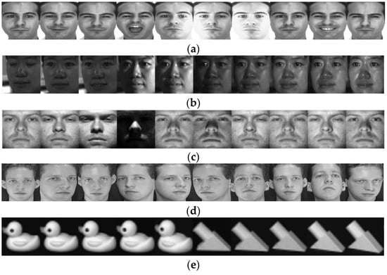
Figure 3.
Selected images from the five databases: (a) AR; (b) CMU PIE; (c) Extended YaleB; (d) ORL; (e) COIL20.
The CMU PIE [39] database consists of 41,368 multi-pose, illumination, and expression face images, including face images with different pose conditions, illumination conditions, and expressions for each object. Some instances of the CMU PIE database are shown in Figure 3b.
The Extended YaleB [40] database consists of 2414 images containing 38 objects with 64 photographs taken for each object, with strict control over pose, lighting, and the shooting angle. Some face images of the Extended YaleB database are shown in Figure 3c.
The ORL [41] dataset consists of 400 face images containing 40 subjects taken at different times of day, under different lighting, and with different facial expressions. Some examples of the ORL dataset are shown in Figure 3d.
The COIL20 [42] dataset contains 1440 images, taken from 20 objects at different angles, with 72 images per object. Some images the COIL20 dataset are shown in Figure 3e.
5.3. Experimental Evaluation
For the classification task, the nearest neighbor classifier (NNC) [43] was employed to classify the selected features of each method, and the classification accuracy rate was used to evaluate the performance, which is defined as
where Ncor and Ntol denote the number of the samples that are accurately classified and the number of all samples for classification, respectively.
For the clustering task, we applied the k-means clustering to cluster the selected features of different methods, and we adopted clustering accuracy (ACC) [44,45,46] to evaluate their performances. The ACC is defined as follows:
where n is total number of the test samples, lk and ck denote the ground truth and the corresponding clustering result of the test sample xk, respectively, and is a function which is defined as follows:
is a mapping function that projects each clustering label ck to its corresponding truth label lk using the Kuhn–Munkres algorithm. Moreover, normalized mutual information (NMI) [46] was also used to test the clustering performance, which is defined as follows:
where U and V denotes two arbitrary variables, H(U) and H(V) are defined as the entropies of U and V, and I(U, V) is defined as the mutual information of variables U and V.
5.4. Experimental Setting
In the experiments of this paper, we randomly selected T sample data from each database as the training sample set and the remaining C sample data as the test samples. All experiments were repeated 10 times, and the average of their classification accuracy was calculated. In order to find the best parameters for the proposed method, a grid search method [47] was used. For the three balance parameters α, β, and λ, the values of α and β were set in the range {0, 0.01, 0.1, 1, 10, 100, 1000, and 10,000}, and λ was set as large as possible (i.e., 100,000) in this work. For the feature dimensions, we set the range from 60 to 560 with intervals of every 100 dimensions.
5.5. Analysis of Experimental Results
5.5.1. Classification Performance Analysis
In the first experiment, we tested the influence of parameter values on the classification performance of the proposed method. First, we analyzed the impact of each balance parameter (i.e., α and β) on the accuracy of the RMFRASL method. From the experimental results shown in Figure 4, we can observe that (1) when the value of parameters is set to 0, the performance of the proposed RMFRASL method is relatively low. Thus, adding these two terms is necessary for feature selection. (2) With the parameter value increasing, the performance of the method also improves, which indicates that introducing the two terms can enhance the discriminatory capability of the selected features. (3) When the performance of the proposed method reaches the optimal value, it decreases or remains stable as the value of the parameter increases. This phenomenon may be due to the parameters being set as larger values such that the importance of the second and third terms of the objective function is overemphasized, while the first term is neglected. As a result, the proposed method is unable to extract the discriminatory features. Then, we evaluated the impact of the number of iterations on the performance of the proposed method. Figure 5 shows the classification accuracy of RMFRASL with different numbers of iterations on five datasets, where the number of iterations was set to {20, 100, 200, 300, 400, and 500}. The experimental results show that the accuracy rate increased with the number of iterations between 20 and 100 and then stabilized or decreased slightly. The best combination of parameters for the classification task is listed in Table 6.
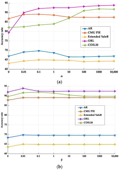
Figure 4.
The classification accuracy rate of different parameter values: (a) parameter α; (b) parameter β.
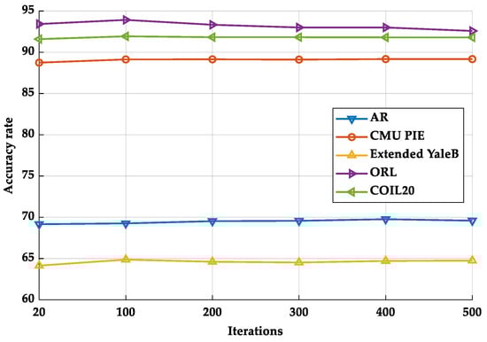
Figure 5.
Accuracy rate of the proposed RMFRASL method on each database with different iteration.
Table 6.
The optimal combination of parameters and dimension on the classification task.
In the second experiment, we compared the performance of different feature selection methods. The classification accuracies of each unsupervised feature selection method on the five databases are given in Table 7. From the experimental results, we can find that, due to the LSFS computing the feature scores without considering the correlation of the selected feature, its performance was the worst. The RNEFS considers the feature self-representation capability; hence, its performance was better than LSFS. The performance of USFS was superior to RNEFS and LSFS since it incorporates soft label learning and constructs the regression relationships between the soft label matrix and features to guides feature selection. CNAFS and NNSAFS combine the geometric structure of the data or features and can select more discriminatory features to obtain slightly higher classification accuracy than RNEFS and USFS. Since RSR and SPNFSR exploit the feature self-representation capability and define the reconstruction error with L21-norm to significantly improve robustness to noise, their performances are better than other compared methods. However, SPNFSR outperforms RSR due to it considering the geometric structure of features. By fully considering the feature self-representation, geometric structure, adaptive graph learning, and robustness together, our proposed RMFRASL achieved the best results among all compared methods. The classification accuracy rate curves of different feature selection methods with different numbers of selected features are shown in Figure 6. First, with the increase in the number of selected features, the classification accuracy rates of all methods improved. Then, the classification accuracy rates of most methods began to stabilize after achieving their best performances.
Table 7.
The best accuracy rate and STD of different algorithms on the five databases.
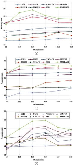
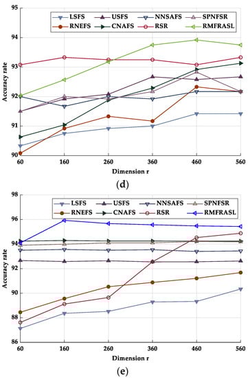
Figure 6.
Accuracy rate of each database in different dimensions: (a) AR; (b) CMU PIE; (c) Extended YaleB; (d) ORL; (e) COIL20.
5.5.2. Clustering Performance Analysis
In this subsection, the k-means method was used for the clustering task. To reduce the randomness of initialization in k-means, we report the mean of 10 experiments. First, the effect of different parameters on the performance of the proposed method was tested. The experimental results of each balance parameter (i.e., α and β) on the clustering of the RMFRASL method are shown in Figure 7. The results show that the influences of the balance parameters on the performance of our method were similar to those for the classification experiments. Then, after setting the optimal parameter settings for RMFRASL in Table 8, the clustering results on ACC and NMI were as shown in Table 9 and Table 10, consistent with the classification experiments.
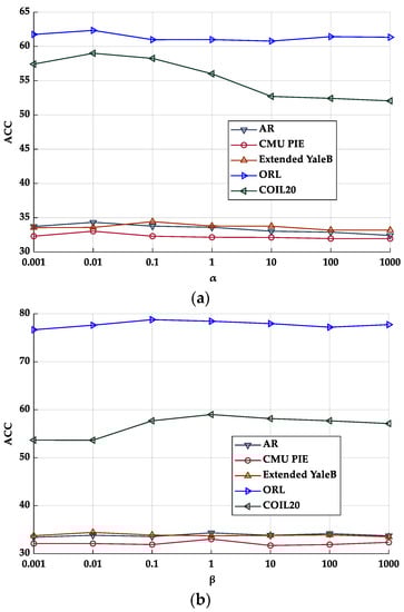
Figure 7.
The clustering accuracy (ACC) of different parameter values: (a) parameter α; (b) parameter β.
Table 8.
The optimal combination of parameters and dimension on the clustering task.
Table 9.
The best ACC% and STD of different algorithms on the five databases.
Table 10.
The best NMI% and STD of different algorithms on the five databases.
5.5.3. Convergence Analysis
In this subsection, we set the parameters to their respective optimal combinations in each of the five databases; then, iterative convergence analysis was performed. Figure 8 shows that RMFRASL achieved convergence with a small number of iterations on each database. Moreover, we provide the number of iterations needed by the compared methods to achieve convergence in Table 11. According to this table, the number of iterations of the proposed RMFRASL method was lower than that of the other methods in most cases.
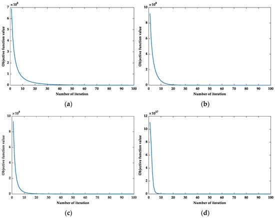
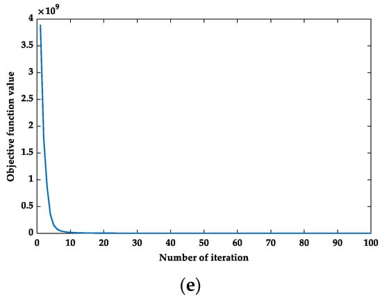
Figure 8.
The convergence of the RMFRASL algorithm: (a) AR; (b) CMU PIE; (c) Extended YaleB; (d) ORL; (e) COIL20.
Table 11.
The number of iterations of different algorithms on the five databases.
6. Discussion and Future Work
Feature selection is an effective dimensionality reduction technique, and previous methods did not consider the performance of adaptive graph learning and robustness simultaneously. To solve the above problems, this paper proposed a robust adaptive structure learning-based matrix factorization (RMFRASL) method, which integrates feature selection and adaptive graph learning into a unified framework. A large number of experiments showed that RMFRASL could achieve better performance than previous methods. Deep learning and transfer learning show excellent promise in feature learning tasks. In future work, it may be possible to introduce deep learning and transfer learning schemes into feature selection to develop a more efficient feature selection method.
Author Contributions
Data curation, S.L., L.H., P.L. and Z.L.; formal analysis, S.L., P.L. and Z.L.; methodology, S.L., L.H. and Y.Y.; resources, S.L. and Z.L.; supervision, L.H. and Y.Y.; writing—original draft, S.L., L.H. and J.W.; writing—review and editing, Y.Y. and J.W. All authors have read and agreed to the published version of the manuscript.
Funding
This research was funded by National Natural Science Foundation of China (Nos. 62062040, 62006174, and 61967010), the Outstanding Youth Project of Jiangxi Natural Science Foundation (No. 20212ACB212003), the Jiangxi Province Key Subject Academic and Technical Leader Funding Project (No. 20212BCJ23017), and the Fund of Jilin Provincial Science and Technology Department (No. 20210101187JC).
Data Availability Statement
The data were derived from public domain resources.
Conflicts of Interest
The authors declare no conflict of interest.
References
- Cheng, X.; Fang, L.; Hong, X.; Yang, L. Exploiting mobile big data: Sources, features, and applications. IEEE Netw. 2017, 31, 72–79. [Google Scholar] [CrossRef]
- Cheng, X.; Fang, L.; Yang, L.; Cui, S. Mobile big data: The fuel for data-driven wireless. IEEE Internet Things J. 2017, 4, 1489–1516. [Google Scholar] [CrossRef]
- Lv, Z.; Lou, R.; Li, J.; Singh, A.K.; Song, H. Big data analytics for 6G-enabled massive internet of things. IEEE Internet Things J. 2021, 8, 5350–5359. [Google Scholar] [CrossRef]
- Tang, C.; Zheng, X.; Liu, X.; Zhang, W.; Zhang, J.; Xiong, J.; Wang, L. Cross-view locality preserved diversity and consensus learning for multi-view unsupervised feature selection. IEEE Trans. Knowl. Data Eng. 2021, 34, 4705–4716. [Google Scholar] [CrossRef]
- Jin, J.; Xiao, R.; Daly, I.; Miao, Y.; Wang, X.; Cichocki, A. Internal feature selection method of CSP based on L1-norm and Dempster-Shafer theory. IEEE Trans. Neural Netw. Learn. Syst. 2020, 32, 4814–4825. [Google Scholar] [CrossRef] [PubMed]
- Zhu, F.; Ning, Y.; Chen, X.; Zhao, Y.; Gang, Y. On removing potential redundant constraints for SVOR learning. Appl. Soft Comput. 2021, 102, 106941. [Google Scholar] [CrossRef]
- Li, Z.; Nie, F.; Bian, J.; Wu, D.; Li, X. Sparse pca via L2,p-norm regularization for unsupervised feature selection. IEEE Trans. Pattern Anal. Mach. Intell. 2021, 1–8. [Google Scholar] [CrossRef] [PubMed]
- Luo, F.; Zou, Z.; Liu, J.; Lin, Z. Dimensionality reduction and classification of hyperspectral image via multistructure unified discriminative embedding. IEEE Trans. Geosci. Remote Sens. 2021, 60, 1–16. [Google Scholar] [CrossRef]
- Lee, D.D.; Seung, H.S. Learning the parts of objects by non-negative matrix factorization. Nature 1999, 401, 788–791. [Google Scholar] [CrossRef]
- Awotunde, J.B.; Chakraborty, C.; Adeniyi, A.E. Intrusion detection in industrial internet of things network-based on deep learning model with rule-based feature selection. Wirel. Commun. Mob. Comput. 2021, 2021, 7154587. [Google Scholar] [CrossRef]
- Aminanto, M.E.; Choi, R.; Tanuwidjaja, H.C.; Yoo, P.D.; Kim, K. Deep abstraction and weighted feature selection for Wi-Fi impersonation detection. IEEE Trans. Inf. Secur. 2017, 13, 621–636. [Google Scholar] [CrossRef]
- Zhang, F.; Li, W.; Feng, Z. Data driven feature selection for machine learning algorithms in computer vision. IEEE Internet Things J. 2018, 5, 4262–4272. [Google Scholar] [CrossRef]
- Qi, M.; Wang, T.; Liu, F.; Zhang, B.; Wang, J.; Yi, Y. Unsupervised feature selection by regularized matrix factorization. Neurocomputing 2018, 273, 593–610. [Google Scholar] [CrossRef]
- Zhai, Y.; Ong, Y.S.; Tsang, I.W. The emerging “big dimensionality”. IEEE Comput. Intell. Mag. 2014, 9, 14–26. [Google Scholar] [CrossRef]
- Bermejo, P.; Gámez, J.A.; Puerta, J.M. Speeding up incremental wrapper feature subset selection with Naive Bayes classifier. Knowl. -Based Syst. 2014, 55, 140–147. [Google Scholar] [CrossRef]
- Cheng, L.; Wang, Y.; Liu, X.; Li, B. Outlier detection ensemble with embedded feature selection. In Proceedings of the AAAI Conference on Artificial Intelligence, New York, NY, USA, 7–12 February 2020; Volume 34, pp. 3503–3512. [Google Scholar]
- Lu, Q.; Li, X.; Dong, Y. Structure preserving unsupervised feature selection. Neurocomputing 2018, 301, 36–45. [Google Scholar] [CrossRef]
- Li, X.; Zhang, H.; Zhang, R.; Liu, Y.; Nie, F. Generalized uncorrelated regression with adaptive graph for unsupervised feature selection. IEEE Trans. Neural Netw. Learn. Syst. 2018, 30, 1587–1595. [Google Scholar] [CrossRef]
- He, X.; Cai, D.; Niyogi, P. Laplacian score for feature selection. Adv. Neural Inf. Process. Syst. 2005, 18, 1–8. [Google Scholar]
- Liu, Y.; Ye, D.; Li, W.; Wang, H.; Gao, Y. Robust neighborhood embedding for unsupervised feature selection. Knowl.-Based Syst. 2020, 193, 105462. [Google Scholar] [CrossRef]
- Wang, F.; Zhu, L.; Li, J.; Chen, H.; Zhang, H. Unsupervised soft-label feature selection. Knowl.-Based Syst. 2021, 219, 106847. [Google Scholar] [CrossRef]
- Yuan, A.; You, M.; He, D.; Li, X. Convex non-negative matrix factorization with adaptive graph for unsupervised feature selection. IEEE Trans. Cybern. 2020, 52, 5522–5534. [Google Scholar] [CrossRef] [PubMed]
- Shang, R.; Zhang, W.; Lu, M.; Jiao, L.; Li, Y. Feature selection based on non-negative spectral feature learning and adaptive rank constraint. Knowl.-Based Syst. 2022, 236, 107749. [Google Scholar] [CrossRef]
- Zhao, H.; Li, Q.; Wang, Z.; Nie, F. Joint Adaptive Graph Learning and Discriminative Analysis for Unsupervised Feature Selection. Cogn. Comput. 2022, 14, 1211–1221. [Google Scholar] [CrossRef]
- Zhu, P.; Zuo, W.; Zhang, L.; Hu, Q.; Shiu, S.C. Unsupervised feature selection by regularized self-representation. Pattern Recognit. 2015, 48, 438–446. [Google Scholar] [CrossRef]
- Shi, L.; Du, L.; Shen, Y.D. Robust spectral learning for unsupervised feature selection. In Proceedings of the 2014 IEEE International Conference on Data Mining, Shenzhen, China, 14–17 December 2014; pp. 977–982. [Google Scholar]
- Du, S.; Ma, Y.; Li, S.; Ma, Y. Robust unsupervised feature selection via matrix factorization. Neurocomputing 2017, 241, 115–127. [Google Scholar] [CrossRef]
- Miao, J.; Yang, T.; Sun, L.; Fei, X.; Niu, L.; Shi, Y. Graph regularized locally linear embedding for unsupervised feature selection. Pattern Recognit. 2022, 122, 108299. [Google Scholar] [CrossRef]
- Hou, C.; Nie, F.; Li, X.; Yi, D.; Wu, Y. Joint embedding learning and sparse regression: A framework for unsupervised feature selection. IEEE Trans. Cybern. 2013, 44, 793–804. [Google Scholar]
- Wang, S.; Pedrycz, W.; Zhu, Q.; Zhu, W. Subspace learning for unsupervised feature selection via matrix factorization. Pattern Recognit. 2015, 48, 10–19. [Google Scholar] [CrossRef]
- Zhu, F.; Gao, J.; Yang, J.; Ye, N. Neighborhood linear discriminant analysis. Pattern Recognit. 2022, 123, 108422. [Google Scholar] [CrossRef]
- Cai, D.; He, X.; Han, J.; Huang, T.S. Graph regularized nonnegative matrix factorization for data representation. IEEE Trans. Pattern Anal. Mach. Intell. 2010, 33, 1548–1560. [Google Scholar]
- Dreves, A.; Facchinei, F.; Kanzow, C.; Sagratella, S. On the solution of the KKT conditions of generalized Nash equilibrium problems. SIAM J. Optim. 2011, 21, 1082–1108. [Google Scholar] [CrossRef]
- Zhou, W.; Wu, C.; Yi, Y.; Luo, G. Structure preserving non-negative feature self-representation for unsupervised feature selection. IEEE Access 2017, 5, 8792–8803. [Google Scholar] [CrossRef]
- Yi, Y.; Zhou, W.; Liu, Q.; Luo, G.; Wang, J.; Fang, Y.; Zheng, C. Ordinal preserving matrix factorization for unsupervised feature selection. Signal Process. Image Commun. 2018, 67, 118–131. [Google Scholar] [CrossRef]
- Yang, Y.; Shen, H.T.; Ma, Z.; Huang, Z.; Zhou, F. ℓ 2, 1-norm regularized discriminative feature selection for unsupervised learning. Int. Jt. Conf. Artif. Intell. 2011, 22, 1589–1594. [Google Scholar]
- Yi, Y.; Wang, J.; Zhou, W.; Fang, Y.; Kong, J.; Lu, Y. Joint graph optimization and projection learning for dimensionality reduction. Pattern Recognit. 2019, 92, 258–273. [Google Scholar] [CrossRef]
- Martinez, A.; Benavente, R. The AR Face Database: Cvc Technical Report; Universitat Autònoma de Barcelona: Bellaterra, Spain, 1998; Volume 24. [Google Scholar]
- Sim, T.; Baker, S.; Bsat, M. The CMU pose, illumination, and expression (PIE) database. In Proceedings of the Fifth IEEE International Conference on Automatic Face Gesture Recognition, Washington, DC, USA, 21–21 May 2002; pp. 53–58. [Google Scholar]
- Georghiades, A.S.; Belhumeur, P.N.; Kriegman, D.J. From few to many: Illumination cone models for face recognition under variable lighting and pose. IEEE Trans. Pattern Anal. Mach. Intell. 2001, 23, 643–660. [Google Scholar] [CrossRef]
- Samaria, F.; Harter, A. Parameterisation of a Stochastic Model for Human Face Identification. In Proceedings of the 1994 IEEE Workshop on Applications of Computer Vision, Sarasota, FL, USA, 5–7 December 1994; pp. 138–142. [Google Scholar]
- Nene, S.; Nayar, S.; Murase, H. Columbia object image library (COIL-20). In Technical Report, CUCS-005-96; Columbia University: New York, NY, USA, 1996. [Google Scholar]
- Dai, J.; Chen, Y.; Yi, Y.; Bao, J.; Wang, L.; Zhou, W.; Lei, G. Unsupervised feature selection with ordinal preserving self-representation. IEEE Access 2018, 6, 67446–67458. [Google Scholar] [CrossRef]
- Tang, C.; Li, Z.; Wang, J.; Liu, X.; Zhang, W.; Zhu, E. Unified One-step Multi-view Spectral Clustering. IEEE Trans. Knowl. Data Eng. 2022, 1–11. [Google Scholar] [CrossRef]
- Tang, C.; Zhu, X.; Liu, X.; Li, M.; Wang, P.; Zhang, C.; Wang, L. Learning a joint affinity graph for multiview subspace clustering. IEEE Trans. Multimed. 2018, 21, 1724–1736. [Google Scholar] [CrossRef]
- Li, Z.; Tang, C.; Liu, X.; Zheng, X.; Zhang, W.; Zhu, E. Consensus graph learning for multi-view clustering. IEEE Trans. Multimed. 2021, 24, 2461–2472. [Google Scholar] [CrossRef]
- Zhu, F.; Gao, J.; Xu, C.; Yang, J.; Tao, D. On selecting effective patterns for fast support vector regression training. IEEE Trans. Neural Netw. Learn. Syst. 2017, 29, 3610–3622. [Google Scholar] [PubMed]
Disclaimer/Publisher’s Note: The statements, opinions and data contained in all publications are solely those of the individual author(s) and contributor(s) and not of MDPI and/or the editor(s). MDPI and/or the editor(s) disclaim responsibility for any injury to people or property resulting from any ideas, methods, instructions or products referred to in the content. |
© 2022 by the authors. Licensee MDPI, Basel, Switzerland. This article is an open access article distributed under the terms and conditions of the Creative Commons Attribution (CC BY) license (https://creativecommons.org/licenses/by/4.0/).