Implicit A-Stable Peer Triplets for ODE Constrained Optimal Control Problems

Abstract

This paper is concerned with the construction and convergence analysis of novel implicit Peer triplets of two-step nature with four stages for nonlinear ODE constrained optimal control problems. We combine the property of superconvergence of some standard Peer method for inner grid points with carefully designed starting and end methods to achieve order four for the state variables and order three for the adjoint variables in a first-discretize-then-optimize approach together with A-stability. The notion triplets emphasize that these three different Peer methods have to satisfy additional matching conditions. Four such Peer triplets of practical interest are constructed. In addition, as a benchmark method, the well-known backward differentiation formula BDF4, which is only $A\left({73.35}^{\circ }\right)$-stable, is extended to a special Peer triplet to supply an adjoint consistent method of higher order and BDF type with equidistant nodes. Within the class of Peer triplets, we found a diagonally implicit $A\left({84}^{\circ }\right)$-stable method with nodes symmetric in $[0, 1]$ to a common center that performs equally well. Numerical tests with four well established optimal control problems confirm the theoretical findings also concerning A-stability.

1. Introduction

The design of efficient time integrators for the numerical solution of optimal control problems constrained by systems of ordinary differential equations (ODEs) is still an active research field. Such systems typically arise from semi-discretized partial differential equations describing, e.g., the dynamics of heat and mass transfer or fluid flow in complex physical systems. Symplectic one-step Runge–Kutta methods [1,2] exploit the Hamiltonian structure of the first-order optimality system—the necessary conditions to find an optimizer—and automatically yield a consistent approximation of the adjoint equations, which can be used to compute the gradient of the objective function. The first-order symplectic Euler, second-order Störmer–Verlet and higher-order Gauss methods are prominent representatives of this class, which are all implicit for general Hamiltonian systems, see the monograph [3]. Moreover, compositions of basic integrators with different steps sizes and splitting methods have been investigated. Generalized partitioned Runge–Kutta methods which allow one to compute exact gradients with respect to the initial condition are studied in [4]. To avoid the solution of large systems of nonlinear equations, semi-explicit W-methods [5] and stabilized explicit Runge–Kutta–Chebyshev methods [6] have been proposed, too. However, as all one-step methods, also symplectic Runge–Kutta schemes join the structural suffering of order reductions, which may lead to poor results in their application, e.g., to boundary control problems such as external cooling and heating in a manufacturing process; see [7,8] for a detailed study of this behaviour.

In contrast, multistep methods including Peer two-step methods avoid order reductions and allow a simple implementation [9,10]. However, the discrete adjoint schemes of linear multistep methods are in general not consistent or show a significant decrease of their approximation order [11,12]. Recently, we have developed implicit Peer two-step methods [13] with three stages to solve ODE constrained optimal control problems of the form

$$\begin{array}{cc}\hfill \mathrm{m}\mathrm{i}\mathrm{n}\mathrm{i}\mathrm{m}\mathrm{i}\mathrm{z}\mathrm{e}C\left(y\left(T\right)\right)& \end{array}$$

(1)

$$\begin{array}{cc}\hfill \mathrm{s}\mathrm{u}\mathrm{b}\mathrm{j}\mathrm{e}\mathrm{c}\mathrm{t}\mathrm{t}\mathrm{o}{y}^{\prime }\left(t\right)=& f\left(y\left(t\right),u\left(t\right)\right),u\left(t\right)\in U_{ad},t\in (0,T],\hfill \end{array}$$

(2)

$$\begin{array}{cc}\hfill y\left(0\right)=& y_0,\hfill \end{array}$$

(3)

with the state $y\left(t\right)\in {\mathbb{R}}^m$, the control $u\left(t\right)\in {\mathbb{R}}^d$, $f:{\mathbb{R}}^m\times {\mathbb{R}}^d\mapsto {\mathbb{R}}^m$, the objective function $C:{\mathbb{R}}^m\mapsto \mathbb{R}$, where the set of admissible controls $U_{ad}\subset {\mathbb{R}}^d$ is closed and convex. Introducing for any $u\in U_{ad}$ the normal cone mapping

$$\begin{array}{cc}\hfill N_U\left(u\right)=& \{w\in {\mathbb{R}}^d:w^T(v-u)\le 0\mathrm{f}\mathrm{o}\mathrm{r}\mathrm{a}\mathrm{l}\mathrm{l}v\in U_{ad}\},\hfill \end{array}$$

(4)

the first-order Karush–Kuhn–Tucker (KKT) optimality system [14,15] reads

$$\begin{array}{cc}\hfill y^{\prime }\left(t\right)=& f\left(y\left(t\right),u\left(t\right)\right),t\in (0,T],y\left(0\right)=y_0,\hfill \end{array}$$

(5)

$$\begin{array}{cc}\hfill p^{\prime }\left(t\right)=& -{\nabla }_{y}f{\left(y\left(t\right),u\left(t\right)\right)}^{\mathsf{T}}p\left(t\right),t\in [0,T),p\left(T\right)={\nabla }_{y}C{\left(y\left(T\right)\right)}^{\mathsf{T}},\hfill \end{array}$$

(6)

$$\begin{array}{cc}\hfill & -{\nabla }_{u}f{\left(y\left(t\right),u\left(t\right)\right)}^{\mathsf{T}}p\left(t\right)\in N_U\left(u\left(t\right)\right),t\in [0,T].\hfill \end{array}$$

(7)

In this paper, we assume the existence of a unique local solution $(y^{☆},p^{☆},u^{☆})$ of the KKT system with sufficient regularity properties to justify the use of higher order Peer triplets, see, e.g., the smoothness assumption in Section 2 of [14].

Remark 1.

The objective function $C\left(y\right(T\left)\right)$ in (1) is specified in the so-called Mayer form using terminal solution values only. Terms given in the Lagrange form

$$\begin{array}{c}\hfill C_l(y,u):={\int }_0^{T}l(y\left(t\right),u\left(t\right))dt\end{array}$$

(8)

can be equivalently reduced to the Mayer form by introducing an additional state $y_{m+1}$, the new state vector $\tilde{y}:={(y_1,\dots ,y_m,y_{m+1})}^{\mathsf{T}}$, and an additional differential equation $y_{m+1}^{\prime }\left(t\right)=l(y\left(t\right),u\left(t\right))$ with initial values $y_{m+1}\left(0\right)=0$. Then, the Lagrange term (8) simply reduces to $y_{m+1}\left(T\right)$.

Following a first-discretize-and-then-optimize approach, we apply an s-stage implicit Peer two-step method to (2) and (3) with approximations $Y_{ni}\approx y(t_n+c_{i}h)$ and $U_{ni}\approx u(t_n+c_{i}h)$, $i=1,\dots ,s,$ on an equi-spaced time grid $\{t_0,\dots ,t_{N+1}\}\subset [0,T]$ with step size $h=(T-t_0)/(N+1)$ and nodes $c_1,\dots ,c_s$, which are fixed for all time steps, to  get the discrete constraint nonlinear optimal control problem

$$\begin{array}{cc}\hfill \mathrm{m}\mathrm{i}\mathrm{n}\mathrm{i}\mathrm{m}\mathrm{i}\mathrm{z}\mathrm{e}C\left(y_h\left(T\right)\right)& \end{array}$$

(9)

$$\begin{array}{cc}\hfill \mathrm{s}\mathrm{u}\mathrm{b}\mathrm{j}\mathrm{e}\mathrm{c}\mathrm{t}\mathrm{t}\mathrm{o}{A}_0{Y}_0=& a\otimes y_0+hb\otimes f(y_0,u_0)+h{K}_{0}F(Y_0,U_0),\hfill \end{array}$$

(10)

$$\begin{array}{cc}\hfill A_n{Y}_n=& B_n{Y}_{n-1}+h{K}_{n}F(Y_n,U_n),n=1,\dots ,N,\hfill \end{array}$$

(11)

$$\begin{array}{cc}\hfill y_h\left(T\right)=& (w^T\otimes I)Y_N,\hfill \end{array}$$

(12)

with long vectors $Y_n={\left(Y_{ni}\right)}_{i=1}^s\in {\mathbb{R}}^{sm}$, $U_n={\left(U_{ni}\right)}_{i=1}^s\in {\mathbb{R}}^{sd}$, and $F(Y_n,U_n)={\left(f(Y_{ni},U_{ni})\right)}_{i=1}^s$. Further, $y_h\left(T\right)\approx y\left(T\right)$, $u_0\approx u\left(0\right)$, and $a,b,w\in {\mathbb{R}}^s$ are additional parameter vectors at both interval ends, $A_n,B_n,K_n\in {\mathbb{R}}^{s\times s}$, and  $I\in {\mathbb{R}}^{m\times m}$ being the identity matrix. We will use the same symbol for a coefficient matrix like A and its Kronecker product $A\otimes I$ as a mapping from the space ${\mathbb{R}}^{sm}$ to itself. In contrast to one-step methods, Peer two-step methods compute $Y_n$ from the previous stage vector $Y_{n-1}$. Hence, also a starting method, given in (10), for the first time interval $[t_0,t_1]$ is required. On each subinterval, Peer methods may be defined by three coefficient matrices $A_n,B_n,K_n$, where $A_n$ and $K_n$ are assumed to be nonsingular. For practical reasons, this general version will not be used, the coefficients in the inner grid points will belong to a fixed Peer method $(A_n,B_n,K_n)\equiv (A,B,K)$, $n=1,\dots ,N-1$. The last forward step has the same form as the standard steps but uses exceptional coefficients $(A_N,B_N,K_N)$ to allow for a better approximation of the end conditions.

The KKT conditions (5)–(7) for ODE-constrained optimal control problems on a time interval $[0,T]$ lead to a boundary value problem for a system of two differential equations, see Section 2.1. The first one corresponds to the original forward ODE for the state solution $y\left(t\right)$ and the second one is a linear, adjoint ODE for a Lagrange multiplier $p\left(t\right)$. It is well known that numerical methods for such problems may have to satisfy additional order conditions for the adjoint equation [2,5,14,16,17,18]. While these additional conditions are rather mild for one-step methods they may lead to severe restrictions for other types of methods such as multistep and Peer methods, especially at the right-hand boundary at the end point T. Here, the order for the approximation of the adjoint equation may be limited to one.

For Peer methods, this question was discussed first in [19] and the adjoint boundary condition at T was identified as the most critical point. In a more recent article [13], these bottlenecks could be circumvented by two measures. First, equivalent formulations of the forward method are not equivalent for the adjoint formulation and using a redundant formulation of Peer methods with three coefficient matrices $(A,B,K)$ adds additional free parameters. The second measure is to consider different methods for the first and last time interval. Hence, instead of one single Peer method (which will be called the standard method) we discuss triplets of Peer methods consisting of a common standard method $(A,B,K)$ for all subintervals of the grid from the interior of $[0,T]$, plus a starting method $(A_0,K_0)$ for the first subinterval and an end method $(A_N,B_N,K_N)$ for the last one. These two boundary methods may have lower order than the standard method since they are used only once.

The present work extends the results from [13] which considered methods with $s=3$ stages only, in two ways. We will now concentrate on methods with four stages and better stability properties such as A-stability. The purpose of an accurate solution of the adjoint equation increases the number of conditions on the parameters of the method. Requiring high order of convergence s for the state variable $y\left(t\right)$ and order $s-1$ for the adjoint variable $p\left(t\right)$—which we combine to the pair $(s,s-1)$ from now on—a variant of the method BDF3 was identified in [13] as the most attractive standard method. However, this method is not A-stable, with a stability angle of $\alpha ={86}^{\circ }$. In order to obtain A-stability, we will reduce the required orders by one. Still, we will show that convergence with the orders $(s,s-1)$ can be regained by a superconvergence property.

The paper is organized as follows: In Section 2.1, the boundary value problem arising from the KKT system by eliminating the control and its discretization by means of discrete adjoint Peer two-step triplets are formulated. An extensive error analysis concentrating on the superconvergence effect is presented in Section 2.2. The restrictions imposed by the starting and end method on the standard Peer two-step method is studied in Section 2.3. The following Section 2.4 describes the actual construction principles of Peer triplets. Numerical tests are undertaken in Section 3. The paper concludes with a discussion in Section 4.

2. Materials and Methods

2.1. The Boundary Value Problem

Following the usual Lagrangian approach applied in [13], the first order discrete optimality conditions now consist of the forward Equations (10)–(12), the discrete adjoint equations, acting backwards in time,

$$\begin{array}{cc}\hfill A_N^{\mathsf{T}}{P}_N=& w\otimes p_h\left(T\right)+h{\nabla }_{Y}F{(Y_N,U_N)}^{\mathsf{T}}{K}_N^{\mathsf{T}}{P}_N,\hfill \end{array}$$

(13)

$$\begin{array}{cc}\hfill A_n^{\mathsf{T}}{P}_n=& B_{n+1}^{\mathsf{T}}{P}_{n+1}+h{\nabla }_{Y}F{(Y_n,U_n)}^{\mathsf{T}}{K}_n^{\mathsf{T}}{P}_n,N-1\ge n\ge 0,\hfill \end{array}$$

(14)

and the control conditions

$$\begin{array}{cc}\hfill & -h{\nabla }_{U}F{(Y_n,U_n)}^{\mathsf{T}}{K}_n^{\mathsf{T}}{P}_n\in N_{U^s}\left(U_n\right),0\le n\le N,\hfill \end{array}$$

(15)

$$\begin{array}{cc}\hfill & -h{\nabla }_{u_0}f{(y_0,u_0)}^{\mathsf{T}}(b^{\mathsf{T}}\otimes I)P_0\in N_U\left(u_0\right).\hfill \end{array}$$

(16)

Here, $p_h\left(T\right)={\nabla }_{y}C{\left(y_h\left(T\right)\right)}^{\mathsf{T}}$ and the Jacobians of F are block diagonal matrices ${\nabla }_{Y}F(Y_n,U_n)$$={\mathrm{d}\mathrm{i}\mathrm{a}\mathrm{g}}_i\left({\nabla }_{Y_{ni}}f(Y_{ni},U_{ni})\right)$ and ${\nabla }_{U}F(Y_n,U_n)={\mathrm{d}\mathrm{i}\mathrm{a}\mathrm{g}}_i\left({\nabla }_{U_{ni}}f(Y_{ni},U_{ni})\right)$. The generalized normal cone mapping $N_{U^s}\left(U_n\right)$ is defined by

$$\begin{array}{cc}\hfill N_{U^s}\left(u\right)=& \left\{w\in {\mathbb{R}}^{sd}:w^T(v-u)\le 0\mathrm{f}\mathrm{o}\mathrm{r}\mathrm{a}\mathrm{l}\mathrm{l}v\in U_{ad}^s\subset {\mathbb{R}}^{sd}\right\}.\hfill \end{array}$$

(17)

The discrete KKT conditions (10)–(16) should be good approximations to the continuous ones (5)–(7). In what follows, we assume sufficient smoothness of the optimal control problem such that a local solution $(y^{☆},u^{☆},p^{☆})$ of the KKT system (1)–(3) exists. Furthermore, let the Hamiltonian $H(y,u,p):=p^{\mathsf{T}}f(y,u)$ satisfy a coercivity assumption, which is a strong form of a second-order condition. Then the first-order optimality conditions are also sufficient [14]. If $(y,p)$ is sufficiently close to $(y^{☆},p^{☆})$, the control uniqueness property introduced in [14] yields the existence of a locally unique minimizer $u=u(y,p)$ of the Hamiltonian over all $u\in U_{ad}$. Substituting u in terms of $(y,p)$ in (5) and (6), gives then the two-point boundary value problem

$$\begin{array}{cc}\hfill y^{\prime }\left(t\right)=& g\left(y\left(t\right),p\left(t\right)\right),y\left(0\right)=y_0,\hfill \end{array}$$

(18)

$$\begin{array}{cc}\hfill p^{\prime }\left(t\right)=& \varphi \left(y\left(t\right),p\left(t\right)\right),p\left(T\right)={\nabla }_{y}C{\left(y\left(T\right)\right)}^{\mathsf{T}},\hfill \end{array}$$

(19)

with the source functions defined by

$$\begin{array}{cc}\hfill g(y,p):=& f\left(y,u(y,p)\right),\varphi (y,p):=-{\nabla }_{y}f{\left(y,u(y,p)\right)}^{\mathsf{T}}p.\hfill \end{array}$$

(20)

The same arguments apply to the discrete first-order optimality system (10)–(16). Substituting the discrete controls $U_n=U_n(Y_n,P_n)$ in terms of $(Y_n,P_n)$ and defining

$$\begin{array}{cc}\hfill \mathsf{\Phi }(Y_n,K_n^{\mathsf{T}}{P}_n):=& {\left(\varphi (Y_{ni},{\left(K_n^{\mathsf{T}}{P}_n\right)}_i)\right)}_{i=1}^s,G(Y_n,P_n):={\left(g(Y_{ni},P_{ni})\right)}_{i=1}^s,\hfill \end{array}$$

(21)

the approximations for the forward and adjoint differential equations read in a compact form

$$\begin{array}{cc}\hfill A_0{Y}_0=& a\otimes y_0+hb\otimes g\left(y_0,p_h\left(0\right)\right)+h{K}_{0}G(Y_0,P_0),\hfill \end{array}$$

(22)

$$\begin{array}{cc}\hfill A_n{Y}_n=& B_n{Y}_{n-1}+h{K}_{n}G(Y_n,P_n),1\le n\le N,\hfill \end{array}$$

(23)

$$\begin{array}{cc}\hfill y_h\left(T\right)=& (w^{\mathsf{T}}\otimes I)Y_N,\hfill \end{array}$$

(24)

$$\begin{array}{cc}\hfill p_h\left(0\right)=& (v^{\mathsf{T}}\otimes I)P_0,\hfill \end{array}$$

(25)

$$\begin{array}{cc}\hfill A_n^{\mathsf{T}}{P}_n=& B_{n+1}^{\mathsf{T}}{P}_{n+1}-h\mathsf{\Phi }(Y_n,K_n^{\mathsf{T}}{P}_n),0\le n\le N-1,\hfill \end{array}$$

(26)

$$\begin{array}{cc}\hfill A_N^{\mathsf{T}}{P}_N=& w\otimes p_h\left(T\right)-h\mathsf{\Phi }(Y_N,K_N^{\mathsf{T}}{P}_N),n=N.\hfill \end{array}$$

(27)

Here, the value of $p_h\left(0\right)$ is determined by an interpolant $p_h\left(0\right)=(v^{\mathsf{T}}\otimes I)P_0\approx p\left(0\right)$ with $v\in {\mathbb{R}}^s$ of appropriate order. In a next step, these discrete equations are now treated as a discretization of the two-point boundary value problem (18) and (19). We will derive order conditions and give bounds for the global error.

2.2. Error Analysis

2.2.1. Order Conditions

The local error of the standard Peer method and the starting method is easily analyzed by Taylor expansion of the stage residuals, if the exact ODE solutions are used as stages. Hence, defining ${\mathbf{y}}_n^{\left(k\right)}\left(h\mathbf{c}\right):={\left(y^{\left(k\right)}(t_n+h{c}_i)\right)}_{i=1}^s,k=0,1,$ for the forward Peer method, where $\mathbf{c}={(c_1,\dots ,c_s)}^{\mathsf{T}}$, local order $q_1$ means that

$$\begin{array}{c}\hfill A_n{\mathbf{y}}_n\left(h\mathbf{c}\right)-B_n{\mathbf{y}}_{n-1}\left(h\mathbf{c}\right)-h{K}_n{\mathbf{y}}^{\prime }\left(h\mathbf{c}\right)=O\left(h^{q_1}\right).\end{array}$$

(28)

In all steps of the Peer triplet, requiring local order $q_1$ for the state variable and order $q_2$ for the adjoint solution leads to the following algebraic conditions from [13]. These conditions depend on the Vandermonde matrix $V_q=(𝟙,\mathbf{c},{\mathbf{c}}^2,\dots ,{\mathbf{c}}^{q-1})\in {\mathbb{R}}^{s\times q}$, the Pascal matrix ${\mathcal{P}}_q={\left(\left(\genfrac{}{}{0pt}{}{j-1}{i-1}\right)\right)}_{i,j=1}^q$ and the nilpotent matrix ${\tilde{E}}_q={\left(i{\delta }_{i+1,j}\right)}_{i,j=1}^q$ which commutes with ${\mathcal{P}}_q=exp\left({\tilde{E}}_q\right)$. For the different steps (22)–(24) and (25)–(27), and in the same succession we write down the order conditions from [13] when $K_n$ is diagonal. The forward conditions are

$$\begin{array}{cc}\hfill A_0{V}_{q_1}=& a{e}_1^{\mathsf{T}}+b{e}_2^{\mathsf{T}}+K_0{V}_{q_1}{\tilde{E}}_{q_1},n=0,\hfill \end{array}$$

(29)

$$\begin{array}{cc}\hfill A_n{V}_{q_1}=& B_n{V}_{q_1}{\mathcal{P}}_{q_1}^{-1}+K_n{V}_{q_1}{\tilde{E}}_{q_1},1\le n\le N,\hfill \end{array}$$

(30)

$$\begin{array}{cc}\hfill w^{\mathsf{T}}{V}_{q_1}=& {𝟙}^{\mathsf{T}},\hfill \end{array}$$

(31)

with the cardinal basis vectors $e_i\in {\mathbb{R}}^s$, $i=1,\dots ,s$. The conditions for the adjoint methods are given by

$$\begin{array}{cc}\hfill v^{\mathsf{T}}{V}_{q_2}=& e_1^{\mathsf{T}},\hfill \end{array}$$

(32)

$$\begin{array}{cc}\hfill A_n^{\mathsf{T}}{V}_{q_2}=& B_{n+1}^{\mathsf{T}}{V}_{q_2}{\mathcal{P}}_{q_2}-K_n{V}_{q_2}{\tilde{E}}_{q_2},0\le n\le N-1,\hfill \end{array}$$

(33)

$$\begin{array}{cc}\hfill A_N^{\mathsf{T}}{V}_{q_2}=& w{𝟙}^{\mathsf{T}}-K_N{V}_{q_2}{\tilde{E}}_{q_2},n=N.\hfill \end{array}$$

(34)

2.2.2. Bounds for the Global Error

In this section, the errors ${\check{Y}}_{nj}:=y\left(t_{nj}\right)-Y_{nj}$, ${\check{P}}_{nj}:=p\left(t_{nj}\right)-P_{nj},$$n=0,\dots ,N$, $j=1,\dots ,s$, are analyzed. According to [13], the equation for the errors ${\check{Y}}^{\mathsf{T}}=({\check{Y}}_0^{\mathsf{T}},\dots ,{\check{Y}}_N^{\mathsf{T}})$ and ${\check{P}}^{\mathsf{T}}=({\check{P}}_0^{\mathsf{T}},\dots ,{\check{P}}_N^{\mathsf{T}})$ is a linear system of the form

$$\begin{array}{c}\hfill {\mathbb{M}}_h\check{Z}=\tau ,\check{Z}=\left(\begin{array}{c}\check{Y}\\ \check{P}\end{array}\right),\tau =\left(\begin{array}{c}{\tau }^Y\\ {\tau }^P\end{array}\right),\end{array}$$

(35)

where the matrix ${\mathbb{M}}_h$ has a $2\times 2$-block structure and $({\tau }^Y,{\tau }^P)$ denote the corresponding truncation errors. Deleting all h-depending terms from ${\mathbb{M}}_h$, the block structure of the remaining matrix ${\mathbb{M}}_0$ is given by

$$\begin{array}{c}\hfill {\mathbb{M}}_0=\left(\begin{array}{cc}{M}_{11}\otimes I_m& 0\\ M_{21}\otimes {\nabla }_{yy}{C}_N& M_{22}\otimes I_m\end{array}\right)\end{array}$$

(36)

with $M_{11},M_{21},M_{22}\in {\mathbb{R}}^{s(N+1)\times s(N+1)}$ and a mean value ${\nabla }_{yy}{C}_N\in {\mathbb{R}}^{m\times m}$ of the symmetric Hessian matrix of C. The index ranges of all three matrices are copied from the numbering of the grid, $0,\dots ,N$, for convenience. In fact, $M_{21}=(e_N\otimes 𝟙){(e_N\otimes w)}^{\mathsf{T}}$ has rank one only with $e_N={\left({\delta }_{Nj}\right)}_{j=0}^N$. The diagonal blocks of ${\mathbb{M}}_0$ are nonsingular and its inverse has the form

$$\begin{array}{c}\hfill {\mathbb{M}}_0^{-1}=\left(\begin{array}{cc}{M}_{11}^{-1}\otimes I_m& 0\\ -\left(M_{22}^{-1}{M}_{21}{M}_{11}^{-1}\right)\otimes {\nabla }_{yy}{C}_N& M_{22}^{-1}\otimes I_m\end{array}\right).\end{array}$$

(37)

The diagonal blocks $M_{11},M_{22}$ have a bi-diagonal block structure with identity matrices $I_s$ in the diagonal. The individual $s\times s$-blocks of their inverses are easily computed with $M_{11}^{-1}$ having lower triangular block form and $M_{22}^{-1}$ upper triangular block form, with blocks

$$\begin{array}{c}\hfill {\left(M_{11}^{-1}\right)}_{nk}={\overline{B}}_n\cdots {\overline{B}}_{k+1},k\le n,{\left(M_{22}^{-1}\right)}_{nk}={\overline{B}}_{n+1}^{\mathsf{T}}\cdots {\overline{B}}_k^{\mathsf{T}},k\ge n,\end{array}$$

(38)

with the abbreviations ${\overline{B}}_n:=A_n^{-1}{B}_n$, $1\le n\le N$ and ${\tilde{B}}_{n+1}^{\mathsf{T}}:={\left(B_{n+1}{A}_n^{-1}\right)}^{\mathsf{T}}$, $0\le n<N$. Empty products for $k=n$ mean the identity $I_s$.

Defining $\mathbb{U}:=h^{-1}({\mathbb{M}}_h-{\mathbb{M}}_0)$ and rewriting (35) in fixed-point form

$$\begin{array}{cc}\hfill \check{Z}=& h{\mathbb{M}}_0^{-1}\mathbb{U}\check{Z}+{\mathbb{M}}_0^{-1}\tau ,\hfill \end{array}$$

(39)

it has been shown in the proof of Theorem 4.1 of [13] for smooth right hand sides f and $h\le h_0$ that

$$\begin{array}{c}\hfill \parallel \check{Z}\parallel \le 2max\{\parallel M_{11}^{-1}{\tau }^Y\parallel ,\parallel M_{22}^{-1}{\tau }^P\parallel \}\end{array}$$

(40)

in suitable norms, where these norms are discussed in more detail in Section 2.2.3 below. Moreover, due to the lower triangular block structure of ${\mathbb{M}}_0$ the estimate for the error in the state variable may be refined (Lemma 4.2 in [13]) to

$$\begin{array}{c}\hfill \parallel \check{Y}\parallel \le \parallel M_{11}^{-1}{\tau }^Y\parallel +hL\parallel \check{Z}\parallel \end{array}$$

(41)

with some constant L. Without additional conditions, estimates of the terms on the right-hand side of (40) in the form $\parallel \check{Z}\parallel =O(h^{-1}\parallel \tau \parallel )$ lead to the loss of one order in the global error. However, this loss may be avoided by one additional superconvergence condition on the forward and the adjoint method each, which will be considered next.

In our convergence result Theorem 1 below, we will assume the existence of the discrete solution satisfying (22)–(27), for simplicity. However, at least for quadratic objective functions C, this existence follows quite simply along the same lines used in this paragraph here.

Lemma 1.

Let the right-hand side f of (2) be smooth with bounded second derivatives and let the function C be a polynomial of degree two, at most. Let the coefficients of the standard scheme satisfy

$$\begin{array}{c}\hfill A𝟙=B𝟙,{𝟙}^{\mathsf{T}}A={𝟙}^{\mathsf{T}}B,\left|{\lambda }_2\left(A^{-1}B\right)\right|<1,\end{array}$$

(42)

where ${\lambda }_2$ denotes the absolutely second largest eigenvalue of the matrix $A^{-1}B$. Then, there exists a unique solution $Y,P$ of the system (22)–(27) for small enough stepsizes h.

Proof. 

Since ${\nabla }_{yy}C$ is constant, ${\mathbb{M}}_0^{-1}$ in (37) is a fixed matrix and similar to (39) the Equations (22)–(27) may be written as a fixed-point problem

$$\begin{array}{c}\hfill Z=h{\mathbb{M}}_0^{-1}U\left(Z\right),Z=\left(\begin{array}{c}Y\\ P\end{array}\right),\end{array}$$

(43)

where the function $U\left(Z\right)$ is also smooth, having the Jacobian $\mathbb{U}$ considered in (39). Due to (42) there exist norms such that $\parallel \overline{B}\parallel \le 1$, $\parallel {\tilde{B}}^{\mathsf{T}}\parallel \le 1$ hold. In this case, the proof of Theorem 4.1 in [13] shows the bound $\parallel {\mathbb{M}}_0^{-1}\mathbb{U}\parallel \le L$ with a constant L depending on the derivatives of g and $\varphi$. Hence, by the mean value theorem, the right-hand side of (43) has $hL$ as a Lipschitz constant and the map $Z\mapsto h{\mathbb{M}}_0^{-1}U\left(Z\right)$ is a contraction for $h\le h_0:=1/\left(2L\right)$, establishing the existence of a unique fixed point solution.    □

2.2.3. Superconvergence of the Standard Method

For s-stage Peer methods, global order s may be attained in many cases if other properties of the method have lower priority. For optimal stiff stability properties like A-stability, however, it may be necessary to sacrifice one order of consistency as in [20,21]. Accordingly, in this paper the order conditions for the standard method are lowered by one compared to the requirements in the recent paper [13] to local orders $(s,s-1)$, see

Table 1. Combined order conditions for the Peer triplet, including the compatibility condition (67) and the condition (61) for full matrices $K_N$.

Steps	Forward: ${\mathit{q}}_1=\mathit{s}$	Adjoint: ${\mathit{q}}_2=\mathit{s}-1$
Start, $n=0$	(29)	(33),(61),$\beta =0$
Standard, $1\le n<N$	(30)	(33)
Superconvergence	(52)	(53)
Compatibility	(67)	(67)
Last step	(30), $n=N$	(33), $n=N-1$
End point	(31)	(34),(61),$\beta =N$

. Still, the higher global orders may be preserved to some extent by the concept of superconvergence which prevents the order reduction in the global error by cancellation of the leading error term.

Superconvergence is essentially based on the observation that the powers of the forward stability matrix $\overline{B}:=A^{-1}B$ may converge to a rank-one matrix which maps the leading error term of ${\tau }^Y$ to zero. This is the case if the eigenvalue 1 of $\overline{B}$ is isolated. Indeed, if the eigenvalues ${\lambda }_j,j=1,\dots ,s,$ of the stability matrix $\overline{B}$ satisfy

$$\begin{array}{c}\hfill 1={\lambda }_1>|{\lambda }_2|\ge \dots |{\lambda }_s|,\end{array}$$

(44)

then its powers ${\overline{B}}^n$ converge to the rank-one matrix $𝟙{𝟙}^{\mathsf{T}}A$ since $𝟙$ and ${𝟙}^{\mathsf{T}}A$ are the right and left eigenvectors having unit inner product ${𝟙}^{\mathsf{T}}A𝟙=1$ due to the preconsistency conditions $A^{-1}B𝟙=𝟙$ and $A^{-\mathsf{T}}{B}^{\mathsf{T}}𝟙=𝟙$ of the forward and backward standard Peer method, see (30) and (33). The convergence is geometric, i.e.,

$$\begin{array}{c}\hfill \parallel {\overline{B}}^n-𝟙{𝟙}^{\mathsf{T}}A\parallel =\parallel {\left(\overline{B}-𝟙{𝟙}^{\mathsf{T}}A\right)}^n\parallel =O\left({\gamma }^n\right)\to 0,n\to \infty ,\end{array}$$

(45)

for any $\gamma \in \left(\right|{\lambda }_2|,1)$. Some care has to be taken here since the error estimate (40) depends on the existence of special norms satisfying $\parallel \overline{B}{\parallel }_{X_1}:={\parallel X_1^{-1}\overline{B}{X}_1\parallel }_{\infty }=1$, resp. $\parallel {\tilde{B}}^{\mathsf{T}}{\parallel }_{X_2}=1$. Concentrating on the forward error $\parallel M_{11}^{-1}{\tau }^Y\parallel$, a first transformation of $\overline{B}$ is considered with the matrix

$$\begin{array}{c}\hfill X=\left(\begin{array}{cc}1& -{\beta }^{\mathsf{T}}\\ {𝟙}_{s-1}& I_{s-1}-{𝟙}_{s-1}{\beta }^{\mathsf{T}}\end{array}\right),X^{-1}=\left(\begin{array}{cc}{\beta }_1& {\beta }^{\mathsf{T}}\\ -{𝟙}_{s-1}& I_{s-1}\end{array}\right),\end{array}$$

(46)

where $({\beta }_1,{\beta }^{\mathsf{T}})={𝟙}^{\mathsf{T}}A$. Since $X{e}_1=𝟙$ and $e_1^{\mathsf{T}}{X}^{-1}={𝟙}^{\mathsf{T}}A$, the matrix $X^{-1}\overline{B}X$ is block-diagonal with the dominating eigenvalue 1 in the first diagonal entry. Due to (44) there exists an additional nonsingular matrix $\mathsf{\Xi }\in {\mathbb{R}}^{(s-1)\times (s-1)}$ such that the lower diagonal block of $X^{-1}BX$ has norm smaller one, i.e.

$$\begin{array}{c}\hfill {\parallel {\mathsf{\Xi }}^{-1}\left(-{𝟙}_{s-1},I_{s-1}\right)\overline{B}\left(\begin{array}{c}-{\beta }^{\mathsf{T}}\\ I_{s-1}-{𝟙}_{s-1}{\beta }^{\mathsf{T}}\end{array}\right)\mathsf{\Xi }\parallel }_{\infty }=\gamma <1.\end{array}$$

(47)

Hence, with the matrix

$$\begin{array}{cc}\hfill X_1:=& X\left(\begin{array}{cc}1& \\ & \mathsf{\Xi }\end{array}\right)\hfill \end{array}$$

(48)

the required norm is found, satisfying $\parallel \overline{B}{\parallel }_{X_1}:={\parallel X_1^{-1}\overline{B}{X}_1\parallel }_{\infty }=max\{1,\gamma \}=1$ and $\parallel \overline{B}-𝟙{𝟙}^{\mathsf{T}}{A\parallel }_{X_1}=\gamma <1$ in (45). Using this norm in (40) and (41) for ${ϵ}^Y:=M_{11}^{-1}{\tau }^Y$, it is seen with (38) that

$$\begin{array}{cc}\hfill {ϵ}_n^Y=& \sum _{k=0}^n𝟙\left({𝟙}^{\mathsf{T}}A{\tau }_{n-k}^Y\right)+\underset{=O\left(h^s\right)}{\underbrace{\sum _{k=0}^n{\left(\overline{B}-𝟙{𝟙}^{\mathsf{T}}A\right)}^k{\tau }_{n-k}^Y}},0\le n<N.\hfill \end{array}$$

(49)

Only for ${ϵ}_N^Y$ a slight modification is required and the factors in the second sum have to be replaced by $({\overline{B}}_N-𝟙{𝟙}^{\mathsf{T}}A){(\overline{B}-𝟙{𝟙}^{\mathsf{T}}A)}^{k-1}$ for $k>1$ with norms still of size $O\left({\gamma }^k\right)$. Now, in all cases the loss of one order in the first sum in (49) may be avoided if the leading $O\left(h^s\right)$-term of ${\tau }_{n-k}^Y$ is canceled in the product with the left eigenvector, i.e., if ${𝟙}^{\mathsf{T}}A{\tau }_{n-k}^Y=O\left(h^{s+1}\right)$. An analogous argument may be applied to the second term $\parallel M_{22}^{-1}{\tau }^P\parallel$ in (40). The adjoint stability matrix ${\tilde{B}}^{\mathsf{T}}={\left(B{A}^{-1}\right)}^{\mathsf{T}}$ possesses the same eigenvalues as $\overline{B}$ and its leading eigenvectors are also known: ${\tilde{B}}^{\mathsf{T}}𝟙=𝟙$ and ${\left(A𝟙\right)}^{\mathsf{T}}{\tilde{B}}^{\mathsf{T}}={𝟙}^{\mathsf{T}}{B}^{\mathsf{T}}={\left(A𝟙\right)}^{\mathsf{T}}$ by preconsistency and an analogous construction applies.

Under the conditions corresponding to local orders $(s,s-1)$ the leading error terms in ${\tau }_n^Y=\frac{1}{s!}{h}^s{\eta }_s\otimes y^{\left(s\right)}\left(t_n\right)+O\left(h^{s+1}\right)$ and ${\tau }_n^P=\frac{1}{(s-1)!}{\eta }_{s-1}^{*}\otimes p^{(s-1)}\left(t_n\right)+O\left(h^s\right)$ are given by

$$\begin{array}{cc}\hfill {\eta }_s=& {\mathbf{c}}^s-A^{-1}B{(\mathbf{c}-𝟙)}^s-s{A}^{-1}K{\mathbf{c}}^{s-1},\hfill \end{array}$$

(50)

$$\begin{array}{cc}\hfill {\eta }_{s-1}^{*}=& {\mathbf{c}}^{s-1}-A^{-T}{B}^{\mathsf{T}}{(\mathbf{c}+𝟙)}^{s-1}+(s-1)A^{-T}K{\mathbf{c}}^{s-2}.\hfill \end{array}$$

(51)

Considering now $\left({𝟙}^{\mathsf{T}}A\right){\eta }_s$ in (49) and similarly ${\left(A𝟙\right)}^{\mathsf{T}}{\eta }_{s-1}^{*}$ the following result is obtained.

Theorem 1.

Let the Peer triplet with $s>1$ stages satisfy the order conditions collected in Table 1 and let the solutions satisfy $y\in C^{s+1}[0,T]$, $p\in C^s[0,T]$. Let the coefficients of the standard Peer method satisfy the conditions

$$\begin{array}{cc}\hfill {𝟙}^{\mathsf{T}}\left(A{\mathbf{c}}^s-B{(\mathbf{c}-𝟙)}^s-sK{\mathbf{c}}^{s-1}\right)=& 0,\hfill \end{array}$$

(52)

$$\begin{array}{cc}\hfill {𝟙}^{\mathsf{T}}\left(A^{\mathsf{T}}{\mathbf{c}}^{s-1}-B^{\mathsf{T}}{(\mathbf{c}+𝟙)}^{s-1}+(s-1)K{\mathbf{c}}^{s-2}\right)=& 0,\hfill \end{array}$$

(53)

and let (44) be satisfied. Assume, that a Peer solution ${(Y^{\mathsf{T}},P^{\mathsf{T}})}^{\mathsf{T}}$ exists and that f and C have bounded second derivatives. Then, for stepsizes $h\le h_0$ the error of these solutions is bounded by

$$\begin{array}{c}\hfill \parallel Y_{nj}-y\left(t_{nj}\right){\parallel }_{\infty }+h{\parallel P_{nj}-p\left(t_{nj}\right)\parallel }_{\infty }=O\left(h^s\right),\end{array}$$

(54)

$n=0,\dots ,N,j=1,\dots ,s$.

Proof. 

Under condition (52) the representation (49) shows that $\parallel M_{11}^{-1}{\tau }^Y\parallel =O\left(h^s\right)$. In the same way follows $\parallel M_{22}^{-1}{\tau }^P\parallel =O\left(h^{s-1}\right)$ from condition (53). In (40) this leads to a common error $\parallel \check{Z}\parallel =O\left(h^{s-1}\right)$ which may be refined for the state variable with (41) to $\parallel \check{Y}\parallel =O\left(h^s\right)$.    □

Remark 2.

The estimate (49) shows that superconvergence may be a fragile property and may be impaired if $|{\lambda }_2|$ is too close to one, leading to very large values in the bound

$$\sum _{k=0}^n{\parallel {\left(\overline{B}-𝟙{𝟙}^{\mathsf{T}}A\right)}^k\parallel }_{X_1}\le \frac{1}{1-\gamma }$$

for the second term in (49). In fact, numerical tests showed that the value $\gamma \cong |{\lambda }_2|$ plays a crucial role. While $|{\lambda }_2|\doteq 0.9$ was appropriate for the three-stage method AP3o32f which shows order 3 in the tests in Section 3, for two four-stage methods with $|{\lambda }_2|\doteq 0.9$ superconvergence was not seen in any of our three test problems below. Reducing $|{\lambda }_2|$ farther with additional searches we found that a value below $\gamma =0.8$ may be safe to achieve order 4 in practice. Hence, the value $|{\lambda }_2|$ will be one of the data listed in the properties of the Peer methods developed below.

Remark 3.

By Theorem 1, weakening the order conditions from the local order pair $(s+1,s)$ to the present pair $(s,s-1)$ combined with fewer conditions for superconvergence preserves global order $h^s$ for the state variable. However, it also leads to a more complicated structure of the leading error. Extending the Taylor expansion for ${\tau }^Y,{\tau }^P$ and applying the different bounds, a more detailed representation of the state error may be derived,

$$\begin{array}{cc}\hfill \parallel \check{Y}\parallel \le & h^s\left(\frac{\parallel {\eta }_s\parallel }{(1-\gamma )s!}\parallel y^{\left(s\right)}\parallel +\frac{|{𝟙}^{\mathsf{T}}A{\eta }_{s+1}|}{(s+1)!}\parallel y^{(s+1)}\parallel \right)\hfill \\ \hfill & +h^s\left(\widehat{L}\parallel p^{\left(s\right)}\parallel +\widehat{L}\parallel p^{(s-1)}\parallel \right)+O\left(h^{s+1}\right)\hfill \end{array}$$

(55)

with some modified constant $\widehat{L}$. Obviously, the leading error depends on four different derivatives of the solutions. Since the dependence on p is rather indirect, we may concentrate on the first line in (55). Both derivatives there may not be correlated and it may be difficult to choose a reasonable combination of both error constants as objective function in the construction of efficient methods. Still, in the local error the leading term is obviously ${\tau }^Y\doteq h^s\frac{1}{s!}{\eta }_s\otimes y^{\left(s\right)}$, with ${\eta }_s$ defined in (50), and it may be propagated through non-linearity and rounding errors. Hence, in the search for methods,

$$\begin{array}{c}\hfill er{r}_s:=\frac{1}{s!}\parallel {\eta }_s{\parallel }_{\infty }=\frac{1}{s!}{\parallel {\mathbf{c}}^s-A^{-1}B{(\mathbf{c}-𝟙)}^s-s{A}^{-1}K{\mathbf{c}}^{s-1}\parallel }_{\infty }\end{array}$$

(56)

is used as the leading error constant.

2.2.4. Adjoint Order Conditions for General Matrices $K_n$

The number of order conditions for the boundary methods is so large that they may not be fulfilled with the restriction to diagonal coefficient matrices $K_0,K_N$ for $s\ge 3$. Hence, it is convenient to make the step to full matrices $K_0,K_N$ in the boundary methods and the order conditions for the adjoint schemes have to be derived for this case. Unfortunately, for such matrices the adjoint schemes (27) and (26) for $n=0$ have a rather unfamiliar form. Luckily, the adjoint differential equation $p^{\prime }=-{\nabla }_{y}f{(y,u)}^{\mathsf{T}}p$ is linear. We abbreviate the initial value problem for this equation as

$$\begin{array}{c}\hfill p^{\prime }\left(t\right)=-J\left(t\right)p\left(t\right),p\left(T\right)=p_T,\end{array}$$

(57)

with $J\left(t\right)={\nabla }_{y}f{\left(y\left(t\right),u\left(t\right)\right)}^{\mathsf{T}}$ and for some boundary index $\beta \in \{0,N\}$, we consider the matrices $A_{\beta }=\left(a_{ij}^{\left(\beta \right)}\right)$, $K_{\beta }=\left({\kappa }_{ij}^{\left(\beta \right)}\right)$. Starting the analysis with the simpler end step (27), we have

$$\begin{array}{cc}\hfill \sum _{j=1}^s{a}_{ji}^{\left(N\right)}{P}_{Nj}=& w_i{p}_h\left(T\right)+hJ\left(t_{Ni}\right)\sum _{j=1}^s{\kappa }_{ji}^{\left(N\right)}{P}_{Nj},i=1,\dots ,s,\hfill \end{array}$$

(58)

which is some kind of half-one-leg form since it evaluates the Jacobian J and the solution p at different time points. This step must be analyzed for the linear Equation (57) only. Expressions for the higher derivatives of the solution p follow easily:

$$\begin{array}{cc}\hfill p^{″}=& (J^2-J^{\prime })p,p^{\prime \prime \prime }=(-J^3+2J^{\prime }J+J{J}^{\prime }-J^{″})p.\hfill \end{array}$$

(59)

Lemma 2.

For a smooth coefficient matrix $J\left(t\right)$, the scheme (58) for the linear differential Equation (57) has local order 3 under the conditions

$$\begin{array}{c}\hfill A_N^{\mathsf{T}}{V}_3+K_N^{\mathsf{T}}{V}_3{\tilde{E}}_3=w{𝟙}^{\mathsf{T}}\end{array}$$

(60)

and with $\beta =N$

$$\begin{array}{c}\hfill \sum _{\genfrac{}{}{0pt}{}{i=1}{i\ne j}}^s(c_i-c_j){\kappa }_{ij}^{\left(\beta \right)}=0,j=1,\dots ,s.\end{array}$$

(61)

Proof. 

Considering the residual of the scheme with the exact solution $p\left(t\right)$, Taylor expansion at $t_N$ and the Leibniz rule yield

$$\begin{array}{cc}\hfill {\mathsf{\Delta }}_i=& \sum _{j=1}^s{a}_{ji}^{\left(N\right)}p\left(t_{Nj}\right)-w_{i}p\left(T\right)-hJ\left(t_{Ni}\right)\sum _{j=1}^s{\kappa }_{ji}^{\left(N\right)}p\left(t_{Nj}\right)\hfill \\ \hfill =& \sum _{k=0}^{q-1}\frac{h^k}{k!}\left(\sum _{j=1}^s{a}_{ji}^{\left(N\right)}{c}_j^k-w_i\right)p^{\left(k\right)}-\underset{:=\delta }{\underbrace{h\sum _{k=0}^{q-2}\frac{h^k}{k!}{c}_i^k{J}^{\left(k\right)}\sum _{j=1}^s{\kappa }_{ji}^{\left(N\right)}\sum _{\ell =0}^{q-2}\frac{h^{\ell }}{\ell !}{c}_j^{\ell }{p}^{(\ell )}}}+O\left(h^q\right)\hfill \end{array}$$

where all derivatives are evaluated at $t_N$. The second term can be further reformulated as

$$\begin{array}{cc}\hfill \delta =& \sum _{k=1}^{q-1}{h}^k\sum _{\ell =0}^{k-1}\sum _{j=1}^s{\kappa }_{ji}^{\left(N\right)}\frac{c_i^{\ell }{c}_j^{k-\ell -1}}{\ell !(k-\ell -1)!}{J}^{(\ell )}{p}^{(k-\ell -1)}\hfill \\ \hfill =& \sum _{k=1}^{q-1}{h}^k\sum _{\ell =1}^k\sum _{j=1}^s{\kappa }_{ji}^{\left(N\right)}\frac{c_i^{\ell -1}{c}_j^{k-\ell }}{(\ell -1)!(k-\ell )!}{J}^{(\ell -1)}{p}^{(k-\ell )}.\hfill \end{array}$$

Looking at the factors of $h^0,h^1,h^2$ separately leads to the order conditions

$$\begin{array}{cc}\hfill h^0:0=& A_N^{\mathsf{T}}𝟙-w,\hfill \\ \hfill h^1:0=& (\sum _{j=1}^s{a}_{ji}^{\left(N\right)}{c}_j-w_i)p^{\prime }-\sum _{j=1}^s{\kappa }_{ji}^{\left(N\right)}Jp=(-\sum _{j=1}^s{a}_{ji}^{\left(N\right)}{c}_j+w_i-\sum _{j=1}^s{\kappa }_{ji}^{\left(N\right)})Jp,\mathrm{i}.\mathrm{e}.\hfill \\ \hfill 0=& A_N^{\mathsf{T}}\mathbf{c}+K_N^{\mathsf{T}}𝟙-w,\hfill \\ \hfill h^2:0=& \frac{1}{2}(\sum _j{a}_{ji}^{\left(N\right)}{c}_j^2-w_i)p^{″}-\sum _{j=1}^s{\kappa }_{ji}^{\left(N\right)}\left(c_{j}J{p}^{\prime }+c_i{J}^{\prime }p\right)\hfill \\ \hfill =& \frac{1}{2}(\sum _{j=1}^s{c}_j^2{a}_{ji}^{\left(N\right)}-w_i+2\sum _{j=1}^s{c}_j{\kappa }_{ji}^{\left(N\right)})J^{2}p-\frac{1}{2}(\sum _{j=1}^s{c}_j^2{a}_{ji}^{\left(N\right)}-w_i+2\sum _{j=1}^s{\kappa }_{ji}^{\left(N\right)}{c}_i)J^{\prime }p.\hfill \end{array}$$

Cancellation of the factor of $J^2$ requires the condition $0=A_N^{\mathsf{T}}{\mathbf{c}}^2+2K_N^{\mathsf{T}}\mathbf{c}-w$, which combines with the $h^0,h^1$-conditions to (60). The factor of $J^{\prime }$, however, requires $0=A_N^{\mathsf{T}}{\mathbf{c}}^2+2D_c{K}_N^{\mathsf{T}}𝟙-w$ with $D_c=\mathrm{d}\mathrm{i}\mathrm{a}\mathrm{g}\left(c_i\right)$. Subtracting this expression from the factor of $J^2$ leaves $0=K_N^{\mathsf{T}}\mathbf{c}-D_c{K}_N^{\mathsf{T}}𝟙$, which corresponds to (61).    □

Remark 4.

Condition (60) is the standard version for diagonal $K_N$ from [13]. Hence, the half-one-leg form of (58) introduces s additional conditions (61), only, for order 3 while the boundary coefficients $K_{\beta }$, $\beta =0,N$, may now contain $s(s-1)$ additional elements. In fact, a similar analysis for step (26) with $n=\beta =0$ reveals again (61) as the only condition in addition to (33).

2.3. Existence of Boundary Methods Imposes Restrictions on the Standard Method

In the previous paper [13], the combination of forward and adjoint order conditions for the standard method $(A,B,K)$ into one set of equations relating only A and K already gave insight on some background of these methods such as the advantages of using symmetric nodes. It also simplifies the actual construction of methods leading to shorter expressions during the elimination process with algebraic software tools. For ease of reference, this singular Sylvester type equation is reproduced here,

$$\begin{array}{c}\hfill {\left(V_{q_2}{\mathcal{P}}_{q_2}\right)}^{\mathsf{T}}A\left(V_{q_1}{\mathcal{P}}_{q_1}\right)-V_{q_2}^{\mathsf{T}}A{V}_{q_1}={\left(V_{q_2}{\mathcal{P}}_{q_2}\right)}^{\mathsf{T}}K{V}_{q_1}{\mathcal{P}}_{q_1}{\tilde{E}}_{q_1}+{\left(V_{q_2}{\tilde{E}}_{q_2}\right)}^{\mathsf{T}}K{V}_{q_1}.\end{array}$$

(62)

A similar combination of the order conditions for the boundary methods, however, reveals crucial restrictions: the triplet of methods $(A_0,K_0)$, $(A,B,K)$, $(A_N,B_N,K_N)$ has to be discussed together since boundary methods of an appropriate order may not exist for any standard method $(A,B,K)$, only for those satisfying certain compatibility conditions required by the boundary methods. Knowing these conditions allows one to design the standard method alone without the ballast of two more methods with many additional unknowns. This decoupled construction also greatly reduces the dimension of the search space if methods are optimized by automated search routines. We start with the discussion of the end method.

2.3.1. Combined Conditions for the End Method

We remind that we now are looking for methods having local order $q_1=s$ and $q_2=s-1$ everywhere, which we abbreviate from now on as $(q_1,q_2)=(s,q)$. In particular this means that $A^{\mathsf{T}}{V}_q+K^{\mathsf{T}}{V}_q{\tilde{E}}_q=B^{\mathsf{T}}{V}_q{\mathcal{P}}_q$ for the standard method. Looking for bottlenecks in the design of these methods, we try to identify crucial necessary conditions and consider the three order conditions for the end method $(A_N,B_N,K_N)$ in combination

$$\begin{array}{c}\hfill \begin{array}{cc}\hfill A_N{V}_s-B_N{V}_s{\mathcal{P}}_s^{-1}-K_N{V}_s{\tilde{E}}_s& =0,\hfill \\ \hfill B_N^{\mathsf{T}}{V}_q{\mathcal{P}}_q& =A^{\mathsf{T}}{V}_q+K^{\mathsf{T}}{V}_q{\tilde{E}}_q=B^{\mathsf{T}}{V}_q{\mathcal{P}}_q,\hfill \\ \hfill A_N^{\mathsf{T}}{V}_q+K_N^{\mathsf{T}}{V}_q{\tilde{E}}_q& =w{𝟙}_q^{\mathsf{T}}.\hfill \end{array}\end{array}$$

(63)

From these conditions the matrices $A_N,B_N$ may be eliminated, revealing the first restrictions on B. Here, the singular matrix map

$$\begin{array}{c}\hfill {\mathcal{L}}_{q,s}:{\mathbb{R}}^{q\times s}\to {\mathbb{R}}^{q\times s},X\mapsto {\tilde{E}}_q^{\mathsf{T}}X+X{\tilde{E}}_s\end{array}$$

(64)

plays a crucial role.

Lemma 3.

A necessary condition for a boundary method $(A_N,B_N,K_N)$ to satisfy (63) is

$$\begin{array}{cc}\hfill {\mathcal{L}}_{q,s}\left(V_q^{\mathsf{T}}{K}_N{V}_s\right)=& {𝟙}_q{𝟙}_s^{\mathsf{T}}-V_q^{\mathsf{T}}B{V}_s{\mathcal{P}}_s^{-1}.\hfill \end{array}$$

(65)

Proof. 

The second condition, $V_q^{\mathsf{T}}{B}_N=V_q^{\mathsf{T}}B$, in (63) leads to the necessary equation

$$V_q^{\mathsf{T}}{A}_N{V}_s-V_q^{\mathsf{T}}{K}_N{V}_s{\tilde{E}}_s=V_q^{\mathsf{T}}B{V}_s{\mathcal{P}}_s^{-1}$$

due to the first condition. The transposed third condition

$$V_q^{\mathsf{T}}{A}_N{V}_s+{\tilde{E}}_q^{\mathsf{T}}{V}_q^{\mathsf{T}}{K}_N{V}_s={𝟙}_q{w}^{\mathsf{T}}{V}_s={𝟙}_q{𝟙}_s^{\mathsf{T}}$$

multiplied by the nonsingular matrix $V_s$ may be used to eliminate $A_N$ and leads to

$${\tilde{E}}_q^{\mathsf{T}}{V}_q^{\mathsf{T}}{K}_N{V}_s+V_q^{\mathsf{T}}{K}_N{V}_s{\tilde{E}}_s={𝟙}_q{𝟙}_s^{\mathsf{T}}-V_q^{\mathsf{T}}B{V}_s{\mathcal{P}}_s^{-1}$$

which is the equation (65) from the statement.    □

Unfortunately, this lemma leads to several restrictions on the design of the methods due to the properties of the map ${\mathcal{L}}_{q,s}$. Firstly, for diagonal matrices $K_N$ the image ${\mathcal{L}}_{q,s}\left(V_q^{\mathsf{T}}{K}_N{V}_s\right)$ has a very restricted shape.

Lemma 4.

If $K\in {\mathbb{R}}^{s\times s}$ is a diagonal matrix, then $V_q^{\mathsf{T}}K{V}_s$ and ${\mathcal{L}}_{q,s}\left(V_q^{\mathsf{T}}K{V}_s\right)$ are Hankel matrices with constant entries along anti-diagonals.

Proof. 

With $K=\mathrm{d}\mathrm{i}\mathrm{a}\mathrm{g}\left({\kappa }_i\right)$, we have $x_{ij}:=e_i^{\mathsf{T}}\left(V_q^{\mathsf{T}}K{V}_s\right)e_j={\sum }_{k=1}^s{\kappa }_k{c}_k^{i+j-2}$, showing Hankel form of $X=\left(x_{ij}\right)=:\left({\xi }_{i+j-1}\right)$ for $i=1,\dots ,s-1$, $j=1,\dots ,s$. Now, $e_i^{\mathsf{T}}({\tilde{E}}_q^{\mathsf{T}}X+X{\tilde{E}}_s)e_j=(i-1)x_{i-1,j}+x_{i,j-1}(j-1)=(i+j-2){\xi }_{i+j-2}$, which shows again Hankel form.    □

This lemma means that an end method with diagonal $K_N$ only exists if also $V_q^{\mathsf{T}}B{V}_s{\mathcal{P}}_s^{-1}$ on the right-hand side of (65) has Hankel structure. Unfortunately it was observed that for standard methods with definite K this is the case for $q_2\le 2$ only (there exist methods with an explicit stage ${\kappa }_{33}=0$).

Remark 5.

Trying to overcome this bottleneck with diagonal matrices $K_N$, one might consider adding additional stages of the end method. However, using general end nodes $({\widehat{c}}_1,\dots ,{\widehat{c}}_{\widehat{s}})$ with $\widehat{s}\ge s$ does not remove this obstacle. The corresponding matrix ${\mathcal{L}}_{q,s}\left({\widehat{V}}_q^{\mathsf{T}}{K}_N{\widehat{V}}_s\right)$ with appropriate Vandermonde matrices $\widehat{V}$ still has Hankel form.

However, even with a full end matrix $K_N$, Lemma 3 and the Fredholm alternative enforce restrictions on the standard method $(A,B,K)$ due to the singularity of ${\mathcal{L}}_{q,s}$. This is discussed for the present situation with $s=4,q=3$, only. The matrix belonging to the map ${\mathcal{L}}_{q,s}$ is $I_s\otimes {\tilde{E}}_q^{\mathsf{T}}+{\tilde{E}}_s^{\mathsf{T}}\otimes I_q$ and its transpose is $I_s\otimes {\tilde{E}}_q+{\tilde{E}}_s\otimes I_q$. Hence, the adjoint of the map ${\mathcal{L}}_{q,s}$ is given by

$${\mathcal{L}}_{q,s}^{\mathsf{T}}:{\mathbb{R}}^{q\times s}\to {\mathbb{R}}^{q\times s},X\mapsto {\tilde{E}}_{q}X+X{\tilde{E}}_s^{\mathsf{T}}.$$

Component-wise the map acts as

$${\mathcal{L}}_{q,s}^{\mathsf{T}}:\left(x_{ij}\right)\mapsto \left(i{x}_{i+1,j}+j{x}_{i,j+1}\right)$$

with elements having indices $i>q$ or $j>s$ being zero. For $q=3,s=4,$ one gets

$${\mathcal{L}}_{3,4}{\left(X\right)}^{\mathsf{T}}=\left(\begin{array}{cccc}{x}_{12}+x_{21}& 2x_{13}+x_{22}& 3x_{14}+x_{23}& x_{24}\\ x_{22}+2x_{31}& 2x_{23}+2x_{32}& 3x_{24}+2x_{33}& 2x_{34}\\ x_{32}& 2x_{33}& 3x_{34}& 0\end{array}\right).$$

It is seen that the kernel of ${\mathcal{L}}_{3,4}^{\mathsf{T}}$ has dimension 3 and is given by

$$\begin{array}{c}\hfill X=\left(\begin{array}{cccc}{\xi }_1& {\xi }_2& {\xi }_3& 0\\ -{\xi }_2& -2{\xi }_3& 0& 0\\ {\xi }_3& 0& 0& 0\end{array}\right).\end{array}$$

(66)

In (65), the Fredholm condition leads to restrictions on the matrix B from the standard scheme. However, since the matrix A should have triangular form, it is the more natural variable in the search for good methods and an equivalent reformulation of these conditions for A is of practical interest.

Lemma 5.

Assume that the standard method $(A,B,K)$ has local order $(s,q)=(4,3)$. Then, end methods $(A_N,B_N,K_N)$ of order $(s,q)=(4,3)$ only exist if the standard method $(A,B,K)$ satisfies the following set of three conditions, either for B or for A,

$$\begin{array}{c}\hfill \left.\begin{array}{c}\hfill {𝟙}^{\mathsf{T}}B𝟙=1\\ \hfill {𝟙}^{\mathsf{T}}B\mathbf{c}-{\mathbf{c}}^{\mathsf{T}}B𝟙=1\\ \hfill {𝟙}^{\mathsf{T}}B{\mathbf{c}}^2-2{\mathbf{c}}^{\mathsf{T}}B\mathbf{c}+{\left({\mathbf{c}}^2\right)}^{\mathsf{T}}B𝟙=1\end{array}\right\}\left\{\begin{array}{c}1={𝟙}^{\mathsf{T}}A𝟙\hfill \\ 1={𝟙}^{\mathsf{T}}A\mathbf{c}-{\mathbf{c}}^{\mathsf{T}}A𝟙\hfill \\ 0={𝟙}^{\mathsf{T}}A{\mathbf{c}}^2-2{\mathbf{c}}^{\mathsf{T}}A\mathbf{c}+{\left({\mathbf{c}}^2\right)}^{\mathsf{T}}A𝟙.\hfill \end{array}\right.\end{array}$$

(67)

Proof. 

Multiplying equation (65) by ${\mathcal{P}}_s$ from the right and using ${\tilde{E}}_s{\mathcal{P}}_s={\mathcal{P}}_s{\tilde{E}}_s$, an equivalent form is

$${\mathcal{L}}_{q,s}\left(V_q^{\mathsf{T}}{K}_N{V}_s{\mathcal{P}}_s\right)={𝟙}_q{𝟙}_s^{\mathsf{T}}{\mathcal{P}}_s-V_q^{\mathsf{T}}B{V}_s=:R,$$

with ${𝟙}_s^{\mathsf{T}}{\mathcal{P}}_s=(1,2,4,8,\dots )$ by the binomial formula. The Fredholm alternative requires that $tr\left(X^{\mathsf{T}}R\right)=0$ for all X from (66). We now frequently use the identities $tr\left(\left(v{u}^{\mathsf{T}}\right)R\right)=u^{\mathsf{T}}Rv$ and $V{e}_i={\mathbf{c}}^{i-1}$ with $e_i\in {\mathbb{R}}^s$. The kernel in (66) is spanned by three basis elements. The first, $X_1={\overline{e}}_1{e}_1^{\mathsf{T}}$ (with the convention ${\overline{e}}_i\in {\mathbb{R}}^q$) leads to

$$0\stackrel{!}{=}tr\left(X_1^{\mathsf{T}}R\right)={\overline{e}}_1^{\mathsf{T}}{𝟙}_q{𝟙}_s^{\mathsf{T}}{e}_1-{\overline{e}}_1^{\mathsf{T}}{V}_q^{\mathsf{T}}B{V}_s{e}_1=1-{𝟙}_s^{\mathsf{T}}B{𝟙}_s.$$

The second basis element is $X_2={\overline{e}}_1{e}_2^{\mathsf{T}}-{\overline{e}}_2{e}_1^{\mathsf{T}}$. Here $tr\left(X_2^{\mathsf{T}}{𝟙}_q{𝟙}_s^{\mathsf{T}}{\mathcal{P}}_s\right)={𝟙}_s^{\mathsf{T}}{\mathcal{P}}_s{e}_2-{𝟙}_s^{\mathsf{T}}{\mathcal{P}}_s{e}_1=1$ and

$$tr\left(X_2^{\mathsf{T}}{V}_q^{\mathsf{T}}B{V}_s\right)={\overline{e}}_1^{\mathsf{T}}{V}_{q}B{V}_s{e}_2-{\overline{e}}_2^{\mathsf{T}}{V}_{q}B{V}_s{e}_1={𝟙}_s^{\mathsf{T}}B\mathbf{c}-{\mathbf{c}}^{\mathsf{T}}B{𝟙}_s.$$

For the third element, $X_3={\overline{e}}_1{e}_3^{\mathsf{T}}-2{\overline{e}}_2{e}_2^{\mathsf{T}}+{\overline{e}}_3{e}_1^{\mathsf{T}}$, one gets $tr\left(X_3^{\mathsf{T}}{𝟙}_q{𝟙}_s^{\mathsf{T}}{\mathcal{P}}_s\right)={𝟙}_s^{\mathsf{T}}{\mathcal{P}}_s(e_3-2e_2+e_1)=4-4+1=1$.

The third condition on B is

$$tr\left(X_3^{\mathsf{T}}{V}_q^{\mathsf{T}}B{V}_s\right)={𝟙}_s^{\mathsf{T}}B{\mathbf{c}}^2-2{\mathbf{c}}^{\mathsf{T}}B\mathbf{c}+{\left({\mathbf{c}}^2\right)}^{\mathsf{T}}B{𝟙}_s.$$

The versions for A follow from the order conditions. Let again $𝟙:={𝟙}_s$. The first columns of (30) and (33) show $B𝟙=A𝟙$ and ${𝟙}^{\mathsf{T}}B={𝟙}^{\mathsf{T}}A$, which gives ${𝟙}^{\mathsf{T}}B𝟙={𝟙}^{\mathsf{T}}A𝟙=1$. The second column of (30) reads $B\mathbf{c}=A\mathbf{c}+A𝟙-K𝟙$ and leads to ${𝟙}^{\mathsf{T}}A\mathbf{c}={𝟙}^{\mathsf{T}}B\mathbf{c}+{𝟙}^{\mathsf{T}}A𝟙-{𝟙}^{\mathsf{T}}K𝟙$ showing also ${𝟙}^{\mathsf{T}}K𝟙={𝟙}^{\mathsf{T}}A𝟙=1$. Hence, the second condition in (67) is equivalent with

$$1\stackrel{!}{=}{𝟙}^{\mathsf{T}}\left(B\mathbf{c}\right)-{\mathbf{c}}^{\mathsf{T}}\left(B𝟙\right)={𝟙}^{\mathsf{T}}(A\mathbf{c}+A𝟙-K𝟙)-{\mathbf{c}}^{\mathsf{T}}A𝟙={𝟙}^{\mathsf{T}}A\mathbf{c}-{\mathbf{c}}^{\mathsf{T}}A𝟙.$$

In order to show the last equivalence in (67), we have to look ahead at the forward condition (30) for order 3, which is $B{\mathbf{c}}^2=A({\mathbf{c}}^2+2\mathbf{c}+𝟙)-2K(\mathbf{c}+𝟙)$. This leads to ${𝟙}^{\mathsf{T}}A{\mathbf{c}}^2={𝟙}^{\mathsf{T}}B{\mathbf{c}}^2={𝟙}^{\mathsf{T}}A({\mathbf{c}}^2+2\mathbf{c}+𝟙)-2{𝟙}^{\mathsf{T}}K(\mathbf{c}+𝟙)$, which is equivalent to $2({𝟙}^{\mathsf{T}}A\mathbf{c}-{𝟙}^{\mathsf{T}}K\mathbf{c})=1$. Now, this expression is required in the last reformulation which also uses the second adjoint order condition $B^{\mathsf{T}}\mathbf{c}=A^{\mathsf{T}}\mathbf{c}-A^{\mathsf{T}}𝟙+K^{\mathsf{T}}𝟙$, yielding

$$\begin{array}{cc}\hfill 1\stackrel{!}{=}& \left({𝟙}^{\mathsf{T}}B\right){\mathbf{c}}^2+{\left({\mathbf{c}}^2\right)}^{\mathsf{T}}\left(B𝟙\right)-2{\mathbf{c}}^{\mathsf{T}}\left(B^{\mathsf{T}}\mathbf{c}\right)\hfill \\ \hfill =& {𝟙}^{\mathsf{T}}A{\mathbf{c}}^2+{\left({\mathbf{c}}^2\right)}^{\mathsf{T}}A𝟙-2{\mathbf{c}}^{\mathsf{T}}{A}^{\mathsf{T}}\mathbf{c}+\underset{=1}{\underbrace{2({\mathbf{c}}^{\mathsf{T}}{A}^{\mathsf{T}}𝟙-{\mathbf{c}}^{\mathsf{T}}{K}^{\mathsf{T}}𝟙)}}.\hfill \end{array}$$

   □

Remark 6.

It can be shown that only the first condition ${𝟙}^{\mathsf{T}}A𝟙=1$ in (67) is required if the matrix K is diagonal. This first condition is merely a normalization fixing the free common factor in the class $\{\alpha ·(A,B,K):\alpha \ne 0\}$ of equivalent methods. The other two conditions are consequences of the order conditions on the standard method $(A,B,K)$ with diagonal K. However, the proof is rather lengthy and very technical and is omitted.

The restrictions (67) on the standard method also seem to be sufficient with (61) posing no further restrictions. In fact, with (67) the construction of boundary methods was always possible in Section 2.4.

2.3.2. Combined Conditions for the Starting Method

The starting method has to satisfy only two conditions

$$\begin{array}{c}\hfill \begin{array}{cc}\hfill A_0{V}_s=& a{e}_1^{\mathsf{T}}+b{e}_2^{\mathsf{T}}+K_0{V}_s{\tilde{E}}_s,\hfill \\ \hfill A_0^{\mathsf{T}}{V}_q=& B^{\mathsf{T}}{V}_q{\mathcal{P}}_q-K_0^{\mathsf{T}}{V}_q{\tilde{E}}_q.\hfill \end{array}\end{array}$$

(68)

The first two columns of the first equation may be solved for $a=A_0{V}_s{e}_1$ and $b=(A_0{V}_s-K_0{V}_s{\tilde{E}}_s)e_2$ leading to the reduced conditions

$$(A_0{V}_s-K_0{V}_s{\tilde{E}}_s)Q_3=0,Q_3:=I_s-e_1{e}_1^{\mathsf{T}}-e_2{e}_2^{\mathsf{T}}.$$

The presence of the projection $Q_3$ leads to changes in the condition compared to the end method.

Lemma 6.

A necessary condition for the starting method $(A_0,K_0)$ to satisfy (68) is

$$\begin{array}{c}\hfill \left({\mathcal{L}}_{q,s}\left({\mathcal{P}}_q^{-T}{V}_q^{\mathsf{T}}{K}_0{V}_s\right)-V_q^{\mathsf{T}}B{V}_s\right)Q_3=0.\end{array}$$

(69)

Proof. 

Transposing the second condition from (68) and multiplying with $V_s{Q}_3$ gives

$$(V_q^{\mathsf{T}}{A}_0{V}_s+{\tilde{E}}_q^{\mathsf{T}}{V}_q^{\mathsf{T}}{K}_0{V}_s-{\mathcal{P}}_q^{\mathsf{T}}{V}_q^{\mathsf{T}}B{V}_s)Q_3=0,$$

and $V_q^{\mathsf{T}}{A}_0{V}_s{Q}_3$ may now be eliminated from both equations, yielding

$$({\tilde{E}}_q^{\mathsf{T}}{V}_q^{\mathsf{T}}{K}_0{V}_s+V_q^{\mathsf{T}}{K}_0{V}_s{\tilde{E}}_s)Q_3={\mathcal{P}}_q^{\mathsf{T}}{V}_q^{\mathsf{T}}B{V}_s{Q}_3.$$

Again, $P_q^{\mathsf{T}}$ may be moved to the left side and leads to (69) since it commutes with ${\tilde{E}}_q^{\mathsf{T}}$.    □

The situation is now similar to the one for the end method (also concerning a diagonal form of $K_0$) and we consider again the Fredholm condition. The matrix belonging to the matrix product ${\mathcal{L}}_{q,s}\left(\right)·Q_3$ is $Q_3\otimes {\tilde{E}}_q^{\mathsf{T}}+{\left({\tilde{E}}_s{Q}_3\right)}^{\mathsf{T}}\otimes I_q$ and it has the transpose $Q_3\otimes {\tilde{E}}_q+\left({\tilde{E}}_s{Q}_3\right)\otimes I_q$. This matrix belongs to the map

$$\begin{array}{c}\hfill X\mapsto {\tilde{E}}_q\left(X{Q}_3\right)+\left(X{Q}_3\right){\tilde{E}}_s^{\mathsf{T}}={\mathcal{L}}_{q,s}^{\mathsf{T}}\left(X{Q}_3\right).\end{array}$$

(70)

For $q=3,s=4$, images of this map are given by

$${\mathcal{L}}_{3,4}^{\mathsf{T}}\left(X{Q}_3\right)=\left(\begin{array}{cccc}0& 2x_{13}& x_{23}+3x_{14}& x_{24}\\ 0& 2x_{23}& 2x_{33}+3x_{24}& 2x_{34}\\ 0& 2x_{33}& 3x_{34}& 0\end{array}\right).$$

Here, the map ${\mathcal{L}}_{3,4}^{\mathsf{T}}$ alone introduces no new kernel elements, the kernel of (70) coincides with that of the map $X\mapsto X{Q}_3$ given by matrices of the form $X=\tilde{X}(I-Q_3),\tilde{X}\in {\mathbb{R}}^{q\times s}$. Since the right-hand side of (69) is $V_q^{\mathsf{T}}B{V}_s{Q}_3$, the condition for solvability

$$tr\left(X^{\mathsf{T}}{V}_q^{\mathsf{T}}B{V}_s{Q}_3\right)=tr\left({\tilde{X}}^{\mathsf{T}}{V}_q^{\mathsf{T}}B{V}_s{Q}_3(I-Q_3)\right)=0$$

is always satisfied since $Q_3(I-Q_3)=0$. Hence, no additional restrictions on the standard method are introduced by requiring the existence of starting methods.

2.4. Construction of Peer Triplets

The construction of Peer triplets requires the solution of the collected order conditions from Table 1 and additional optimization of stability and error properties. However, it has been observed that some of these conditions may be related in non-obvious ways, see e.g., Remark 6. This means that the accuracy of numerical solutions may be quite poor due to large and unknown rank deficiencies. Instead, all order conditions were solved here exactly by algebraic manipulation with rational coefficients as far as possible.

The construction of the triplets was simplified by the compatibility conditions (67) allowing the isolated construction of the standard method $(A,B,K)$ without the many additional parameters of the boundary methods. Furthermore, an elimination of the matrix B from forward and adjoint conditions derived in [13], see (62), reduces the number of parameters in $A,K$ to $s(s+3)/2$ elements with $s-1$ additional parameters from the nodes. This is so since $(A,B,K)$ is invariant under a common shift of nodes and we chose the increments $d_1=c_2-c_1$, $d_j=c_j-c_2,j=3,\dots ,s$ as parameters. Still, due to the mentioned dependencies between conditions, for $s=4$ a six-parameter family of methods exists which has been derived explicitly (with quite bulky expressions).

However, optimization of stability properties such as $A\left(\alpha \right)$-stability or error constants $er{r}_s$ from (56) was not possible in Maple with six free parameters. Instead, the algebraic expressions were copied to Matlab scripts for some Monte-Carlo-type search routines. The resulting coefficients of the standard method were finally approximated by rational expressions and brought back to Maple for the construction of the two boundary methods.

At first glance, having the full six-parameter family of standard methods at hand may seem to be a good work base. However, the large dimension of the search space may prevent optimal results with reasonable effort. This can be seen below, where the restriction to symmetric nodes or singly-implicit methods yielded methods with smaller $er{r}_4$ than automated global searches.

$A\left(\alpha \right)$-stability of the method may be checked [13] by considering the eigenvalue problem for the stability matrix ${(A-zK)}^{-1}B$, i.e.,

$$\begin{array}{c}\hfill Bx=\lambda (A-zK)x\iff K^{-1}(A-{\lambda }^{-1}B)x=zx.\end{array}$$

(71)

as an eigenvalue problem for $z\in \mathbb{C}$ where $|{\lambda }^{-1}|=1$ runs along the unit circle. Since we focus on A-stable methods, exact verification of this property would have been preferable, of course, but an algebraic proof of A-stability seemed to be out of reach. It turned out that the algebraic criterion of the second author [22] is rather restrictive (often corresponding to norm estimates, Lemma 2.8 ibd). On the other hand, application of the exact Schur criterion [20,23] is not straight-forward and hardly feasible, since the (rational) coefficients of the stability polynomial are prohibitively large for optimized parameters (dozens of decimal places of the numerators).

2.4.1. Requirements for the Boundary Methods

Since Lemma 5 guarantees the existence of the two boundary methods $(A_0,K_0)$ and $(A_N,B_N,K_N)$, their construction can follow after that of the standard method. Requirements for these two members of the triplet may also be weakened since they are applied once only. This relaxation applies to the order conditions as shown in Table 1, but also to stability requirements. Still, the number of conditions at the boundaries is so large that the diagonal triangular forms of $K_0,K_N$ and $A_0,A_N$ respectively have to be sacrificed and replaced by some triangular block structure. Compared to the computational effort of the complete boundary value problem, the additional complexity of the two boundary steps should not be an issue. However, for non-diagonal matrices $K_0,K_N$ and $s=4$, the four additional one-leg-conditions (61) have to be obeyed.

Weakened stability requirements mean that the last forward Peer step (23) for $n=N$ and the two adjoint Peer steps (26) for $n=N-1$ and $n=0$ need not be A-stable and only nearly zero stable if the corresponding stability matrices have moderate norms. This argument also applies to the two Runge–Kutta steps without solution output (22) and (27). However, the implementation of these steps should be numerically safe for stiff problems and arbitrary step sizes. These steps require the solution of two linear systems with the matrices $A_0-h{K}_0{J}_0,A_N^{\mathsf{T}}-h{J}_N^{\mathsf{T}}{K}_N^{\mathsf{T}}$ or, rather

$$\begin{array}{c}\hfill K_0^{-1}{A}_0-h{J}_0,{\left(K_N^{-1}{A}_N\right)}^{\mathsf{T}}-h{J}_N^{\mathsf{T}},\end{array}$$

(72)

where $J_0,J_N$ are block diagonal matrices of Jacobians. These Jacobians are expected to have absolutely large eigenvalues in the left complex half-plane. For such eigenvalues, non-singularity of the matrices (72) is assured under the following eigenvalue condition:

$$\begin{array}{c}\hfill {\mu }_0:=\underset{j}{min}\mathrm{R}\mathrm{e}{\lambda }_j\left(K_0^{-1}{A}_0\right)>0,{\mu }_N:=\underset{j}{min}\mathrm{R}\mathrm{e}{\lambda }_j\left(K_N^{-1}{A}_N\right)>0.\end{array}$$

(73)

In

Table 2. Properties of the boundary methods of Peer triplets.

	Starting Method			End Method
Triplet	Blocks	${\mathit{\mu }}_0$	$\mathit{\varrho }\left({\mathbf{BA}}_0^{-1}\right)$	Blocks	${\mathit{\mu }}_{\mathit{N}}$	$\mathit{\varrho }\left({\mathit{A}}_{\mathit{N}}^{-1}{\mathit{B}}_{\mathit{N}}\right)$	$\mathit{\varrho }\left({\mathit{B}}_{\mathit{N}}{\mathit{A}}^{-1}\right)$
AP4o43bdf	3+1	5.47	1	1+3	3.81	1	1.15
AP4o43dif	3+1	6.27	1	1+3	4.40	1	1.03
AP4o43dig	4	0.99	1	4	0.89	1.001	1
AP4o43sil	3+1	1.88	1	4	0.72	1	1.03
AP4o43die	3+1	3.80	1	1+3	0.66	2.6	1.98
AP3o32f	1+1+1	1.50	1.02	1+2	0.94	1	1

the constants ${\mu }_0,{\mu }_N$ are displayed for all designed Peer triplets as well as the spectral radii $\varrho \left(A_N^{-1}{B}_N\right)$ and $\varrho \left(B{A}_0^{-1}\right),\varrho \left(B_N{A}^{-1}\right)$ for the boundary steps of the Peer triplet. In the search for the boundary methods with their exact algebraic parameterizations, these spectral radii were minimized, and if they were close to one the values ${\mu }_0,{\mu }_N>0$ were maximized.

2.4.2. $A\left(\alpha \right)$-Stable Four-Stage Methods

Although our focus is on A-stable methods, we also shortly consider $A\left(\alpha \right)$-stable methods. We like to consider BDF4 (backward differentiation formulas) as a benchmark, since triplets based on BDF3 were the most efficient ones in [13]. In order to distinguish the different methods, we denote them in the form APso$q_1{q}_2$aaa, where AP stands for Adjoint Peer method followed by the stage number and the smallest forward and adjoint orders $q_1$ and $q_2$ in the triplet. The trailing letters are related to properties of the method like diagonal or singly diagonal implicitness.

The Peer triplet AP4o43bdf based on BDF4 has equi-spaced nodes $c_i=i/4,i=1,\dots ,4$, yielding $w=e_4$. The coefficients of the full triplet are given in Appendix A.1. Obviously the method is singly-implicit and its well-known stability angle is $\alpha ={73.35}^{\circ }$. We also monitor the norm of the zero-stability matrix $\parallel A^{-1}{B\parallel }_{\infty }$, which may be a measure for the propagation of rounding errors. Its value is $\parallel A^{-1}{B\parallel }_{\infty }\le 5.80$. Since BDF4 has full global order 4, the error constant from (56) is $er{r}_4=0$. Still, the end methods were constructed with the local orders $(4,3)$ according to Table 1. The matrices of the corresponding starting method have a leading $3\times 3$ block and a separated last stage. We abbreviate this as block structure $(3+1)$. All characteristics of the boundary method are given in Table 2.

Motivated by the beneficial properties of Peer methods with symmetric nodes seen in [13,19], the nodes of the next triplet with the diagonally-implicit standard method were chosen symmetric to a common center, i.e., $c_1+c_4=c_2+c_3$. Unfortunately, searches for large stability angles with such nodes in the interval $[0,1]$ did not find A-stable methods, but the following method AP4o43dif with flip symmetric nodes and $\alpha ={84.00}^{\circ }$, which is an improvement of 10 degrees over BDF4. Its coefficients are given in Appendix A.2. Although there exist A-stable methods with other nodes in $[0,1]$, this method is of its own interest since its error constant $er{r}_4\doteq 2.5\times {10}^{-3}$ is surprisingly small. The node vector of AP4o43dif includes $c_4=1$, leading again to $w=e_4$. Further properties of the standard method $(A,B,K)$ are $\parallel A^{-1}{B\parallel }_{\infty }\le 2.01$ and the damping factor $|{\lambda }_2|=0.26$. See Table 2 for the boundary methods.

2.4.3. A-Stable Methods

By extensive searches with the full six-parameter family of diagonally-implicit four-stage methods many A-stable methods were found even with nodes in $[0,1]$. In fact, regions with A-stable methods exist in at least three of the eight octants in $(d_1,d_3,d_4)$-space. Surprisingly, however, for none of these methods the last node $c_4$ was the rightmost one. In addition, it may be unexpected that some of the diagonal elements of A and K have negative signs. This does not cause stability problems if $a_{ii}{\kappa }_{ii}>0,i=1,\dots ,s$, see also (72). A-stability assured, the search procedure tried to minimize a linear combination $er{r}_s+\delta {\parallel A^{-1}B\parallel }_{\infty }$ of the error constant and the norm of the stability matrix with small $\delta <{10}^{-3}$ to account for the different magnitudes of these data. As mentioned in Remark 2, it was also necessary to include the damping factor $|{\lambda }_2|$ in the minimization process. One of the best A-stable standard methods with general nodes was named AP4o43dig. Its coefficients are given in Appendix A.3. It has an error constant $er{r}_4\le 0.0260$ and damping factor $|{\lambda }_2|\doteq 0.798$, see

Table 3. Properties of the standard methods of Peer triplets.

s	Triplet	Nodes	$\mathit{\alpha }$	$\parallel {\mathit{A}}^{-1}{\mathit{B}\parallel }_{\mathit{\infty }}$	$|{\mathit{\lambda }}_2|$	${\mathit{err}}_{\mathit{s}}$	Remarks
4	AP4o43bdf	BDF4	${73.35}^{\circ }$	5.79	0.099	0	singly-implicit
	AP4o43dif	$[0,1]$	${84.0}^{\circ }$	$2.01$	0.26	0.0025	diag.-implicit
	AP4o43dig	$[0,1]$	${90}^{\circ }$	24.5	0.798	0.0260	$c_3$ = 1
	AP4o43sil	$[0,1]$	${90}^{\circ }$	32.2	0.60	0.0230	$c_3$ = 1, sing.impl.
	AP4o43die	$[0,2]$	${90}^{\circ }$	6.08	0.66	0.0135	nodes alternate
3	AP3o32f	$[0,1]$	${90}^{\circ }$	15.3	0.91	0.0170	nodes alternate

. No block structure was chosen in the boundary methods in order to avoid large norms of the mixed stability matrices $B{A}_0^{-1},B_N{A}^{-1},A_N^{-1}{B}_N$, see Table 2.

It was observed that properties of the methods may improve, if the nodes have a wider spread than the standard interval $[0,1]$. In our setting, the general vector w allows for an end evaluation $y_h\left(T\right)$ at any place between the nodes. Since an evaluation roughly in the middle of all nodes may have good properties, in a further search the nodes were restricted to the interval $[0,2]$. Indeed, all characteristic data of the method AP4o43die with extended nodes presented in Appendix A.4 have improved. As mentioned before, the standard method is invariant under a common node-shift and a nearly minimal error constant was obtained with the node increments $d_1=\frac{10}{11}$, $d_3=-1$ and $d_4=\frac{2}{3}$. Then, the additional freedom in the choice of $c_2$ was needed for the boundary methods, since the conditions (73) could only be satisfied in a small interval around $c_2=\frac{5}{4}$. The full node vector with this choice has alternating node increments since $c_3<c_1<c_2<c_4$. The method is A-stable, its error constant $er{r}_4\le 0.0136$ is almost half as large as for the method AP4o43dig, and $\parallel A^{-1}{B\parallel }_{\infty }\le 6.1$ and $|{\lambda }_2|\le \frac{2}{3}$ are smaller, too. The data of the boundary methods can be found in Table 2.

For medium-sized ODE problems, where direct solvers for the stage equations may be used, an additional helpful feature is diagonal singly-implicitness of the standard method. In our context this means that the triangular matrices $K^{-1}A$ and $A{K}^{-1}$ have a constant value $\theta$ in the main diagonal. Using the ansatz

$$a_{ii}=\theta {\kappa }_{ii},i=1,\dots ,s,$$

for $A=\left(a_{ij}\right)$ and $K=\left({\kappa }_{ij}\right)$, the order conditions from Table 1 lead to a cubic equation for $\theta$ with no rational solutions, in general. In order to avoid pollution of the algebraic elimination through superfluous terms caused by rounding errors, numerical solutions for this cubic equations were not used until the very end. This means that also the order conditions for the boundary methods were solved with $\theta$ as a free parameter, only the final evaluation of the coefficients in Appendix A.5 was performed with its numerical value. In addition, in the Matlab-search for A-stable methods, the cubic equation was solved numerically and it turned out that the largest positive solution gave the best properties. Hence, this Peer triplet was named AP4o43sil. For a first candidate with nearly minimal $er{r}_s+\delta {\parallel A^{-1}B\parallel }_{\infty }$, the damping factor $\gamma \doteq 0.89$ was again too close to one to ensure superconvergence in numerical tests, see Remark 2. However, further searches nearby minimizing the damping factor found a better standard method with $|{\lambda }_2|=0.60$. Its nodes are ${\mathbf{c}}^{\mathsf{T}}=\left(\frac{1}{50},\frac{3}{5},1,\frac{41}{85}\right)$, the diagonal parameter $\theta =3.34552931287687520$ is the largest zero of the cubic equation

$$112673616{\theta }^3+106686908{\theta }^2-2102637319\theta +1621264295=0.$$

Further properties of the standard method are A-stability, nodes in $(0,1]$ with $c_3=1$, norm $\parallel A^{-1}{B\parallel }_{\infty }=32.2$, and an error constant $er{r}_4=0.0230$. The end method $(A_N,B_N,K_N)$ has full matrices $A_N,K_N$, see Table 2.

For the sake of completeness, we also present an A-stable diagonally-implicit three-stage method, since in the previous paper [13] we could not find such methods with reasonable parameters. After relaxing the order conditions by using superconvergence, such methods exist. Applying all conditions for forward order $s=3$ and adjoint order $s-1=2$, there remains a five-parameter family depending on the node differences $d_1=c_2-c_1$, $d_3=c_3-c_2$ and three elements of A or K. A-stable methods exist in all four corners of the square ${[-\frac{1}{2},\frac{1}{2}]}^2$ in the $(d_1,d_3)$-plane, the smallest errors $er{r}_3$ were observed in the second quadrant. The method AP3o32f with $(d_1,d_3)=(-\frac{5}{27},\frac{2}{5})$ has a node vector with $c_3=1$. The coefficients can be found in Appendix A.6. The characteristic data are $er{r}_3\le 0.017$, $\parallel A^{-1}{B\parallel }_{\infty }\le 15.3$, $|{\lambda }_2|=0.91$. The starting method is of standard form with lower triangular $A_0$ and diagonal $K_0$.

The main properties of the newly developed Peer triplets are summarized in Table 3 for the standard methods and Table 2 for the boundary methods.

3. Results

We present numerical results for all Peer triplets listed in Table 3 and compare them with those obtained for the third-order four-stage one-step W-method Ros3wo proposed in [5] which is linearly implicit (often called semi-explicit in the literature) and also A-stable. All calculations have been carried out with Matlab-Version R2019a, using the nonlinear solver fsolve to approximate the overall coupled scheme (22)–(27) with a tolerance ${10}^{-14}$. To illustrate the rates of convergence, we consider three nonlinear optimal control problems, the Rayleigh problem, the van der Pol oscillator, and a controlled motion problem. A  linear wave problem is studied to demonstrate the practical importance of A-stability for larger time steps.

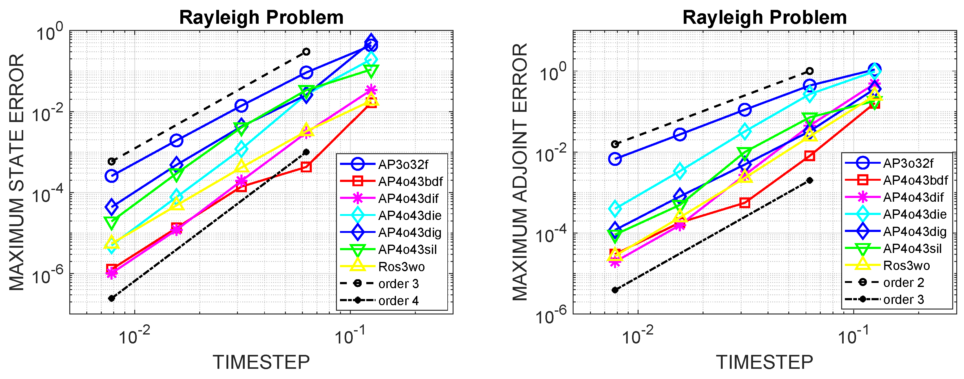
3.1. The Rayleigh Problem

The first problem is taken from [24] and describes the behaviour of a tunnel-diode oscillator. With the electric current $y_1\left(t\right)$ and the transformed voltage at the generator $u\left(t\right)$, the Rayleigh problem reads

$$\begin{array}{cc}\hfill \mathrm{M}\mathrm{i}\mathrm{n}\mathrm{i}\mathrm{m}\mathrm{i}\mathrm{z}\mathrm{e}{\int }_0^{2.5}\left(u{\left(t\right)}^2+y_1{\left(t\right)}^2\right)dt& \end{array}$$

(74)

$$\begin{array}{cc}\hfill \mathrm{s}\mathrm{u}\mathrm{b}\mathrm{j}\mathrm{e}\mathrm{c}\mathrm{t}\mathrm{t}\mathrm{o}{y}_1^{″}\left(t\right)-y_1^{\prime }\left(1.4-0.14y_1^{\prime }{\left(t\right)}^2\right)+y_1\left(t\right)=& 4u\left(t\right),t\in (0,2.5],\hfill \end{array}$$

(75)

$$\begin{array}{cc}\hfill y_1\left(0\right)=y_1^{\prime }\left(0\right)=& -5.\hfill \end{array}$$

(76)

Introducing $y_2\left(t\right)=y_1^{\prime }\left(t\right)$ and eliminating the control $u\left(t\right)$ yields the following nonlinear boundary value problem (see [5] for more details):

$$\begin{array}{cc}\hfill y_1^{\prime }\left(t\right)=& y_2\left(t\right),\hfill \end{array}$$

(77)

$$\begin{array}{cc}\hfill y_2^{\prime }\left(t\right)=& -y_1\left(t\right)+y_2\left(t\right)\left(1.4-0.14y_2{\left(t\right)}^2\right)-8p_2\left(t\right),\hfill \end{array}$$

(78)

$$\begin{array}{cc}\hfill & y_1\left(0\right)=-5,y_2\left(0\right)=-5,\hfill \end{array}$$

(79)

$$\begin{array}{cc}\hfill p_1^{\prime }\left(t\right)=& p_2\left(t\right)-2y_1\left(t\right),\hfill \end{array}$$

(80)

$$\begin{array}{cc}\hfill p_2^{\prime }\left(t\right)=& -p_1\left(t\right)-(1.4-0.42y_2{\left(t\right)}^2)p_2\left(t\right),\hfill \end{array}$$

(81)

$$\begin{array}{cc}\hfill & p_1\left(2.5\right)=0,p_2\left(2.5\right)=0.\hfill \end{array}$$

(82)

To study convergence orders of our new methods, we compute a reference solution at the discrete time points $t=t_n$ by applying the classical fourth-order RK4 with $N=1280$ steps. Numerical results for the maximum state and adjoint errors are presented in Figure 1 for $N+1=20,40,80,160,320$. AP3o32f and Ros3wo show their expected orders $(3,2)$ and $(3,3)$ for state and adjoint solutions, respectively. Order three for the adjoint solutions is achieved by all new four-stage Peer methods. The smaller error constants of AP4o43bdf, AP4o43dif and Ros3wo are clearly visible. The additional superconvergence order four for the state solutions shows up for AP4o43die and AP4o43sil and nearly for AP4o43dif and AP4o43dig. AP4o43bdf does not reach its full order four here, too.

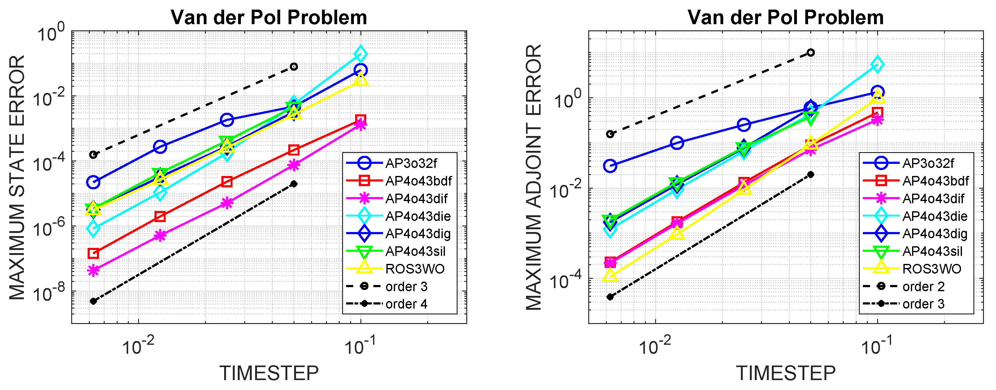
3.2. The van der Pol Oscillator

Our second problem is the following optimal control problem for the van der Pol oscillator:

$$\begin{array}{cc}\hfill \mathrm{M}\mathrm{i}\mathrm{n}\mathrm{i}\mathrm{m}\mathrm{i}\mathrm{z}\mathrm{e}{\int }_0^2\left(u{\left(t\right)}^2+y{\left(t\right)}^2+y^{\prime }{\left(t\right)}^2\right)dt& \end{array}$$

(83)

$$\begin{array}{cc}\hfill \mathrm{s}\mathrm{u}\mathrm{b}\mathrm{j}\mathrm{e}\mathrm{c}\mathrm{t}\mathrm{t}\mathrm{o}\epsilon y^{″}\left(t\right)-\left(1-y{\left(t\right)}^2\right)y^{\prime }\left(t\right)+y\left(t\right)=& u\left(t\right),t\in (0,2],\hfill \end{array}$$

(84)

$$\begin{array}{cc}\hfill y\left(0\right)=0,y^{\prime }\left(0\right)=& 2.\hfill \end{array}$$

(85)

Introducing Lienhardt’s coordinates $y_2\left(t\right)=y\left(t\right)$, $y_1\left(t\right)=\epsilon y^{\prime }\left(t\right)+y{\left(t\right)}^3/3-y\left(t\right)$, and eliminating the control $u\left(t\right)$, we finally get the following nonlinear boundary value problem in $[0,2]$ (see again [5] for more details):

$$\begin{array}{cc}\hfill y_1^{\prime }\left(t\right)=& -y_2\left(t\right)-\frac{p_1\left(t\right)}{2},\hfill \end{array}$$

(86)

$$\begin{array}{cc}\hfill y_2^{\prime }\left(t\right)=& \frac{1}{\epsilon }\left(y_1\left(t\right)+y_2\left(t\right)-\frac{y_2{\left(t\right)}^3}{3}\right),\hfill \end{array}$$

(87)

$$\begin{array}{cc}\hfill & y_1\left(0\right)=2\epsilon ,y_2\left(0\right)=0,\hfill \end{array}$$

(88)

$$\begin{array}{cc}\hfill p_1^{\prime }\left(t\right)=& -\frac{1}{\epsilon }{p}_2\left(t\right)-\frac{1}{{\epsilon }^2}\left(y_1\left(t\right)+y_2\left(t\right)-\frac{y_2{\left(t\right)}^3}{3}\right),\hfill \end{array}$$

(89)

$$\begin{array}{cc}\hfill p_2^{\prime }\left(t\right)=& p_1\left(t\right)-\frac{1}{\epsilon }\left(1-y_2{\left(t\right)}^2\right)p_2\left(t\right)\hfill \end{array}$$

(90)

$$\begin{array}{cc}\hfill & -\frac{2}{{\epsilon }^2}\left(y_1\left(t\right)+y_2\left(t\right)-\frac{y_2{\left(t\right)}^3}{3}\right)\left(1-y_2{\left(t\right)}^2\right)-2y_2\left(t\right),\hfill \end{array}$$

(91)

$$\begin{array}{cc}\hfill & p_1\left(2\right)=0,p_2\left(2\right)=0.\hfill \end{array}$$

(92)

The van der Pol equation with small positive values of $\epsilon$ gives rise to very steep profiles in $y\left(t\right)$, requiring variable step sizes for an efficient numerical approximation. Since the factor ${\epsilon }^{-2}$ appears in the adjoint equations, the boundary value problem is even harder to solve. In order to apply constant step sizes with $N+1=20,40,80,160,320$, we consider the mildly stiff case with $\epsilon =0.1$ for our convergence study.

Numerical results for the maximum state and adjoint errors are presented in Figure 2, where a reference solution is computed with AP4o43bdf for $N=1279$. Order three for the adjoint solutions is achieved by all new four-stage Peer methods and also by Ros3wo. The three-stage Peer method AP3o32f drops down to order $1.3$. For AP4o43dig and AP4o43sil applied with $N=19$, Matlab’s fsolve was not able to deliver a solution. The additional superconvergence order four for the state solutions is visible for AP4o43die and nearly for AP4o43dif which performs best and beats AP4o43bdf by a factor five. AP4o43bdf does not reach its full order four here. The methods AP4o43sil and AP4o43dig show order three only, whereas AP3o32f and Ros3wo reach their theoretical order three.

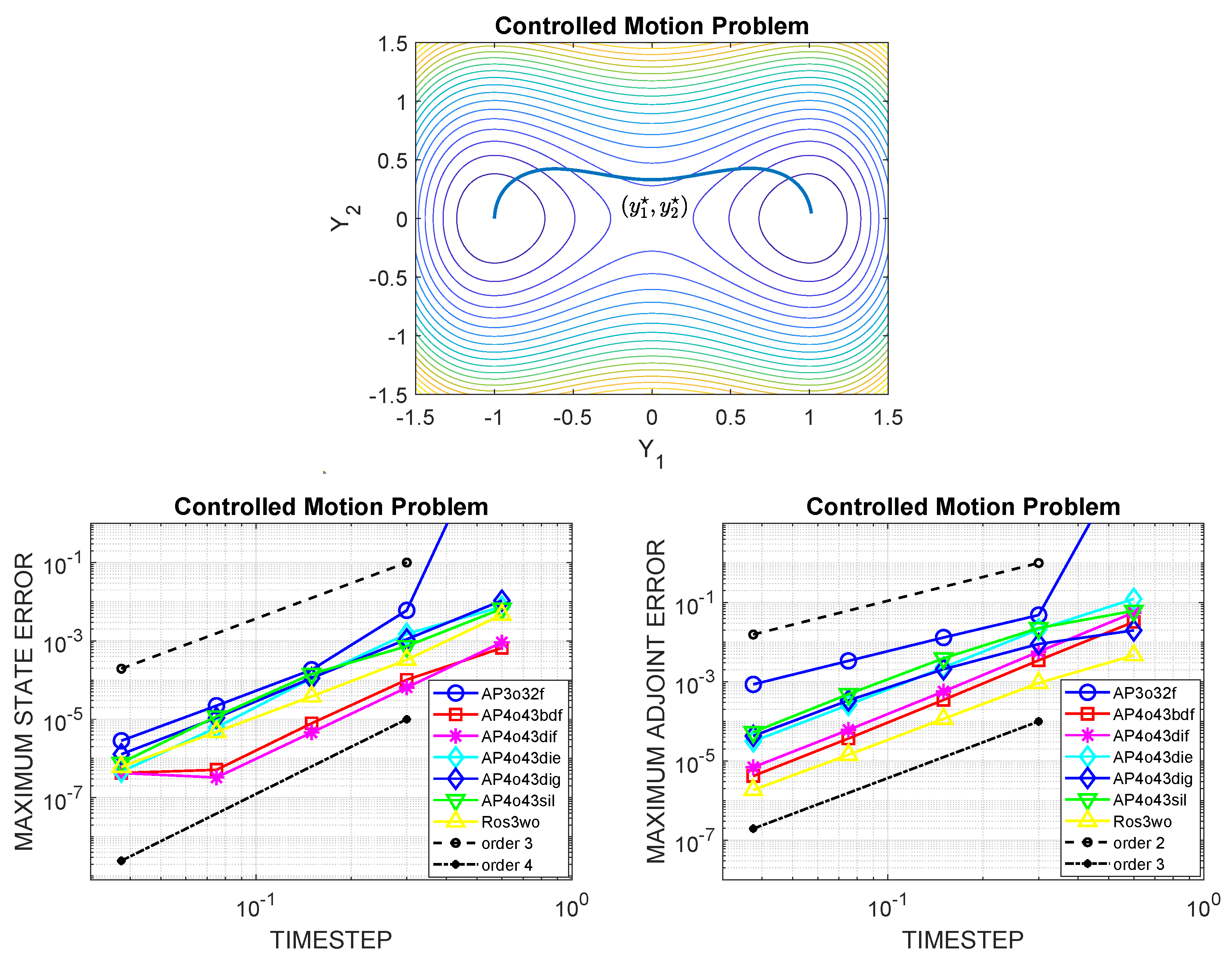
3.3. A Controlled Motion Problem

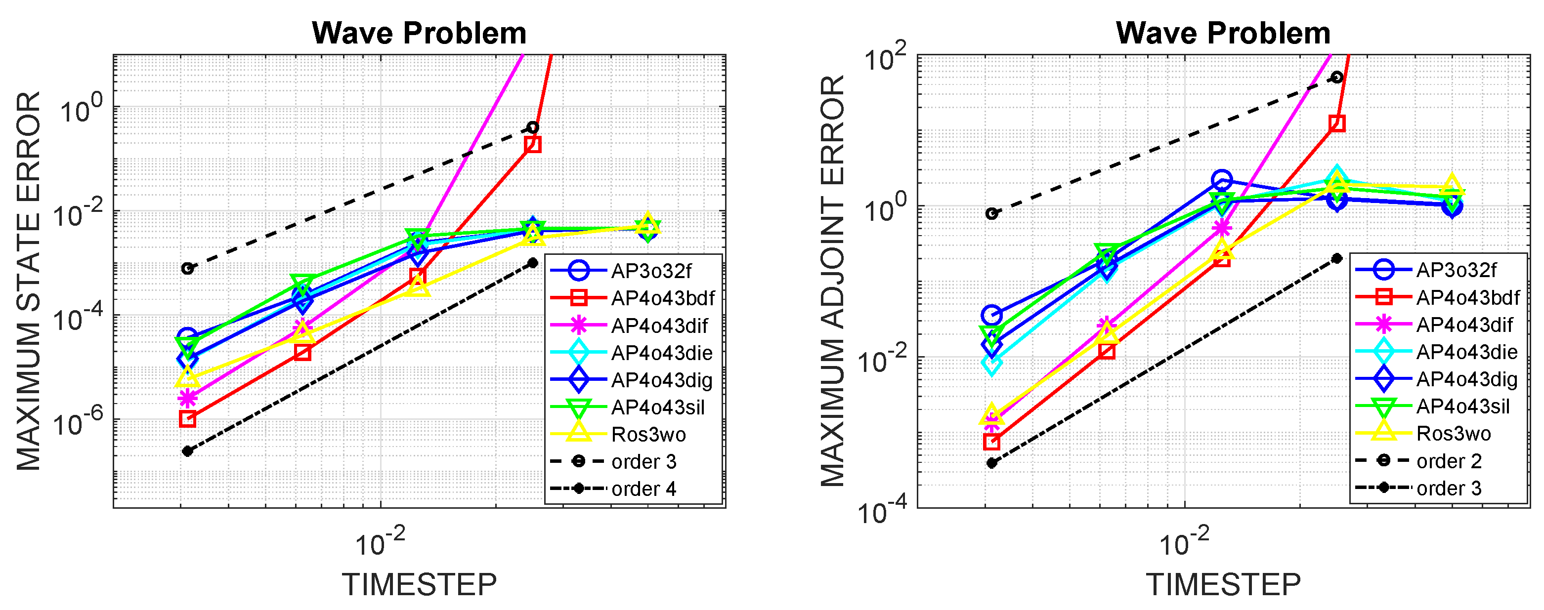
This problem was studied in [1]. The motion of a damped oscillator is controlled in a double-well potential, where the control $u\left(t\right)$ acts only on the velocity $y_2\left(t\right)$. The optimal control problem reads

$$\begin{array}{cc}\hfill \mathrm{M}\mathrm{i}\mathrm{n}\mathrm{i}\mathrm{m}\mathrm{i}\mathrm{z}\mathrm{e}\frac{\alpha }{2}{\parallel y\left(6\right)-y_f\parallel }^2+\frac{1}{2}{\int }_0^{6}u{\left(t\right)}^{2}dt& \end{array}$$

(93)

$$\begin{array}{cc}\hfill \mathrm{s}\mathrm{u}\mathrm{b}\mathrm{j}\mathrm{e}\mathrm{c}\mathrm{t}\mathrm{t}\mathrm{o}{y}_1^{\prime }\left(t\right)-y_2\left(t\right)=& 0,\hfill \end{array}$$

(94)

$$\begin{array}{cc}\hfill y_2^{\prime }\left(t\right)-y_1\left(t\right)+y_1{\left(t\right)}^3+\nu y_2\left(t\right)=& u\left(t\right),t\in (0,6],\hfill \end{array}$$

(95)

$$\begin{array}{cc}\hfill y_1\left(0\right)=-1,y_2\left(0\right)=& 0,\hfill \end{array}$$

(96)

where $\nu >0$ is the damping parameter and $y_f$ the target final position. As in [1], we set $\nu =1$, $y_f={(1,0)}^{\mathsf{T}}$, and $\alpha =10$.

Eliminating the scalar control $u\left(t\right)$ yields the following nonlinear boundary value problem:

$$\begin{array}{cc}\hfill y_1^{\prime }\left(t\right)=& y_2\left(t\right),\hfill \end{array}$$

(97)

$$\begin{array}{cc}\hfill y_2^{\prime }\left(t\right)=& y_1\left(t\right)-y_1{\left(t\right)}^3-\nu y_2\left(t\right)-p_2\left(t\right),\hfill \end{array}$$

(98)

$$\begin{array}{cc}\hfill & y_1\left(0\right)=-1,y_2\left(0\right)=0,\hfill \end{array}$$

(99)

$$\begin{array}{cc}\hfill p_1^{\prime }\left(t\right)=& (3y_1{\left(t\right)}^2-1)p_2\left(t\right),\hfill \end{array}$$

(100)

$$\begin{array}{cc}\hfill p_2^{\prime }\left(t\right)=& -p_1\left(t\right)+\nu p_2\left(t\right),\hfill \end{array}$$

(101)

$$\begin{array}{cc}\hfill & p_1\left(6\right)=\alpha (y_1\left(6\right)-1),p_2\left(6\right)=\alpha y_2\left(6\right).\hfill \end{array}$$

(102)

The optimal control $u^{☆}=-p_2^{☆}$ must accelerate the motion of the particle to follow an optimal path $(y_1^{☆},y_2^{☆})$ through the total energy field $E=\frac{1}{2}{y}_2^2+\frac{1}{4}{y}_1^4-\frac{1}{2}{y}_1^2$, shown in Figure 3 on the top, in order to reach the final target $y_f$ behind the saddle point. The cost obtained from a reference solution with $N=1279$ is $C\left(y\right(6\left)\right)=0.77674$, which is in good agreement with the lower order approximation in [1]. Numerical results for the maximum state and adjoint errors are presented in Figure 3 for $N+1=10,20,40,80,160$. Worthy of mentioning is the repeated excellent performance of AP4o43bdf and AP4o43dif, but also the convincing results achieved by the third-order method Ros3wo. All theoretical orders are well observable, except for AP4o43dig, which tends to order three for the state solutions. A closer inspection reveals that this is caused by the second state $y_2$, while the first one asymptotically converges with fourth order. However, the three methods AP4o43die, AP4o43dig, and AP4o43sil perform quite similar. Observe that AP3o32f has convergence problems for $N=9$.

The stagnation of the state errors for the finest step sizes is due to the limited accuracy of Matlab’s fsolve—a fact which was already reported in [17].

3.4. A Wave Problem

The fourth problem is taken from [25] and demonstrates the practical importance of A-stability. We consider the optimal control problem

$$\begin{array}{cc}\hfill \mathrm{M}\mathrm{i}\mathrm{n}\mathrm{i}\mathrm{m}\mathrm{i}\mathrm{z}\mathrm{e}{y}_1\left(1\right)+\frac{1}{2}{\int }_0^{1}u{\left(t\right)}^{2}dt& \end{array}$$

(103)

$$\begin{array}{cc}\hfill \mathrm{s}\mathrm{u}\mathrm{b}\mathrm{j}\mathrm{e}\mathrm{c}\mathrm{t}\mathrm{t}\mathrm{o}{y}_1^{″}\left(t\right)+{\left(2\pi \kappa \right)}^2{y}_1\left(t\right)=& u\left(t\right),t\in (0,1],\hfill \end{array}$$

(104)

$$\begin{array}{cc}\hfill y_1\left(0\right)=y_1^{\prime }\left(0\right)=& 0,\hfill \end{array}$$

(105)

where $\kappa =16$ is used. Introducing $y_2\left(t\right)=y_1^{\prime }\left(t\right)$ and eliminating the control $u\left(t\right)$ yields the following linear boundary value problem:

$$\begin{array}{cc}\hfill y_1^{\prime }\left(t\right)=& y_2\left(t\right),\hfill \end{array}$$

(106)

$$\begin{array}{cc}\hfill y_2^{\prime }\left(t\right)=& -{\left(2\pi \kappa \right)}^2{y}_1\left(t\right)-p_2\left(t\right),\hfill \end{array}$$

(107)

$$\begin{array}{cc}\hfill & y_1\left(0\right)=0,y_2\left(0\right)=0,\hfill \end{array}$$

(108)

$$\begin{array}{cc}\hfill p_1^{\prime }\left(t\right)=& {\left(2\pi \kappa \right)}^2{p}_2\left(t\right),\hfill \end{array}$$

(109)

$$\begin{array}{cc}\hfill p_2^{\prime }\left(t\right)=& -p_1\left(t\right),\hfill \end{array}$$

(110)

$$\begin{array}{cc}\hfill & p_1\left(1\right)=1,p_2\left(1\right)=0.\hfill \end{array}$$

(111)

The exact solutions are given by

$$\begin{array}{cc}\hfill y_1^{*}\left(t\right)=& \frac{1}{2{\left(2\pi \kappa \right)}^3}sin\left(2\pi \kappa t\right)-\frac{t}{2{\left(2\pi \kappa \right)}^2}cos\left(2\pi \kappa t\right),\hfill \end{array}$$

(112)

$$\begin{array}{cc}\hfill y_2^{*}\left(t\right)=& \frac{t}{2\left(2\pi \kappa \right)}sin\left(2\pi \kappa t\right),\hfill \end{array}$$

(113)

$$\begin{array}{cc}\hfill p_1^{*}\left(t\right)=& cos\left(2\pi \kappa t\right),p_2^{*}\left(t\right)=\frac{1}{2\pi \kappa }sin\left(2\pi \kappa t\right),\hfill \end{array}$$

(114)

and the optimal control is $u^{*}\left(t\right)=-p_2^{*}\left(t\right)$. The key observation here is that the eigenvalues of the Jacobian of the right-hand side in (106)–(111) are ${\lambda }_{1/2}=2\pi \kappa i$ and ${\lambda }_{3/4}=-2\pi \kappa i$, which requests appropriate step sizes for only the $A(\alpha$)-stable methods AP4o43bdf and AP4o34dif due to their stability restrictions along the imaginary axis. Indeed, a closer inspection of the stability region of the (multistep) BDF4 method near the origin reveals that $|\lambda h_{bdf4}|\le 0.3$ is a minimum requirement to achieve acceptable approximations for problems with imaginary eigenvalues and moderate time horizon. For the four-stage AP4o43bdf with step size $h=4h_{bdf4}$, this yields $\left|\lambda h\right|\le 1.2$ and hence $h\le 1/\left(32\pi \right)\approx 0.02$ for the wave problem considered. A similar argument applies to AP4o34dif, too. Numerical results for the maximum state and adjoint errors are plotted in Figure 4 for $N+1=20,40,80,160,320$. They clearly show that both methods deliver first feasible results for $h=1/80$ and below only, but then again outperform the other Peer methods. Once again, Ros3wo performs remarkably well. The orders of convergence for the adjoint solutions are one better than the theoretical values, possibly due to the overall linear structure of the boundary value problem.

4. Discussion

We have extended our three-stage adjoint Peer two-step methods constructed in [13] to four stages to not only improve the convergence order of the methods but also their stability. Combining superconvergence of a standard Peer method with a careful design of starting and end Peer methods with appropriately enhanced structure, discrete adjoint A-stable Peer methods of order (4,3) could be found. Still, new requirements had to be dealt with for the higher order pair (4,3). The property of A-stability comes with larger error constants and a few other minor structural disadvantages. As long as A-stability is not an issue to solve the boundary value problem arising from eliminating the control from the system of KKT conditions, a Peer variant AP4o43bdf of the $A\left({73.35}^{\circ }\right)$-stable BDF4 and the $A\left({84}^{\circ }\right)$-stable AP4o43dif are the most attractive methods, which perform equally well depending on the problem type. The A-stable methods AP4o43dig and AP4o43die with diagonally implicit standard Peer methods are very good alternatives if eigenvalues close or on the imaginary axis are existent. We have also constructed the A-stable method AP4o43sil with a singly-diagonal main part as an additional option if large linear systems can be still solved by a direct solver and hence the property of requesting one LU-decomposition only is highly valuable. In future work, we plan to train our novel methods in a projected gradient approach to also tackle large-scale PDE constrained optimal control problems with semi-discretizations in space. In these applications, Peer triplets may have to satisfy even more severe requirements.

References

1. Liu, X.; Frank, J. Symplectic Runge-Kutta discretization of a regularized forward-backward sweep iteration for optimal control problems. J. Comput. Appl. Math. 2021, 383, 113133. [Google Scholar] [CrossRef]
2. Sanz-Serna, J. Symplectic Runge–Kutta schemes for adjoint equations, automatic differentiation, optimal control, and more. SIAM Rev. 2016, 58, 3–33. [Google Scholar] [CrossRef]
3. Hairer, E.; Wanner, G.; Lubich, C. Geometric Numerical Integration, Structure-Preserving Algorithms for Ordinary Differential Equations; Springer Series in Computational Mathematic; Springer: Berlin/Heidelberg, Germany, 1970; Volume 31. [Google Scholar]
4. Matsuda, T.; Miyatake, Y. Generalization of partitioned Runge–Kutta methods for adjoint systems. J. Comput. Appl. Math. 2021, 388, 113308. [Google Scholar] [CrossRef]
5. Lang, J.; Verwer, J. W-Methods in Optimal Control. Numer. Math. 2013, 124, 337–360. [Google Scholar] [CrossRef]
6. Almuslimani, I.; Vilmart, G. Explicit stabilized integrators for stiff optimal control problems. SIAM J. Sci. Comput. 2021, 43, A721–A743. [Google Scholar] [CrossRef]
7. Lubich, C.; Ostermann, A. Runge-Kutta approximation of quasi-linear parabolic equations. Math. Comp. 1995, 64, 601–627. [Google Scholar] [CrossRef]
8. Ostermann, A.; Roche, M. Runge-Kutta methods for partial differential equations and fractional orders of convergence. Math. Comp. 1992, 59, 403–420. [Google Scholar] [CrossRef]
9. Gerisch, A.; Lang, J.; Podhaisky, H.; Weiner, R. High-order linearly implicit two-step peer—Finite element methods for time-dependent PDEs. Appl. Numer. Math. 2009, 59, 624–638. [Google Scholar] [CrossRef]
10. Gottermeier, B.; Lang, J. Adaptive Two-Step Peer Methods for Incompressible Navier-Stokes Equations. In Proceedings of the ENUMATH 2009, the 8th European Conference on Numerical Mathematics and Advanced Applications, Uppsala, Sweden, 29 June–3 July 2009; Kreiss, G., Lötstedt, P., Malqvist, A., Neytcheva, M., Eds.; Springer: Berlin/Heidelberg, Germany, 2009; pp. 387–395. [Google Scholar]
11. Albi, G.; Herty, M.; Pareschi, L. Linear multistep methods for optimal control problems and applications to hyperbolic relaxation systems. Appl. Math. Comput. 2019, 354, 460–477. [Google Scholar] [CrossRef]
12. Sandu, A. Reverse automatic differentiation of linear multistep methods. In Advances in Automatic Differentiation; Lecture Notes in Computational Science and Engineering; Bischof, C., Bücker, H., Hovland, P., Naumann, U., Utke, J., Eds.; Springer: Berlin/Heidelberg, Germany, 2008; Volume 64, pp. 1–12. [Google Scholar]
13. Lang, J.; Schmitt, B. Discrete adjoint implicit peer methods in optimal control. J. Comput. Appl. Math. 2022, 416, 114596. [Google Scholar] [CrossRef]
14. Hager, W. Runge-Kutta methods in optimal control and the transformed adjoint system. Numer. Math. 2000, 87, 247–282. [Google Scholar] [CrossRef]
15. Troutman, J. Variational Calculus and Optimal Control; Springer: New York, NY, USA, 1996. [Google Scholar]
16. Bonnans, F.; Laurent-Varin, J. Computation of order conditions for symplectic partitioned Runge-Kutta schemes with application to optimal control. Numer. Math. 2006, 103, 1–10. [Google Scholar] [CrossRef]
17. Herty, M.; Pareschi, L.; Steffensen, S. Implicit-Explicit Runge-Kutta schemes for numerical discretization of optimal control problems. SIAM J. Numer. Anal. 2013, 51, 1875–1899. [Google Scholar] [CrossRef]
18. Sandu, A. On the properties of Runge-Kutta discrete adjoints. Lect. Notes Comput. Sci. 2006, 3394, 550–557. [Google Scholar]
19. Schröder, D.; Lang, J.; Weiner, R. Stability and consistency of discrete adjoint implicit peer methods. J. Comput. Appl. Math. 2014, 262, 73–86. [Google Scholar] [CrossRef]
20. Montijano, J.; Podhaisky, H.; Randez, L.; Calvo, M. A family of L-stable singly implicit Peer methods for solving stiff IVPs. BIT 2019, 59, 483–502. [Google Scholar] [CrossRef]
21. Schmitt, B.; Weiner, R. Efficient A-stable peer two-step methods. J. Comput. Appl. Math. 2017, 316, 319–329. [Google Scholar] [CrossRef]
22. Schmitt, B. Algebraic criteria for A-stability of peer two-step methods. Technical Report. arXiv 2015, arXiv:1506.05738. [Google Scholar]
23. Jackiewicz, Z. General Linear Methods for Ordinary Differential Equations; John Wiley&Sons: Hoboken, NJ, USA, 2009. [Google Scholar]
24. Jacobson, D.; Mayne, D. Differential Dynamic Programming; American Elsevier Publishing: New York, NY, USA, 1970. [Google Scholar]
25. Dontchev, A.; Hager, W.; Veliov, V. Second-order Runge-Kutta approximations in control constrained optimal control. SIAM J. Numer. Anal. 2000, 38, 202–226. [Google Scholar] [CrossRef]
Figure 1. Rayleigh Problem: Convergence of the maximal state errors ( w T I ) Y n y ( t n + 1 ) (left) and adjoint errors ( v T I ) P n p ( t n ) (right), n = 0 , , N .
Algorithms 15 00310 g001
Figure 2. Van der Pol Problem: Convergence of the maximal state errors ( w T I ) Y n y ( t n + 1 ) (left) and adjoint errors ( v T I ) P n p ( t n ) (right), n = 0 , , N .
Algorithms 15 00310 g002
Figure 3. Controlled Motion Problem: optimal path ( y 1 , y 2 ) through the total energy field E = 1 2 y 2 2 + 1 4 y 1 4 1 2 y 1 2 visualized by isolines and exhibiting a saddle point structure (top). Convergence of the maximal state errors ( w T I ) Y n y ( t n + 1 ) (bottom left) and adjoint errors ( v T I ) P n p ( t n ) (bottom right), n = 0 , , N .
Algorithms 15 00310 g003
Figure 4. Wave Problem: Convergence of the maximal state errors ( w T I ) Y n y ( t n + 1 ) (left) and adjoint errors ( v T I ) P n p ( t n ) (right), n = 0 , , N .
Algorithms 15 00310 g004