Optimal Algorithms for Sorting Permutations with Brooms

Abstract

Sorting permutations with various operations has applications in genetics and computer interconnection networks where an operation is specified by its generator set. A transposition tree $T=(V,E)$ is a spanning tree over n vertices $v_1,v_2,\dots v_n$. T denotes an operation in which each edge is a generator. A value assigned to a vertex is called a token or a marker. The markers on vertices u and v can be swapped only if the pair $(u,v)\in E$. The initial configuration consists of a bijection from the set of vertices $v_1,v_2,\dots ,v_n$ to the set of markers $(1,2,\cdots ,n-1,n)$. The goal is to sort the initial configuration of T, i.e., an input permutation, by applying the minimum number of swaps or moves in T. Computationally tractable optimal algorithms to sort permutations are known only for a few classes of transposition trees. We study a class of transposition trees called a broom and its variation a double broom. A single broom is a tree obtained by joining the centre vertex of a star with one of the two leaf vertices of a path graph. A double broom is an extension of a single broom where the centre vertex of a second star is connected to the terminal vertex of the path in a single broom. We propose a simple and efficient algorithm to obtain an optimal swap sequence to sort permutations with the transposition tree broom and a novel optimal algorithm to sort permutations with a double broom. We also introduce a new class of trees named millipede tree and prove that $D^{*}$ yields a tighter upper bound for sorting permutations with a balanced millipede tree compared to $D^{\prime }$. Algorithms $D^{*}$ and $D^{\prime }$ are designed previously.

1. Introduction

Sorting permutations with various operations has applications in genetics and computer interconnection networks [1,2,3,4] and is an active field of research.Reversals, transpositions, prefix reversals, prefix transpositions have been extensively studied with respect to upper bounds, lower bounds, exact distances for all permutations in $S_n$ etc. Transposition tree is one such operation which has applications in solving puzzles and robot motion planning [5,6].

Hypercube architecture was a golden standard in 1980s for computer interconnection networks. Later, Akers and Krishnamurthy [1] proposed a transposition tree called star, and showed that the Cayley graph corresponding to star, called star graph can accommodate $n!$ nodes and has diameter sub-logarithmic in number of vertices. Star graphs surpass the then topology Hypercube, both in scalability and diameter because the later can accommodate only $2^n$ vertices and has diameter logarithmic in number of vertices. Diameter is an important quality of service parameter deciding the latency of interconnection networks [7,8]. There is a natural trade-off between diameter and the cardinality of the generator set. That is, a larger generator set decreases the diameter and vice-versa. The diameter of a Cayley graph $\mathsf{\Gamma }$, can be trivially reduced to 1 if the degree of each node in $\mathsf{\Gamma }$ is one less than the total number of nodes. However, if the number of symbols, i.e., the label length of a vertex is n, then this would require the degree to be $n!-1$ and this is infeasible. Thus, a good balance is sought. In this regard, the degree of $\mathsf{\Gamma }$ generated using any transposition tree is a relatively small value of $n-1$ and for some trees the diameter can be small as well. For example, for a star graph the diameter is $3/2n+O\left(1\right)$ [1]. Thus, Cayley networks were established as a better topology than hypercubes for interconnection networks. Cayley networks also possess other desirable features such as vertex symmetry and small diameter [1]. These are detailed in Heydemann [3], Lakshmivarahan et al. [4], and Xu [8].

In this article we study the problem of sorting permutations under the operation specified by specific transposition trees—single broom, double broom and millipede tree. A transposition tree $T=(V,E)$ is a spanning tree over n vertices $v_1,v_2,\dots ,v_n$. T denotes an operation in which each edge is a generator [1]. A value assigned to a vertex is called token or marker. The markers on vertices u and v can be swapped only if the pair $(u,v)\in E$. This is equivalent to applying the corresponding generator and is referred to as making a move. Since swap is symmetric, the edge $(u,v)$ is undirected. The initial configuration consists of a bijection from $v_1,v_2,\dots v_n$ to $(1,2,\cdots ,n-1,n)$; i.e., from the set of vertices to the set of markers over the alphabet $\{1,2,\cdots ,n-1,n\}$. That is, one can view each vertex $v_i$ as an index i in an array where some marker j resides. Thus, input consists of a permutation. The vertex $v_i$ is the home for the corresponding marker i and we seek to home all markers with minimum number of moves. Note that if for all i, $v_i=i$ then the permutation is sorted. Thus, the goal is to sort the initial configuration, i.e., an input permutation, by applying the minimum number of generators (or swaps or moves) of T. In the remainder of the article, ‘sorting’ refers to transforming a given permutation into the identity permutation with a minimum number of moves of T.

Example 1. 

LetTbe a transposition tree with$V=\{1,2,3,4,5\}$and$E=\left\{\right(1,2\left)\right(2,3\left)\right(3,4)$$(4,5)\}$. The generators are the permutations$\left\{\right(21345),(13245),(12435),(12354\left)\right\}$.

The computational complexity of sorting permutations with transposition trees is unknown in general. However, computationally tractable optimal algorithms to sort permutations are known for a few classes of transposition trees such as star [1], path [9], broom [5,6,10], etc.

We study the problem of sorting permutations with a single broom and a double broom transposition trees. A broom, also referred to as a single broom, is a transposition tree obtained by joining the center vertex of a star with one of the leaf vertices of a path. Several efficient optimal algorithms are known to sort permutations using a broom [5,10,11]. In Section 3 we design a new efficient optimal algorithm for sorting permutations using single broom. In Section 4 we design a novel efficient optimal algorithm for sorting permutations using double brooms. This algorithm is designed by extending the algorithm for single broom. The problem of sorting permutations using a new class of trees called millipede tree, is studied in Section 5. Section 6 demonstrates the limitation of the proposed algorithms when performed on an n-Broom providing a new direction for future research in the field of sorting permutations using transposition trees.

2. Preliminaries and Background

In this article, we employ the alphabet $\{1,2,\cdots ,n-1,n\}$ to generate the symmetric group $S_n$. The permutation $I=(1,2,3,4,\cdots ,n-1,n)$ is the identity permutation in $S_n$. An operation $\mathcal{G}$ is specified by a generator set that is a subset of $S_n$; $\mathcal{G}\subset S_n$. Each permutation in the generator set is a generator. Let $\pi$ be a permutation in $S_n$, and $\sigma$ be a generator. Applying $\sigma$ on $\pi$ yields another permutation, say $\gamma \in S_n$. We say that $\sigma$ transforms $\pi$ into $\gamma$. Given two permutations $\alpha ,\beta \in S_n$, and an operation $\mathcal{G}$, the minimum number of generators of $\mathcal{G}$ required to transform $\alpha$ into $\beta$ is called the distance from $\alpha$ to $\beta$ under $\mathcal{G}$, denoted by $d_{\mathcal{G}}(\alpha ,\beta )$ and in general, it is hard to compute the same if the number of generators is two or more [12]. When $\mathcal{G}$ is symmetric, then $d_{\mathcal{G}}(\alpha ,\beta )=d_{\mathcal{G}}(\beta ,\alpha )$. If the target permutation is I, then $d_{\mathcal{G}}(\alpha ,I)$ is succinctly denoted as $d_{\mathcal{G}}\left(\alpha \right)$, which is called the distance of $\alpha$. Transforming $\alpha$ into I is called as sorting $\alpha$, and thus $d_{\mathcal{G}}\left(\alpha \right)$ is the number of generators required to sort $\alpha$ parsimoniously. Let $g_1,g_2,\dots g_t$ be a shortest sequence of generators such that $\alpha \circ g_1\circ g_2\dots g_t=\beta$. Then ${\beta }^{-1}\circ \alpha \circ g_1\circ g_2\dots g_t={\beta }^{-1}\circ \beta =I$. That is, the number of moves required to transform $\alpha$ into $\beta$ is same as that of transforming ${\beta }^{-1}\circ \alpha$ into the identity permutation I. Thus, the problem of finding minimum distance between two given permutations reduces to the problem of sorting a related permutation. If the target permutation is I, then $d_{\mathcal{G}}({\beta }^{-1}\circ \alpha ,I)$ is denoted as $d_{\mathcal{G}}({\beta }^{-1}\circ \alpha )$, which is called the distance of a single permutation ${\beta }^{-1}\circ \alpha$.

Various operations have been studied in the past. Some of them are reversal, transposition, block interchange, etc. A block move operation moves a block; e.g., block transposition, suffix block transposition etc. A small sample of the research in this broad area follows. Christie studied sorting permutations by transpositions and proved a tighter lower bound based on the hurdles of the underlying cycle graph and designed a simpler 3/2-approximation algorithm [13]. The first non-trivial lower and upper bounds for prefix transposition distance over permutations were given in [2]. Chitturi et al. [14] shows how to compute the transposition distances of all permutations in $S_n$ in an amortized time of $O\left(n^3\right)$. Recently, subsets of permutations related to a certain type of block move operation have been counted [15]. These results are varied in type that employ distinct techniques such as dynamic programming and applications of graph properties, and constructs such as cycle graphs and adjacencies in permutations.

A Cayley graph ${\mathsf{\Gamma }}_T$ under the operation T over $S_n$ is defined as follows. The vertex set V of ${\mathsf{\Gamma }}_T$ consists of all permutations in $S_n$. There is an edge from vertex u to vertex v if there is a generator $g\in T$ such that $ug=v$. The distance between two permutations $\alpha$, and $\beta$ under the operation T, $d_T(\alpha ,\beta )$ is equal to the number of edges in the shortest path between the corresponding vertices in ${\mathsf{\Gamma }}_T$. The diameter of ${\mathsf{\Gamma }}_T$, $D_T\left(n\right)=ma{x}_{u,v\in S_n}{d}_T(u,v)$. A transposition tree in turn gives rise to a Cayley graph (refer Figure 1).

The problem of sorting permutations using transposition trees is also known as token swapping on trees [5,6,11,16,17,18,19]. Given a tree T consisting of n vertices $\{v_1,v_2,\dots v_n\}$ and edge set E, a configuration of T is an assignment of n distinct markers or tokens $\{1,2\dots n\}$ to the vertices of T. Tokens can be moved along the tree edges only. Given an initial configuration $f_i$ and a target configuration $f_t$ of a tree T, token swapping problem is to transform T from $f_i$ to $f_t$ with minimum number of moves.

A transposition tree with vertex set $\{v_1,v_2\dots v_n\}$ and edge set $\{(v_1,v_2),(v_2,v_3)\dots (v_{n-1},$$v_n\left)\right\}$ is called a path of length n. An optimal algorithm for sorting permutations using path requires k moves where k is the number of inversions in the given permutation [20]. The reverse permutation $(n,n-1,n-2\dots 1)$ is the diametral permutation of $S_n$ that requires $n(n-1)/2$ moves to sort. Another transposition tree studied in the past is star. A star (with center, say $v_1$) is a transposition tree with vertex set $\{v_1,v_2\dots v_n\}$ and edge set $\{(v_1,v_2),(v_1,v_3)\dots (v_1,v_n)\}$. Efficient optimal algorithms for sorting permutations using a star are known [1,21,22]. The optimum number of moves required to sort permutations using star is $m+c$, where m is the number of un-homed leaf markers, and c is the number of permutation cycles of length $\ge 2$, in the given permutation, consisting of un-homed leaf markers only [5]. When all cycles in a given permutation are of length 2, it takes the maximum number of moves to sort that permutation. Thus, the diameter of star graph is $\lfloor 3/2(n-1)\rfloor$ [1].

Generic algorithms to compute upper bounds (not necessarily tight) for sorting permutations with any given transposition tree have been studied. Akers and Krishnamurthy [1] propose the first known such algorithm that require exponential running time. Ganesan [23] proposed a method to compute an upper bound ${\beta }_{max}$ in exponential time which is an estimate of the upper bound by analyzing the structure of the transposition tree. Chitturi [24] designed two polynomial (O$\left(n^2\right)$) time algorithms, $\gamma$ and ${\delta }^{\prime }$ for computing upper bounds. The cumulative sum of upper bound values of $\gamma$ and ${\delta }^{\prime }$ for all trees of a particular size were found to be tighter than the values provided by earlier methods. Furthermore, these algorithms solely analyzed the structure of the tree and were computationally efficient. Kraft [25] proposed randomized algorithms with polynomial running time which were looser than the other upper bounds. Uthan and Chitturi define a class of trees called $S_{m,k}$ [26] and prove an exact upper bound for the same.

3. Sorting Permutations with a Single Broom

In this section, we design a polynomial time optimal algorithm for sorting permutations using a single broom. A single broom is a tree obtained by joining the center vertex of a star with one of the two leaf vertices of a path graph, using a new edge. A single broom has n vertices, partitioned into two sets called star vertices $v_1,v_2,\dots ,v_k$, and path vertices $v_{k+1},\dots ,v_n$, where $2\le k\le (n-3)$. Note that the center of the star, i.e., $v_{k+1}$ is also a path node. Similarly, markers are partitioned into two sets called star markers and path markers. A star marker is a marker whose home is a star node, and a path marker is a marker whose home is a path node. A new efficient optimal algorithm called $A_b$, for sorting permutations using single broom is given in Section 3.1.

3.1. Algorithm $A_b$

Let $S_{min}$ be the star marker that is closest to its home residing on the path and $P_{max}$ be the largest path marker that is not homed. Our algorithm $A_b$ for single broom that transforms a given input configuration to a sorted configuration, consists of the following 3 steps in the given order.

• While (∃ a $S_{min}$), efficiently home $S_{min}$;
• While (∃ a $P_{max}$), efficiently home $P_{max}$;
• Efficiently home the markers in the star that need to be homed.

An illustration of algorithm $A_b$ for a single broom is given in Figure 2. In the initial setup, we have two unhomed star markers on path, i.e., 3 on $v_7$ and 2 on $v_8$. $S_{min}$ is 3 in the first iteration and in the next it will be 2. Homing markers 3 and 2 take 5 swaps in total. Then, there will be no star markers residing on the path. Thus, we can start with Step 2 of our algorithm. $P_{max}$ is 8 and a swap with 7 homes both the markers. Only the star markers 5 and 4 at $v_4$ and $v_5$ respectively need to be homed. Our algorithm homes all markers in total of 9 swaps, exactly the same number of swaps that are taken by the algorithms of Biniaz et al. [5], Yamanaka et al. [6] and Vaughan [10].

Step 1 and Step 2 of $A_b$ have the following properties:

• Star markers residing on the path always move to the left in the increasing order of their distances from their respective homes;
• A path marker moves right to its home; thereby moving the smaller path markers towards the center;
• Swap involving two star markers will not take place on a path edge.

The next section covers the analysis and correctness proof of the algorithm $A_b$.

3.2. Analysis of $A_b$

We begin our analysis for the number of swaps with Step 1. Let $D\left(S_p\right)$ be the distance from $S_p$ to its home, where $S_p$ are the star markers residing on the path of the broom. $S_p$, can reside either on the central node or on the rest of the nodes in the path. Note that homing a marker from central node to a star leaf takes exactly a single swap. $W_s$ is the total number of swaps executed in Step 1. Since, we home the nearest markers first, the distances of the markers that are homed subsequently do not increase. Thus, we have the following expression.

$$W_s=\sum _{S_p}D\left(S_p\right).$$

Observe that for Step 2, we are now left only with the path containing path markers. The total moves required on the path to place the markers at their desirable vertices is same as the number of inversions [9,27,28]. Let $D\left(P_p\right)$ be the distance from the path marker $P_p$ to its home, where $P_p$ is the path marker residing on the path of the broom. $W_p$ is the total number of swaps executed in Step 2. Then, for the reason stated for $W{}_s$ in Step 1,

$$W{}_p=\sum _{P{}_p}D\left(P{}_p\right).$$

For the final step in $A_b$, let $L_S$ be the number of permutation cycles not containing the center vertex that have a length ≥ 2 and $N_S$ be the number of markers in these cycles. These markers are not swapped in Step 1 or Step 2. So, as discussed before in Section 2, the number of swaps to home the star markers is $L_S+N_S$.

$W_b$, the total number of swaps performed in $A_b$ is:

$$W{}_b=\sum _{P{}_p}D\left(P{}_p\right)+\sum _{S{}_p}D\left(S{}_p\right)+L{}_S+N{}_S.$$

Step 1 of $A_b$ takes a distance-based approach in which $S_{min}$ is selected on the basis of its distance from the leaf nodes in the star. Step 2 obeys a value-based approach in which a maximum valued path marker is homed first. Biniaz’s, Kawahara’s and Vaughan’s algorithms are strictly based on a value-based approach and work in $O\left(n^2\right)$ time. Figure 3 compares the traversal of markers in $A_b$ with the algorithms proposed by Biniaz and Kawahara.

Time complexity of $A_b$ can be expressed in terms of number of moves. The total number of $S_{min}$ markers possible in Step 1 is $min(S,P)$ where S is the number of star vertices and P is the number of path vertices. The worst case of this step occurs when all the path nodes are occupied by star markers and the homes of these star markers are occupied by other star markers. The total number of moves required in Step 1 is $\left(P\right(P+1)/2)+(S-P)$. The worst case of Step 2 occurs when all P path markers need to be homed with a total swap count of $P(P-1)/2$. Solving the star in step 3 requires a maximum of $\lfloor 3S/2\rfloor$ moves. Since $P,S\in O\left(n\right)$, Algorithm $A_b$ runs in $O\left(n^2\right)$ time.

As the number of edges in a single broom is $n-1$, the tree requires $O\left(n\right)$ space, and the algorithm does not require any additional space.

3.3. Correctness of $A_b$

In this section, we prove that $A_b$ finds an optimal swap sequence, $S_{opt}$, which always follows some interesting properties. To show that, $S_{opt}$ is optimal, we first prove that these properties hold for a given marker on a broom and then apply induction on n.

Lemma 1.

An optimal path sequence $S_{opt}$ will obey following properties:

• A pair of markers swap at most once.
  Proof. 

  We prove it using contradiction. Suppose the swap sequence $S=S_1,S_2,S_3\dots S_s$, contains the swap of $(x,y)$ twice at $S_i$ and $S_j$. Modify S by deleting $S_i$ and $S_j$. Then, for each swap $S_k$ where $i<k<j$, replace x with y and vice-versa. Resulting swap sequence is shorter and achieves the same results.    □
• Star markers that enter the star from path do so in the increasing order of their distance from center.
  Proof. 

  Consider two star markers x and y residing on the path. Assume x and y are at a distance d and $d+c$ respectively from their home. Let S be the swap sequence containing the swap $S_i$ which swaps y and x on the path. Marker y will be homed after a swap with the marker residing on its home $H_y$, call this swap $S_j$ where $j>i$. Similarly x will be homed after a final swap $S_k$ with $H_x$ where $k>j$. Call this intermediate configuration of markers as $S^{\prime }$. We show how S can be modified in order to obtain an optimal sequence. To modify S, omit $S_i$ and carry out further swaps with x & y and $H_x$ & $H_y$ exchanged, until the swap $S_k$. Observe that we have obtained the same marker configuration as in $S^{\prime }$ but with fewer swaps.    □
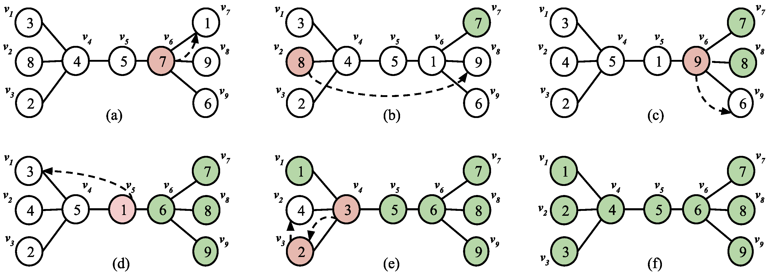
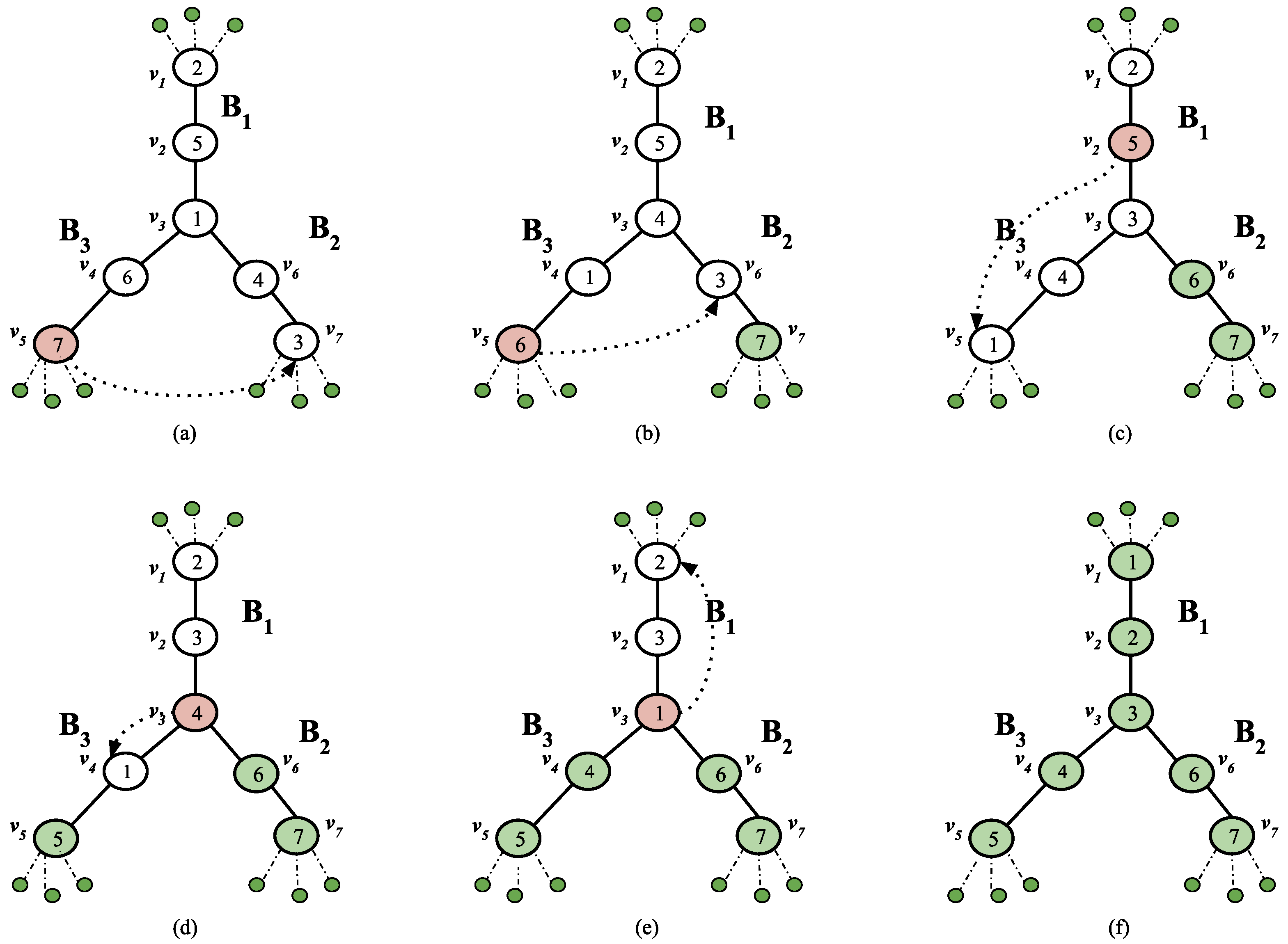
• Two star markers will never swap on a path edge.
  Proof. 

  Let us take x and y to be the star markers that swap on the path edge in S. We show how S can be modified to obtain a swap sequence with a lesser number of swaps on the path. After the swap of x and y in S, at some point of time, both x and y will get into the star. Let $S^{\prime }$ be a sub sequence of S, where y resides on a star leaf and x on the center node. To modify S, remove the swap of x and y and replace x with y and vice versa for the following swaps. Iterate this till the point $S^{\prime }$ is reached in S and add a swap of x and y. We have achieved the same target state, but a swap carried out on the path is removed and compensated by adding an additional swap in the star.    □
  To illustrate the same, consider the swap sequence $S=(1,2),(2,6),(2,3),(1,6),(1,3),$$(1,4)$. Note that $S^{\prime }=(1,2),(2,6),(2,3),(1,6),(1,3)$, where we have 2 at star leaf (say x) and 1 at the center (say y).
  If we omit the swap move (1, 2) and exchange $x=1$, $y=2$ we get the modified swap sequence as $(1,6),(1,3),(2,6),(2,3)$ (refer Figure 4). Followed by a swap move of x and y we achieve the same configuration as $S^{\prime }$ but the swap of x and y on path edge is replaced by a swap on star edge, resulting in lesser swaps on path edges.
• In every swap on the path edge involving at least one path marker, the larger of the markers will move to the right.
  Proof. 

  Considering the contradiction of the stated property, a bad swap involves moving a smaller valued path marker to the right and larger valued path marker to the left. Suppose S contains a bad swap. We show how S can be modified to obtain a new swap sequence which contains fewer swaps on the path. Assume smaller marker s is swapped to the right and larger marker l to the left. Property 1 restricts us from directly swapping them again. Therefore, marker l will move to the star leaf, then marker s to another star leaf and then l goes to the center of the star. Let us call this intermediate placement as $S^{\prime }$. Now, to modify S, remove the swap of s and l, and continue with the preceding swaps with s and l exchanged until the state $S^{\prime }$ is reached. We have achieved the same target state, but a swap carried out on the path is removed and compensated for by adding an additional swap in the star; hence, reducing the swap count on the path edge.    □
• No star marker moves past the first path edge from left to right.
  Proof. 

  Let S include a swap $S_i$ in which a maker x moves past the first path edge to the right using a swap with a marker p. Let, $S_j$ is a swap belonging to S where $j>i$ which results in x reentering the star with the help of a swap with q. Taking the least possible j into account, we first establish that the marker q was residing on the star leaf during $S_i$. Suppose q was on path node during $S_i$, then q will lie on the right to x. Swaps involving x between $S_i$ and $S_j$ will only keep it on path nodes and not move it past the first path edge as per our assumption. Marker q is restricted to swap twice with x on the path edge as per Property 1, which proves that q lies on the right of x during $S_j$, which is contradictory. We show how S can be modified to obtain a swap sequence with a lesser number of swaps on the path. Before $S_i$, carry out a swap of x and q and continue with the following swaps till $S_j-1$ with x replaced with y and vice-versa. We have achieved the same target state but the swap on a path edge is removed and replaced by a swap on a star edge, hence reducing the number of swaps on the path edge.    □

Theorem 1.

Algorithm $A_b$ computes an optimal swap sequence, i.e., a sorting sequence with the least possible number of swaps.

Proof. 

We prove that our algorithm obtains an optimal swap sequence by applying induction on marker n. The base case is just a star S. Depending on the position of $S_{min}$ and $P_{max}$, we consider different cases and prove them individually. Moreover, for the general induction step, we prove that swaps performed by $S_{min}$ and $P_{max}$ are a part of an optimal swap sequence.

Case (1): The initial position of $S_{min}$ is any path vertex other than the center vertex. Let $S_{opt}^{\prime }$ be the optimal swap sequence. Property 2 and Property 3 ensures that n will never encounter a star marker on the path and hence it will only swap path markers on its way home. Let d be the distance from the initial position of marker n to its home vertex $H_n$. So, $S_{opt}^{\prime }$ contains d swaps which involves marker n. Let $S_i$ be the swap that homes marker n, therefore $S_1,S_2,\dots ,S_i$ contain d swaps which includes marker n and $(i-d)$ swaps that do not include marker n. Call this intermediate configuration T. Create a separate swap sequence $S_{opt}$ which homes n in first d swaps followed by $i-d$ swaps that do not involve n and then carry on with rest of the swaps from $S_{i+1},\dots ,S_k$. Homing marker n does not alter the relative order of the remaining markers. Clearly, we have attained the same configuration state as in T, implying $S_{opt}$ is an optimal swap sequence which is generated by our algorithm $A_b$.

Consider $S^{\prime }$ be an optimal swap sequence which brings n to the center vertex. Observe that n can be placed on center in exactly $d-1$ swaps, where d is the distance of n from its home vertex $H_n$ on the star leaf. Let $S_c$ be the swap in $S^{\prime }=S_1,S_2,\dots ,S_c$ that places marker n on the center and T be the intermediate configuration of the markers after $S_c$. Create a swap sequence S that homes the marker n first in $d-1$ swaps and carries out the rest of the $c-(k-1)$ swaps, which does not include n. Clearly, you will get the same resulting configuration as of T with the same number of swaps. Hence, S is an optimal swap sequence.

Now, call $S_h$ the swap that homes n from the center vertex by swapping it with an arbitrary marker t residing on $H_n$. Aforementioned discussion assumes that no swaps which involve star edges occur before $S_h$. Otherwise, when n is initially placed on the center vertex or arrives at the center with the swap $S_c$, it suffices to show that $S_{opt}$ is optimal which does not alter the position of n before the swap $S_h$. We do some modifications in $S_{opt}$ to make this true. Split the subsequence $S_1,S_2,\dots ,S_{h-1}$ into $S_{path}$ and $S_{star}$, where the subsequence $S_{path}$ contains the swaps that occur on path edges and the subsequence $S_{star}$ contains the swaps that occur on star edges. Note that $S_{path}$ does not move marker n from its position and $S_{star}$ always places n back to the center. We can rearrange this subsequence containing $S_{star}$ and $S_{path}$ as there are no star markers moving towards the path and vice versa as mentioned in Property 5. After $S_{path}$, carry out the swap $S_h$ and then perform the swaps in $S_{star}$ but with t and n exchanged. This results in the same placement of markers with no change in the swap count on the star and path. Hence, $S_{opt}$ is same as the optimal sequence generated by our algorithm $A_b$.

Case (2): After Step 1 of $A_b$, it is important to observe that we are now only left with path markers as all the star markers are either homed or residing on star nodes (will be homed in Step 3). So, lets consider marker $n=P_{max}$ is on a path vertex, except the center vertex. According to the property proved before, $P_{max}$ will always move to the right, swapping the lesser value marker to the left. Let S be the swap sequence which contains swap moves for homing $P_{max}$. Consider $S_h$ to be the swap which slots $P_{max}$ in its home and T be the configuration at that instance. Considering distance d between $P_{max}$ and its home, we can say $S_1\dots S_h$ will have d swaps involving $P_{max}$ and $(i-d)$ not involving $P_{max}$ (say $S^{\prime }$ be that swap sequence). To modify S, we first make d swap moves which involve $P_{max}$, followed by $S^{\prime }$ and then $S_{i+1}\dots S_{final}$, call this swap sequence $S_o$. It is interesting to observe that initial d swap moves will not change the relative order of the rest of the path markers, post which, $S^{\prime }$ swap moves can be performed, ultimately resulting in the same configuration T; hence $S_o$ is optimal.

Now, suppose $n=P_{max}$ is on the center vertex. Let $S_p$ be the swap that marker n on the first path edge $e=(v_{k+1},v_{k+2})$ with an arbitrary marker t. If we assume there are no swaps before $S_p$, we can just prove it with the above mentioned discussion in Case 2. Else, it suffices to show that $S_{opt}$ is optimal and does not alter the position of n before $S_p$. We modify $S_{opt}$ to make this true. Split the subsequence $S_1,S_2,\dots ,S_{p-1}$ into $S_{path}$ and $S_{star}$, where $S_{path}$ contains the swaps that occur on path edges and $S_{star}$ contains the swaps that occur on star edges. Note that $S_{path}$ does not move marker n from its position and $S_{star}$ always places n back to the center. Additionally, as per Property 5 we can rearrange the subsequence containing $S_{star}$ and $S_{path}$ as there are no star markers moving towards the path and vice versa. To rearrange this subsequence, perform the swaps in $S_{path}$, then the swap $S_p$ followed by the swaps in $S_{star}$. While performing the saps in $S_{star}$ replace the marker n with marker t. This results in same placement of markers with no change in the swap count on the star and path edges; hence, $S_{opt}$ is optimal and is the same as the one generated by our algorithm $A_b$.

Case (3): As discussed before, for Step 3 the optimal number of swaps are $L_S+N_S$ where $L_S$ be the number of permutations that have a length ≥ 2 not involving the center vertex (say $V_c$) and $N_S$ be the number of markers that are in these permutations. In case of star, consider a sequence P of length ≥ 2 and the star vertices (say $V_s$). If $V_c\notin P$, then the total swap count to sort P is $V_s+1$. If $V_c\in P$, then the total swap count is $V_s$. As the cycles in $L_S$ are not related to each other, $L_S+N_S$ gives the optimal swap count.    □

4. Sorting Permutations with a Double Broom

A novel polynomial algorithm $A_{db}$ is designed in this section for optimally sorting permutations using a double broom. A double broom is a double star with their central vertices joined with a path (also known as a stem) [24]. Suppose double broom has a total of n vertices, $v_1,v_2,\dots ,v_i$ on the left star, $v_{i+1},\dots ,v_j$ residing on the path (or stem) and $v_{j+1},\dots ,v_n$ on the right star. Note that we consider the central vertices $v_{i+1}$ and $v_j$ of the stars as path vertices of the double broom.

Let $S_L$ and $S_R$ be the left and right stars respectively, with corresponding center vertices $C_L$ and $C_R$. Let $S_{min}^R$ and $S_{min}^L$ be the closest star marker residing on the path to $S_R$ and $S_L$ respectively and $P_{max}$ be the maximum valued unhomed path marker.

Our algorithm $A_{db}$, that transforms a given input configuration to a sorted configuration, is as follows:

• While ∃ a $S_{min}^R$ marker, efficiently home $S_{min}^R$;
• While ∃ a $S_{min}^L$ marker, efficiently home $S_{min}^L$;
• (At this point, only the stem is left) While ∃ a $P_{max}$ marker, efficiently home $P_{max}$;
• Efficiently home the markers of $S_R$ and $S_L$.

Note that any vertex to the right of $C_L$ (inclusive) will be considered as a path vertex from the perspective of a marker residing in $S_L$. Similarly, any marker to the left of $C_R$ (including) will be a path vertex for markers in $S_R$.

Our algorithm places each marker at its respective vertex in 10 swaps (refer Figure 5). It is also noteworthy to mention that the happy leaves are swapped in the process, hence abiding to the Happy Leaves conjecture. $A_{db}$ obeys following interesting properties which we use to analyse the algorithm in the next section.

• Swap of two star markers belonging to a same star will never take place on a path edge;
• Stem marker moves right to its home, swapping smaller markers to the left.

4.1. Analysis of $A_{db}$

Let $T_{db}$ be the total number of swaps performed in $A_{db}$. We first consider step 4 of our algorithm. For $S_L$, let $C_{NT}^{S^L}$ be the non trivial cycles and $n_S{S}_L$ be the number of markers in these cycles. Similarly, for $S_R$, let $C_{NT}^{S_R}$ be the non trivial cycles and $n_S^{S_R}$ be the number of markers in these cycles. As these markers retain their relative positions till Step 4 of our algorithm, our total number of swaps $T_{S_R,S_L}$ in Step 4 will be:

$$T{}_{S{}_R,S{}_L}=C_{NT}^{S_L}+n_S^{S_L}+C_{NT}^{S_R}+n_S^{S_R}.$$

Let $T_R$ and $T_L$ be the total number of swaps carried out in Step 1 and Step 2 respectively. To analyse $T_R$ and $T_L$, we allocate each of its swaps to closest star marker residing on the path and involved in the swap. Then,

$$T{}_R=\sum _{S{}_{min}^R}T\left(S{}_{min}^R\right),$$

where $T\left(S_{min}^R\right)$ is the number of swaps allocated to closest star marker $S_{min}^R$. For $S_{min}^R$, define $D\left(S_{min}^R\right)$ to be the distance from a star leaf to $S_{min}^R$’s home. With reference to the initial configuration state of the markers, let $R\left(S_{min}^R\right)$ be the number of markers smaller than $S_{min}^R$ and on the right of $S_{min}^R$.

$$T{}_L=\sum _{S{}_{min}^L}T\left(S{}_{min}^L\right).$$

Similarly, for $S_{min}^L$, define $D\left(S_{min}^L\right)$ to be the distance from a star leaf to $S_{min}^L$’s home and let $L\left(S_{min}^R\right)$ be the number of markers greater than $S_{min}^L$ and on the right of $S_{min}^L$.

Claim 1. 

$T\left(S_{min}^R\right)$is the minimum of$D\left(S_{min}^R\right)$and$R\left(S_{min}^R\right).$

Proof. 

If $T\left(S_{min}^R\right)$ or $S_{min}^L$ are at star leaf of $S_L$ or $S_R$ respectively in the current configuration of markers, we can say $T\left(S_{min}^R\right)$ = $D\left(S_{min}^R\right)$ implying $D\left(S_{min}^R\right)\le R\left(S_{min}^R\right)$. $T\left(S_{min}^R\right)$ = $D\left(S_{min}^R\right)$, where $D\left(S_{min}^L\right)\le L\left(S_{min}^L\right)$ and thus validating our claims.    □

Claim 2. 

$T\left(S_{min}^L\right)$is the minimum of$D\left(S_{min}^L\right)$and$L\left(S_{min}^L\right)$.

Proof. 

If $S_{min}^R$ is not at a star leaf of $S_L$, we can say $R\left(S_{min}^R\right)<D\left(S_{min}^L\right)$. Similarly, in case of $S_{min}^L,L\left(S_{min}^L\right)<D\left(S_{min}^L\right)$, justifying the above mentioned claims.    □

Claim 3. 

In algorithm$A_{db}$, swapping Steps 1 and 2 does not alter the swap count.

Proof. 

In the initial configuration, let $S_{L\to R}$ and $S_{P\to R}$ to be the number of star markers residing in $S_L$ and on the path, respectively, whose homes are in $S_R$. Similarly, let $S_{R\to L}$ and $S_{P\to L}$ be the number of star markers residing in $S_R$ and on the path respectively whose homes are in $S_L$. Path markers can be in $S_L$, $S_R$, or on the path. Let the total swaps required for homing path markers be $P=P_P+P_R+P_L$, where $P_P$, $P_R$, and let $P_L$ be the swap count for homing markers residing on the path, $S_R$ and $S_L$ respectively.

Case (1): Perform Step 1 of $A_{db}$ followed by Step 2. Moving $S_{min}^R$ towards the right, shifts the markers it encounters on the way to the left. This shift decreases $S_{R\to L}$ and $S_{P\to L}$. Path markers entering into $S_L$ (say $P_L^{\prime }$) during a swap increase P and the number of path tokens leaving $S_R$, i.e., $P_R$ will result in the decrease of P.

$$T_R+(T_L-(S_{R\to L}+k))+(P+P_L^{\prime }-P_R),\mathrm{where}0\le k\le S_{P\to R}.$$

(1)

In Step 2, $S_{min}^L$ can encounter only path markers on the way home. $S_{min}^L$ shifts both $P_L^{\prime }$ markers which entered into $S_L$ in Step 1 and $P_L$ markers to the right.

$$(T_L-(S_{R\to L}+k))+((P+P_L^{\prime }-P_R)-(P_L^{\prime }+P_L)).$$

(2)

At this point, we are now left only with $P_P$ as all the path markers are now residing on the path, for which the swap count will be the total number of inversions.

Case (2): Perform Step 2 of $A_{db}$ followed by Step 1. Moving $S_{min}^L$ towards the left, shifts the markers it encounters on the way to the right. This shift decreases $S_{L\to R}$ and $S_{P\to R}$. Path markers entering into $S_R$ (say $P_R^{\prime }$) during a swap increase P and the number of path tokens leaving $S_L$ i.e., $P_L$ will result in the decrease of P.

$$T_L+(T_R-(S_{L\to R}+k))+(P+P_R^{\prime }-P_L),\mathrm{where}0\le k\le S_{P\to L}.$$

(3)

In Step 2, $S_{min}^R$ can encounter only path markers on the way home. $S_{min}^R$ shifts both $P_R^{\prime }$ markers which entered into $S_R$ in Step 1 and $P_R$ markers to the left.

$$(T_R-(S_{L\to R}+k))+((P+P_R^{\prime }-P_L)-(P_R^{\prime }+P_R)).$$

(4)

At this point, we are now left only with $P_P$, the same as what we arrived at in Case 1. Markers traversing towards $S_R$ in Step 1 of $A_{db}$ shift all the markers whose home is in $S_L$ to the left. Similarly, markers traversing towards $S_L$ shift all markers to the right; hence, there are no bad swaps and the properties of $A_{db}$ are obeyed.    □

In Step 3, observe that we are now left only with the stem markers. The total number of swaps on path are the same as the number of inversions required to place the markers at their desirable vertex. Let $D\left(P_{max}\right)$ be the distance from the marker $P_{max}$ to its home. Similarly, we can say:

$$T{}_{P_{max}}=\sum _{P{}_{max}}D\left(P{}_{max}\right),$$

where $T_{P_{max}}$ are the total number of swaps in Step 3 and $P{}_{max}$ are the markers residing on the stem of the broom.

Lemma 2.

$$T{}_{db}=T{}_{S{}_R,S{}_L}+T\left(S{}_{min}^R\right)+T\left(S{}_{min}^L\right)+\sum _{P{}_{max}}D\left(P{}_{max}\right).$$

Similar to algorithm $A_b$, time complexity of $A_{db}$ is also expressed in terms of the number of moves. The worst case of Step 1 occurs when all path vertices are occupied by star markers of $S_R$ and the homes of these star markers are occupied by other $S_R$ markers. The total number of moves required in this case is $(P(P+1)/2)+\left(S_{L->R}\right)\ast (P+1)+(S_1-P)$, where $S_1$ and P are the number of vertices in $S_R$ and path respectively. The worst case of Step 2 occurs when all the path vertices are occupied by star markers of $S_L$ and the homes of these star markers are occupied by other $S_L$ markers. The total number of moves required in this case is $(P(P+1)/2)+(S_2-P)$, where $S_2$ is the number of vertices in $S_L$. In the worst case of Step 3, $P(P-1)/2$ moves are required to home the P path markers. Step 4 requires $\lfloor 3S_1/2\rfloor +\lfloor 3S_2/2\rfloor$ moves at most. Since $P,S\in O\left(n\right)$, Algorithm $A_{db}$ runs in $O\left(n^2\right)$ time. The tree requires $O\left(n\right)$ space, and the algorithm does not require any additional space.

4.2. Correctness of $A{}_{db}$

In this section, we prove that our algorithm $A_{db}$ generates an optimal swap sequence on a double broom. Initially, we discuss some properties required to prove the correctness of our algorithm. Section 1 covers the proof for properties 1 to 5.

• Two same markers will not swap more than once;
• Star markers belonging to the respective star enter into the star in the increasing order of their distances from that star;
• Star markers belonging to the respective star never swap with each other on the path edges. Note that the star marker belonging to $S_L$ treats the edges of the $S_R$ as path edges and vice-versa;
• Swaps on the stem involving at least one stem marker—the larger of the markers will move to the right’
• No star marker residing on one if its star vertices moves past the first path edge;
• In a swap s = ($l,r$) where $l\in S_L$ and $r\in S_R$, l always moves to the left and r to the right.

Proof 

We prove it by contradiction. A $badswap$ involves moving l to the right and r to the left. Suppose S has a $badswap$ on the path. We show how S can be modified to obtain a new swap sequence which contains fewer swaps on the path. Property 1 restricts us from directly swapping them again. Therefore, marker r will move to the star leaf of $S_L$ (or l will move to the star leaf of $S_R$), then marker l to another star leaf of $S_L$ (or r will move to another star leaf of $S_R$) and then l goes to the center of $S_l$ (or r will move to the center of $S_R$). Let us call this intermediate placement of markers $S^{\prime }$. To modify S, omit the swap of l and r, and carry on with the preceding swaps with l and r exchanged until the state $S^{\prime }$ is reached. This results in the same swap count, though a swap on star replaces a swap on path.    □

Theorem 2.

Algorithm $A_{db}$ generates an optimal swap sequence, i.e., a sorting sequence with the least possible number of swaps.

Proof. 

We prove that our algorithm obtains an optimal swap sequence by applying induction on marker n. For the base case, the double broom has no path edges and it is only a star (either $S_R$ or $S_L$). It is interesting to note that, this algorithm $A_{db}$ is equivalent to writing:

• While ∃ a $S_{min}^R$ marker, home $S_{min}^R$.
• Run $A_{db}$
• Solve $S_R$

As discussed in the previous section, $A_b$ obtains an optimal solution and we are now left to prove only in case of $S_{min}^R$. Depending on the position of $S_{min}^R$, we consider different cases and prove them individually. In the general induction step, we prove that swaps performed by $S_{min}^R$ are part of the optimal swap sequence.

Case (1): Assume marker n = $S_{min}^R$ is initially placed on a stem vertex, except the center node of $S_R$. Let $P_{opt}^{\prime }$ be the optimal swap sequence. Property 2 and Property 3 ensures that n will never swap with a star marker on its way home in $S_R$. Let d be the distance from the position of marker n to its home $H_n$. So, there are exactly d swaps in $P_{opt}^{\prime }$ which contain marker n. Let $S_i$ be the swap that homes marker n, therefore $S_1$, $S_2,\dots ,S_i$ contain d swaps which includes marker n and $(i-d)$ swaps that do not include marker n. Let this intermediate configuration be T. Create a separate swap sequence $P_{opt}$ which takes the initial d swaps to homes n, followed by $i-d$ swaps that do not involve n and then carry on with rest of the swaps from $S_{i+1},\dots ,S_k$. Initial d swaps leave the remaining markers in the same relative order. We have attained the same configuration state as in T implying the swap sequence $P_{opt}$ is optimal and is same as the one generated by our algorithm $A_{db}$.

Case (2): Consider $S^{\prime }$ be an optimal swap sequence which brings n to the center vertex. Observe that n can be placed on center in exactly $d-1$ swaps, where d is the distance of n from its home vertex $H_n$ on the star leaf. Let $S_c$ be the swap in $S^{\prime }=S_1,S_2,\dots ,S_c$ that places marker n on the center and T be the intermediate configuration of the markers after $S_c$. Create a swap sequence S that homes n first in $d-1$ swaps and carries out the rest of the $c-(k-1)$ swaps which does not include n. Clearly, you will get the same resulting configuration as of T with the same number of swaps. Hence, S is an optimal swap sequence.

Now, call $S_h$ the swap that homes n from the center vertex of $S_R$ by swapping it with an arbitrary marker t residing on $H_n$. Previous discussion assumes that no swaps occur on the star edges before $S_h$. Otherwise, when n is initially placed on the center vertex or arrives at the center with the swap $S_c$ it suffices to show that $S_{opt}$ is optimal and does not alter the position of n before the swap $S_h$. We do some modifications in $S_{opt}$ to make this true. Split the subsequence $S_1,S_2,\dots ,S_{h-1}$ into two subsequences $S_{path}$ and $S_{star}$. $S_{path}$ contains the swaps that occurs on path edges and $S_{star}$ contains the swaps that occurs on star edges. Note that $S_{path}$ does not move marker n from its position and $S_{star}$ always places n back to the center. We can rearrange this subsequence containing $S_{star}$ and $S_{path}$ as no star markers move towards the path and vice versa, due to the aforementioned Property 5. After $S_{path}$, carry out the swap $S_h$ and then perform the swaps in $S_{star}$ but with t in place of n. Note that we can use the same argument for n placed on $S_L$ and prove the optimality of the subsequence as in Case 1. Clearly, this gives the same placement of markers with same swap count on the star and path. Hence, $S_{opt}$ is optimal and is same as the sequence generated by our algorithm $A_{db}$.

Case (3): Assume $n=S_{min}^R$ is on the leaf vertex of $S_L$. Let t be the marker on the center vertex and $S_h$ be the swap involving n and t. If there are no swaps before $S_h$, then just perform $S_h$ and use the argument from Case 2 to prove the optimality of the sequence $P_{opt}$. Otherwise, suppose there exists a cyclic permutation $P_s$ of length $L_s-1$ for the markers residing in $S_L$. Cycles which do not include n are not taken into consideration, as solving those cycles will not alter the position of n. Similar to the argument used for star, we prove that the $P_s$ can be solved in $L_s$ swaps. Each marker in C is far away by two swaps from its home, so the total distance is $2(L_s-1)$. However, as one swap helps us move two markers near to their respective homes, our requirement is only $L_s-1$ swaps. Interestingly, the initial and the final swap of $P_s$ moves only one marker which belongs to $P_s$. Adding the swap of n and t results in a total of $L_s+1$ swaps contradictory to $L_s-1$ swaps to sort $P_s$.    □

5. Analysis of Algorithm D* on Millipede Tree

The first known upper bound $f\left(\mathsf{\Gamma }\right)$, for sorting permutations using transposition trees, was computed by Akers and Krishnamurthy [1] in 1989. The time complexity for calculating $f\left(\mathsf{\Gamma }\right)$ is $\mathsf{\Omega }(n!n^2)$, since it performs pair wise distance computation of each of the possible $n!$ permutations. Subsequently, various polynomial time approximation algorithms were designed [23,24,25,29,30]. Chitturi introduced algorithm $D^{\prime }$ in [24] which finds the upper bound ${\delta }^{\prime }$ in polynomial time, which is the tightest known upper bound when the upper bounds of all trees are summed together. Subsequently, algorithm $D^{*}$ which identifies corresponding the upper bound ${\delta }^{*}$ was designed in [29]. It was shown that ${\delta }^{*}$ is tighter for balanced-starburst tree [29]. In [31], an analysis of both $D^{\prime }$ and $D^{*}$ was performed and shows that ${\delta }^{*}$ is tighter for full binary tree too. In this section we define a class of trees called millipede tree for which ${\delta }^{*}$ is tighter, compared to ${\delta }^{\prime }$.

A millipede tree $M_k$ is obtained by connecting the centre vertices $c_1,c_2,\dots c_k$ of k path graphs $p_1,p_2,\dots p_k$ arranged in the order, such that k is odd and the number of vertices in $p_i$ is given by the following function:

$$n\left(p_i\right)=\left\{\begin{array}{cc}2i+1\hfill & \mathrm{if}1\le i\le \lceil k/2\rceil \hfill \\ 2(k-i)+3\hfill & \mathrm{Otherwise}.\hfill \end{array}\right.$$

(5)

The diameter of $M_k$ is $(k+1)$ and the total number of vertices $n=2\ast [\lceil k/2\rceil$$\ast (\lceil k/2\rceil +1)]-1$. $v_c=c_{(k+1)/2}$ is the center of the tree. The center has an eccentricity of $(k+1)/2$.

We call the subtree above the vertex $v_c$ the upper millipede tree and the subtree below $v_c$ the lower millipede tree(refer Figure 6).

5.1. Algorithm $D^{*}$

Throughout this section, we employ the terminology used in [1,24,29]. The eccentricity of a node u in $V_T$, denoted by $ecc\left(u\right)$, is equal to the maximum value of the distance between u and any other node $v\in V_T$. The Center of a tree is a node with minimum eccentricity. The Diameter of T denoted as $diam\left(T\right)$ is the maximum among all the eccentricities. The set of vertices in $V_T$ with maximum eccentricity is defined as S. S is a subset of the leaf nodes. Algorithm $D^{\prime }$ deletes a set of leaf nodes $L\subset V_T$, and calculates the upper bound required to home markers destined to the vertices in L. This process is continued till the graph becomes a star. The exact upper bound for a star is defined in [1], which is $\lfloor 3(n-1)/2\rfloor$. Let S be divided into kclusters $C_1,C_2,\cdots C_k$ such that for any $u,v$ in $C_i$, ${\forall }_{i=1\cdots k}{d}_T(u,v)<diam\left(T\right)$. Let X be any one of the k clusters. When the vertices of $S\setminus X$ are deleted, then the diameter of the resultant tree decreases by one. The maximum distance a marker need to travel to be homed is the diameter of the tree, $diam\left(T\right)$. Thus, $D^{\prime }$ deletes all the vertices of S, except the largest cluster $C^{*}$, so that minimum number of markers are homed at the current diameter and then reduces the diameter by one. Since the markers homed to the leaves are not required to move further, algorithm $D^{\prime }$ deletes such leaves from the tree. Two variants of $D^{\prime }$, named $D_{v1}^{\prime }$ and $D_{v2}^{\prime }$ were introduced. $D_{v1}^{\prime }$ removes the entire set S if $\left|C\right|>\frac{2}{3}\left|S\right|$ and $D_{v2}^{\prime }$ removes S if $\left|C\right|\ge \frac{2}{3}\left|S\right|$, where $C=S\setminus C^{*}$. $D^{*}$, which calculates the upper bound ${\delta }^{*}$ [29] is an improved version of $D^{\prime }$. If $|S\setminus C^{*}|>|C^{*}|$, then at most $|C^{*}|$ markers need $diam\left(T\right)$ moves each to be homed. Algorithm $D^{*}$ works based on this idea. The proof can be seen in [29,31]. $D^{*}$ deletes $|C^{*}|$ nodes in $diam\left(T\right)$ cost and the remaining nodes in the cluster with $\left(diam\right(T)-1/2)$ cost. It is observed that the ${\delta }^{*}$ is tighter than ${\delta }^{\prime }$ when $|C^{*}|$ is between one-third and half of the total size of set $\left|S\right|$.

5.2. Analysis and Results

It is observed that $D^{*}$ would yield a tighter upper bound than $D^{\prime }$ for a millipede tree. In the first iteration of $D^{*}$ on $M_k$, the set S contains all the leaf nodes and results in two clusters—$C_1$ and $C_2$. $C_1$ and $C_4$ are of same size which contain the leaf nodes in the upper and lower millipede trees respectively (refer Figure 7). The terminal nodes in the path graph $p_{(k+1)/2}$ are not part of any cluster. Note that, deleting $C_1$ or $C_2$ will result in isomorphic trees (refer Figure 8). Since the size of the largest cluster $C^{*}$ ($C_1$ or $C_2$) is less than half of the size of S, only $|C^{*}|$ markers need to be homed in $diam\left(T\right)$ cost and the remaining markers in the set S can be homed at a cost of $\left(diam\right(T)-1/2)$. This results in two steps $x_1$ and $x_2$ for calculating the total cost in the iteration:

${\mathbf{x}}_{\mathbf{1}}$: ${\delta }^{*}=diam\left(T\right)\ast \left|C^{*}\right|$

; ${\mathbf{x}}_{\mathbf{2}}$: ${\delta }^{*}=(diam\left(T\right)-1/2)\ast |C-C^{*}|$.

Algorithm 1 Algorithm $D^{*}$ [29]

1: ${\delta }^{*}\leftarrow 0$   2: ifT is a star then   3:     ${\delta }^{*}\leftarrow {\delta }^{*}+\lfloor 3/2\left(\right|V_T|-1)\rfloor$ and terminate.   4: end if   5: Identify S, the set of vertices with maximum eccentricity.   6: Compute clusters for S.   7: Identify $C=S-C^{*}$ where $|C^{*}|$ is the max. If there are multiple such clusters, choose the one with minimum distance sum.   8: Case 1: $|C^{*}|\ge |S|/2$   9: ${\delta }^{*}\leftarrow {\delta }^{*}+\left|C\right|\ast diam\left(T\right)$$T\leftarrow T\setminus V_C$ 10: End Case 1 11: Case 2: $|C^{*}|<|S|/2$ //$\left|C\right|\ge |C^{*}|$ 12: ${\delta }^{*}\leftarrow {\delta }^{*}+\left|C^{*}\right|\ast diam\left(T\right);T\leftarrow T\setminus V_C$ 13: if$\left|C\right|-|C*|$ is even then 14:     ${\delta }^{*}\leftarrow {\delta }^{*}+\left(\right|C|-|C^{*}\left|\right)\ast (diam\left(T\right)-1/2)$; 15: else 16:     ${\delta }^{*}\leftarrow {\delta }^{*}+\left(\right|C|-|C^{*}\left|\right)\ast (diam\left(T\right)-1/2)-1/2$; 17: end if 18: End Case 2 19: ifT is not a star graph then go to step 5. 20: else 21:     ${\delta }^{*}\leftarrow {\delta }^{*}+\lfloor 3/2\left(\right|V_T|-1)\rfloor$ and terminate. 22: end if

In the case of $D^{\prime }$, there is only one step and all the markers of C are homed in $diam\left(T\right)$ cost. Two nodes are homed in Step ${\mathrm{x}}_2$ resulting in an improvement of 1 in ${\delta }^{*}$. As $D^{*}$ and $D^{\prime }$ delete all the vertices of $S\setminus C^{*}$, the resultant tree after the first iteration is same for both. Similarly, every odd iteration generate two clusters and result in an improvement of 1. The second iteration generates two clusters $C_1$ and $C_2$, which contain the leaf nodes of the upper and lower millipede trees respectively. Even iterations do not result in any improvement in ${\delta }^{*}$, as both the algorithms remove $\left|C\right|$ nodes in $diam\left(T\right)$ cost. Refer

Table 1. Cost of removing nodes in $D{}^{\prime }$ and $D^{*}$ on millipede tree.

Iteration	${\mathit{C}}^{*}$	$\mathit{S}-{\mathit{C}}^{*}$	$\mathit{D}{}^{\prime }\mathit{C}\left({\mathit{C}}^{*}\right)$	$\mathit{D}{}^{\prime }\mathit{C}(\mathit{S}-{\mathit{C}}^{*})$	${\mathit{D}}^{*}\mathit{C}\left({\mathit{C}}^{*}\right)$	${\mathit{D}}^{*}\mathit{C}{(\mathit{S}-{\mathit{C}}^{*})}^{*}$
1	(k − 1)	2	d	d	d	(d − 1/2)
2	k	1	(d − 1)	(d − 1)	(d − 1)	-
3	(k − 2)	2	(d − 2)	(d − 2)	(d − 2)	(d − 2 − 1/2)
4	(k − 2)	0	(d − 3)	-	(d − 3)	-
5	(k − 4)	2	(d − 4)	(d − 4)	(d − 4)	(d − 4 − 1/2)
6	(k − 4)	0	(d − 5)	-	(d − 5)	-
7	(k − 6)	2	(d − 6)	(d − 6)	(d − 6)	(d − 6 − 1/2)
8	(k − 6)	0	(d − 7)	-	(d − 7)	-
…	…	…	…	…	…	…
(k − 1)	3	0	3	-	3	-

, where $D^{\prime }C\left(C^{*}\right)$ is the cost per node for homing $|C^{*}|$ nodes in Algorithm $D^{\prime }$, $D^{\prime }C(S-C^{*})$ is the cost per node for homing $|S\setminus C^{*}|$ nodes in Algorithm $D^{\prime }$, $D^{*}C\left(C^{*}\right)$ is the cost per node for homing $|C^{*}|$ nodes in Algorithm $D^{*}$ and $D^{*}C(S-C^{*})$ is the cost per node for homing $|S\setminus C^{*}|$ nodes in Algorithm $D^{*}$. After $(k-1)$ iterations in $M_k$, the tree becomes a star, which is the base case of both the algorithms.

As mentioned above, $D^{*}{C}_o=D{}^{\prime }{C}_o-1$ where $D{}^{\prime }{C}_o$ is the cost computed in $D^{\prime }$ and $D^{*}{C}_o$ is the cost computed in $D^{*}$, for every odd iteration. Therefore after the ith iteration, the total improvement is $\lceil (i+1)/2\rceil$.

The upper bound value for all millipede trees with diameters up to 16 was computed for both $D^{\prime }$ and $D^{*}$. The results (refer

Table 2. Comparison of ${\delta }^{\prime }$ and ${\delta }^{*}$ on millipede trees with various diameters.

Tree	Diameter	No:of Nodes	${\mathit{\delta }}_{\mathit{v}1}^{\prime }$	${\mathit{\delta }}_{\mathit{v}2}^{\prime }$	${\mathit{\delta }}^{*}$	${\mathit{\delta }}^{\prime }-{\mathit{\delta }}^{*}$
$M_3$	4	11	28	28	27	1
$M_5$	6	23	92	92	90	2
$M_7$	8	39	209	209	206	3
$M_9$	10	59	396	396	392	4
$M_{11}$	12	83	669	669	664	5
$M_{13}$	14	111	1044	1044	1038	6
$M_{15}$	16	143	1537	1537	1530	7

) show that, ${\delta }^{*}$ is smaller than ${\delta }^{\prime }$. ${\delta }^{*}$ and ${\delta }^{\prime }$ are deterministic for a millipede tree since the choice of vertices for deletion in each iteration does not alter the upper bound. ${\delta }^{\prime }-{\delta }^{*}=(d/2)-1$ establishes the fact that ${\delta }^{*}$ is tighter on a millipede tree as the difference is directly proportional to the initial diameter d. In terms of the number of path graphs k in the tree $M_k$, ${\delta }^{\prime }-{\delta }^{*}$ can also be written as $\lfloor k/2\rfloor$.

Theorem 3.

${\delta }^{\prime }-{\delta }^{*}=\mathsf{\Omega }\left(k\right)$ for a millipede tree $M_k$.

6. Scope for Future Research

An n-Broom (where n ≥ 3) is a transposition tree where the terminal node of the paths of n single brooms are connected to a common node. Figure 9 shows one of the possible 4-Brooms. Figure 10 and Figure 11 show two different possible swap sequences for a 3-Broom, where brooms $B_1$, $B_2$ and $B_3$ are connected to the common node $V_3$. Assume that all the star markers are homed, and only the path markers are left to be homed. The figures do not show the star markers, since these markers need not be swapped while homing the path markers. Figure 10 and Figure 11 n-Broom impacts the total swap count. Homing the path markers in $B_3$ before the path markers in $B_1$ (Figure 11) resulted in a non-optimal swap sequence which required more swaps than the swaps executed in Figure 10. Hence, $A_{db}$ does not guarantee an optimal swap sequence for an n-broom. Thus, designing a polynomial time optimal algorithm for sorting permutations on n-brooms is open.

7. Conclusions

Sorting permutations using various operations has applications in computer interconnection networks and evolutionary biology. We designed a simpler $O\left(n^2\right)$ time algorithm for sorting permutations using the transposition tree single broom. We designed a novel $O\left(n^2\right)$ time algorithm for optimally sorting permutations with a double broom and proved its correctness.

We defined a new class of trees that we call millipede. Among the existing generic algorithms that sort with any given transposition tree, ${\delta }^{*}$ and ${\delta }^{\prime }$ are the tightest and are comparable to one another. We showed that ${\delta }^{*}$ yields a tighter upper bound than ${\delta }^{\prime }$ for a balanced millipede tree.

We also demonstrated how algorithm $A_{db}$ does not yield an optimal swap sequence in the case of n-Broom, concluding that a polynomial-time algorithm for n-broom can be a subject of future research.

References

1. Akers, S.B.; Krishnamurthy, B. A group-theoretic model for symmetric interconnection networks. IEEE Trans. Comput. 1989, 38, 555–566. [Google Scholar] [CrossRef]
2. Chitturi, B. On Transforming Sequences. University of Texas at Dallas. 2007. Available online: https://www.researchgate.net/profile/Bhadrachalam-Chitturi/publication/308524758_ON_TRANSFORMING_SEQUENCES/links/57e64be408aed7fe4667bb11/ON-TRANSFORMING-SEQUENCES.pdf (accessed on 1 June 2017).
3. Heydemann, M.-C. Cayley graphs and interconnection networks. In Graph Symmetry; Springer: Dordrecht, The Netherlands, 1997; pp. 167–224. [Google Scholar]
4. Lakshmivarahan, S.; Jwo, J.-S.; Dhall, S.K. Symmetry in interconnection networks based on Cayley graphs of permutation groups: A survey. Parallel Comput. 1993, 19, 361–407. [Google Scholar] [CrossRef]
5. Jain, B.A.; Lubiw, K.; Masárová, A.; Miltzow, Z.; Mondal, T.; Naredl, D.; Murty, A.; Josef, T.; Alexi, T. Token Swapping on Trees. arXiv 2019, arXiv:1903.06981. [Google Scholar]
6. Yamanaka, K.; Demaine, E.D.; Ito, T.; Kawahara, J.; Kiyomi, M.; Okamoto, Y.; Saitoh, T.; Suzuki, A.; Uchizawa, K.; Uno, T. Swapping labeled tokens on graphs. Theor. Comput. Sci. 2015, 586, 81–94. [Google Scholar] [CrossRef]
7. Cooperman, G.; Finkelstein, L. New methods for using Cayley graphs in interconnection networks. Discret. Appl. Math. 1992, 37–38, 95–118. [Google Scholar] [CrossRef]
8. Xu, J. Topological Structure and Analysis of Interconnection Networks; Springer Science & Business Media: Berlin/Heidelberg, Germany, 2013; Volume 7. [Google Scholar]
9. Knuth, D.E. The Art of Computer Programming: Sorting and Searching, 2nd ed.; Pearson Education: London, UK, 1997; pp. 426–458. [Google Scholar]
10. Vaughan, T.P. Factoring a permutation on a broom. J. Comb. Math. Comb. Comput. 1999, 30, 129–148. [Google Scholar]
11. Kawahara, J.; Saitoh, T.; Yoshinaka, R. The Time Complexity of the Token Swapping Problem and Its Parallel Variants. Walcom Algorithms Comput. 2017, 448–459. [Google Scholar]
12. Jerrum, M.R. The complexity of finding minimum-length generator sequences. Theor. Comput. Sci. 1985, 36, 265–289. [Google Scholar] [CrossRef] [Green Version]
13. Christie, D.A. Genome Rearrangement Problems; The University of Glasgow: Glasgow, UK, 1998. [Google Scholar]
14. Chitturi, B.; Das, P. Sorting permutations with transpositions in O(n3) amortized time. Theor. Comput. Sci. 2019, 766, 30–37. [Google Scholar] [CrossRef]
15. Chitturi, B. Computing cardinalities of subsets of Sn with k adjacencies. JCMCC 2020, 113, 183–195. [Google Scholar]
16. Malavika, J.; Scaria, S.; Indulekha, T.S. On Token Swapping in Labeled Tree. In Proceedings of the 2021 Third International Conference on Inventive Research in Computing Applications (ICIRCA), Coimbatore, India, 2–4 September 2021; pp. 940–945. [Google Scholar]
17. Bonnet, É.; Miltzow, T.; Rzazewski, P. Complexity of Token Swapping and Its Variants. Algorithmica 2017, 80, 2656–2682. [Google Scholar] [CrossRef] [Green Version]
18. Kawahara, J.; Saitoh, T.; Yoshinaka, R. The Time Complexity of Permutation Routing via Matching, Token Swapping and a Variant. JGAA 2019, 23, 29–70. [Google Scholar] [CrossRef]
19. Miltzow, T.; Narins, L.; Okamoto, Y.; Rote, G.; Thomas, A.; Uno, T. Approximation and hardness of token swapping. In Proceedings of the 24th Annual European Symposium on Algorithms (ESA 2016), Aarhus, Denmark, 22–24 August 2016; Volume 57. [Google Scholar]
20. Cayley, A. LXXVII. Note on the theory of permutations. Lond. Edinb. Dublin Philos. Mag. J. Sci. 1849, 34, 527–529. [Google Scholar] [CrossRef] [Green Version]
21. Pak, I. Reduced decompositions of permutations in terms of star transpositions, generalized catalan numbers and k-ARY trees. Discrete Math. 1999, 204, 329–335. [Google Scholar] [CrossRef] [Green Version]
22. Portier, F.J.; Vaughan, T.P. Whitney Numbers of the Second Kind for the Star Poset. Eur. J. Comb. 1990, 11, 277–288. [Google Scholar] [CrossRef] [Green Version]
23. Ganesan, A. An efficient algorithm for the diameter of cayley graphs generated by transposition trees. Aeng Int. J. Appl. Math. 2012, 42, 214–223. [Google Scholar]
24. Chitturi, B. Upper Bounds For Sorting Permutations With A Transposition Tree. Discret. Math. Algorithm. Appl. 2013, 5, 1350003. [Google Scholar] [CrossRef]
25. Kraft, B. Diameters of Cayley graphs generated by transposition trees. Discret. Appl. Math. 2015, 184, 178–188. [Google Scholar] [CrossRef]
26. Uthan, S.; Chitturi, B. Bounding the diameter of Cayley graphs generated by specific transposition trees. In Proceedings of the International Conference on Advances in Computing, Communications and Informatics (ICACCI), Udupi, India, 13–16 September 2017; pp. 1242–1248. [Google Scholar]
27. Balcza, L. On inversions and cycles in permutations. Period. Polytech. Civ. Eng. 1992, 36, 369–374. [Google Scholar]
28. Edelman, P.H. On Inversions and Cycles in Permutations. Eur. J. Comb. 1987, 8, 269–279. [Google Scholar] [CrossRef] [Green Version]
29. Chitturi, B.; Indulekha, T.S. Sorting permutations with a transposition tree. In Proceedings of the 8th International Conference on Modeling Simulation and Applied Optimization (ICMSAO), Manama, Bahrain, 15–17 April 2019. [Google Scholar]
30. Das, D.K.; Chitturi, B.; Kuppili, S.S. An Upper Bound For Sorting Permutations With A Transposition Tree. Procedia Comput. Sci. 2020, 171, 72–80. [Google Scholar] [CrossRef]
31. Indulekha, T.S.; Chitturi, B. Analysis of Algorithm δ* on full binary trees. In Proceedings of the 2019 Second International Conference on Advanced Computational and Communication Paradigms (ICACCP), Gangtok, India, 25–28 February 2019; pp. 1–5. [Google Scholar]
Figure 1. A Transposition tree T and the corresponding Cayley graph Γ T .
Algorithms 15 00220 g001
Figure 2. Illustration for Algorithm A b . The star vertices are v 1 , v 2 , v 3 , v 4 , v 5 and the path vertices are v 6 , v 7 , v 8 . (a) (i) S m i n = 3, Swaps = 2; (ii) S m i n = 2, Swaps = 3. (b) P m a x = 8, Swaps = 1. (c) Unhomed Markers are 5 and 4, Swaps = 3.
Algorithms 15 00220 g002
Figure 3. Comparison of algorithm A b with Biniaz’s and Kawahara’s algorithms. (a) S m i n = 3, Swaps = 2; S m i n = 4, Swaps = 3. (b) Maximum valued path token ( P m a x ) = 9, Swaps = 3; P m a x = 8, Swaps = 3. (c) Maximum valued token ( T m a x ) = 9, Swaps = 3; T m a x = 8, Star tokens = {3}, Swaps = 4. (d) S m i n = 5, Swaps = 1; S m i n = 2, Swaps = 4. (e) P m a x = 7, centered star chain = {4,5,3,7}, Swaps = 4. (f) T m a x = 7, Star tokens = {4,5}, Swaps = 3. (g) S m i n = 1, Swaps = 1; P m a x = 8, Swaps = 1, Total Swaps = 12. (h) P m a x = 6, centered star chain = {2,1,6}, Swaps = 2, Total Swaps = 12. (i) T m a x = 6, Star tokens = {2,1}, Swaps = 2, Total Swaps = 12.
Algorithms 15 00220 g003
Figure 4. (a) S = (1, 2), (2, 6), (2, 3), (1, 6), (1, 3), (1, 4). (b) Modified Swap Sequence = (1, 6), (1, 3), (2, 6), (2, 3).
Algorithms 15 00220 g004
Figure 5. Illustration for Algorithm A d b . (a) S m i n R = 7, Swaps = 1. (b) S m i n R = 8, Swaps = 4. (c) S m i n R = 9, Swaps = 1. (d) S m i n R = 1, Swaps = 2. (e) S m i n R = 3, Swaps = 1, S m i n R = 2, Swaps = 1. (f) All markers are homed. Total Swaps = 10.
Algorithms 15 00220 g005
Figure 6. Millipede tree, M 5 .
Algorithms 15 00220 g006
Figure 7. Clusters in M 3 .
Algorithms 15 00220 g007
Figure 8. (a) When C 1 is chosen as C * . (b) When C 2 is chosen as C * .
Algorithms 15 00220 g008
Figure 9. n-Broom with n = 4 and v 22 as the connecting node.
Algorithms 15 00220 g009
Figure 10. One possible swap sequence of path markers on a 3-Broom shown in (a). (a) Homing 1, Swaps = 2. (b) Homing 5, Swaps = 2. (c) Homing 4, Swaps = 2. (d) Homing 7, Swaps = 2. (e) Homing 6, Swaps = 1. (f) All markers are homed. Total Swaps = 9.
Algorithms 15 00220 g010
Figure 11. Another possible swap sequence of path markers on the 3-Broom shown in Figure 10a. (a) Homing 7, Swaps = 4. (b) Homing 6, Swaps = 3. (c) Homing 5, Swaps = 3. (d) Homing 4, Swaps = 1. (e) Homing 1, Swaps = 2. (f) All markers are homed. Total Swaps = 13.
Algorithms 15 00220 g011