Lessons for Data-Driven Modelling from Harmonics in the Norwegian Grid

Abstract

With the advancing integration of fluctuating renewables, a more dynamic demand-side, and a grid running closer to its operational limits, future power system operators require new tools to anticipate unwanted events. Advances in machine learning and availability of data suggest great potential in using data-driven approaches, but these will only ever be as good as the data they are based on. To lay the ground-work for future data-driven modelling, we establish a baseline state by analysing the statistical distribution of voltage measurements from three sites in the Norwegian power grid (22, 66, and 300 kV). Measurements span four years, are line and phase voltages, are cycle-by-cycle, and include all (even and odd) harmonics up to the 96 order. They are based on four years of historical data from three Elspec Power Quality Analyzers (corresponding to one trillion samples), which we have extracted, processed, and analyzed. We find that: (i) the distribution of harmonics depends on phase and voltage level; (ii) there is little power beyond the 13 harmonic; (iii) there is temporal clumping of extreme values; and (iv) there is seasonality on different time-scales. For machine learning based modelling these findings suggest that: (i) models should be trained in two steps (first with data from all sites, then adapted to site-level); (ii) including harmonics beyond the 13 is unlikely to increase model performance, and that modelling should include features that (iii) encode the state of the grid, as well as (iv) seasonality.

1. Introduction

1.1. Motivation and Background

The introduction of ever-increasing amounts of intermittent renewable generation, coupled with the increasing electrification of European societies, leads to an increased strain on the power grid and its operation [1,2,3]. In order to maintain high security of supply, it is paramount to evolve the tools used for power systems operations [4]. One such tool would be the ability to predict undesired events with sufficient prediction horizon to facilitate mitigating actions [5,6,7].

The development of such tools is encouraged by recent advancements in data-driven techniques, machine learning (ML), available data volumes, and computational resources [8,9,10]. These algorithms can derive insights from data without being explicitly told what to look for in the vast data steams [11,12], which is particularly beneficial in the domain of power system fault prediction. An explicit detailed modeling of the power system is cumbersome and would not encapsulate conditions the modeler does not know about, that could lead to faults, such as icing on transmission lines, faults in critical components or reoccurring abnormalities.

Data driven methods are only as good as the data they rely on, and only have the capability to predict situations that the model have been trained on [13,14,15]. In a best case scenario, the models are trained on a complete and large dataset, and it can rely on the automatic tuning of model parameters [16,17]. This is, however, often not the case in real word applications. In the case of fault prediction in the power system, the number of faults occurring are very small compared to normal operating conditions [18].

To achieve high performance with data driven methods, the analyst must therefore pre-process the data—essentially guiding the algorithms in selecting their focus. This type of pre-processing includes dimensionality reduction, feature selection, feature engineering, and rescaling of features and prediction targets [19,20]. While there are aspects of an art (or, more precisely, intuition based on experience and domain knowledge) to these activities, they depend on an understanding of the behaviour of the underlying power system.

This paper seeks to establish (aspects of) the statistical foundation of the behaviour of the power system at the levels of transmission and distribution, cf. Figure 1. By establishing the statistical and temporal behaviour of cycle-by-cycle voltage harmonics from three sites in the Norwegian grid, we derive implications for the data-driven modelling of power grid events. Although the data are sourced from the Norwegian grid, we expect results to apply to other national grids.

1.2. Relevant Literature

1.2.1. Data-Driven Methods in Power Grids

Applications of data-driven methods in power grids are motivated by the need to predict and mitigate intermittency in a grid that leans heavily on renewables [21,22]. Works tend to focus on: (i) equipment degradation; (ii) forecasting (and control) of demand and production; or (iii) grid-scale power quality (PQ) and continuity of supply. For equipment degradation, focus is either on individual assets (usually with the aim of predictive maintenance) or their interaction with the grid at large. The most relevant assets are wind turbines, hydroelectric power plants, photovoltaic power plants, and distribution transformers.

Focusing on key assets (and their subcomponents), refs. [23,24] used event and state logs from wind-turbine control systems to train supervised learning algorithms (neural networks, boosted trees, and support vector machines). They report successful prediction of fault states with lead times in the order of five minutes to an hour. In a similar vein, refs. [25,26] monitoring data from sub-components (e.g., compressors, generators, turbines) are used to detect and predict anomalous behaviour in hydro power stations. They demonstrate implementations of self-organizing maps and neural networks within the control loops, but unfortunately do not report on model performance. For photovoltaic systems, forecasting of faults appears to be less advanced and the literature focuses on fault detection and characterization. For example, ref. [27] integrates system data (currents, voltages, temperature) and uses neural networks to detect and classify abnormal operating conditions. Based on multispectral drone imagery, ref. [28] deploys convolutional neural networks (CNNs) to detect various types of panel damage. Overall, there is significant potential in machine learning approaches to predicting the condition of photovoltaic system due to the large amount of non-correlated data sources (weather, system data, and imagery), see also [29,30]. Finally, multiple works attempt to predict failure of distribution transformers by combining event logs and data from outgassing of insulating oil. While [31] deploys a fairly complicated scheme involving agents, neural networks, and evolutionary methods, ref. [32] uses gradient boosted trees and claims a superior performance compared to their reviewed literature. The state-of-the-art in the use of machine learning to predict transformer failures is reviewed in [33].

On the production side, data-driven forecasting methods for wind and photovoltaic systems are mainly concerned with: (i) using (and improving upon) numerical weather prediction models; and (ii) relating the weather conditions to actual power output. For example, ref. [34] uses neural networks to accelerate wind-field computation for a complicated topography while [35] uses model ensembles (k-nearest neighbours, support vector regression, and decision trees) to relate local wind-speed measurements to turbine power output. For solar forecasting, ref. [36] compare 68 machine learning-based forecasting models and find that (a) tree-based methods perform best but (b) that there is significant variation between the performance of different models in space and time. See also [37,38] for reviews. Hydro power forecasting, on the other hand, is more often cast as a scheduling problem. For example, ref. [39] feeds climate data, expected demand curves, and market conditions into a reinforcement learning system for optimal (most profitable) long-term scheduling. See also [40] for a recent review. Research on demand forecasting, on the other hand, is frequently coupled to control schemes for residential and commercial smart buildings [41,42] or vehicle-to-grid technologies [43,44]. In addition, there is a sprawling literature on customer segmentation [45,46], building performance assessments [47], and residential level demand forecasting [48,49].

With a focus on components and their impact on the remainder of the grid, ref. [50] uses the recurrent incidence of minor events to predict major outages, ref. [51] couple event logs from distribution transformers to meteorological data, and [52] connects meteorological data to component states to predict the impact of extreme weather. Focusing on power quality alone, refs. [53,54] detect and identify PQ anomalies using either neural networks and decision trees, extensive feature engineering, or semi-supervised learning approaches, respectively. Finally, ref. [55] include anomaly prediction and—by using random forests—obtains inherently explainable models. Similarly, our own recent works have also focused on predicting PQ disturbances using a variety of data sources, methods, and features [56,57,58,59,60,61]. Unfortunately, most works (including our own) omit describing the underlying data, and instead jump straight to feature engineering and machine learning.

1.2.2. Harmonic Distortions

In this work, we will focus on voltage harmonics in the distribution and transmission grid. These have previously been analyzed in [62,63,64]. The first two characterize harmonics (and THD) time-series by control limit violations and build statistics thereof. Limits are either derived from probability of occurrence or national standards. The latter focuses on how voltage flicker is coupled to harmonic distortions near four industrial sites. The statistical analyses of [62,63] revolve around control limits and their violations with little focus on the statistical distributions of the underlying measurements. The analysis in [64] summarizes the statistical distribution into the 95 percentile of observed values. All analyses are based on data aggregated to the order of minutes.

1.2.3. The Literature Gap

Based on our review, most works appear to focus on data-driven modelling of asset state and performance as well as scheduling, forecasting, and the control of production and consumption. There are few works focusing on the conditions of the grid itself. Those that do tend not to discuss the underlying state. We therefore attempt to answer two open questions. First, what the underlying statistical distribution of harmonics measurements are, especially at aggregation intervals below 60 s? Second, how should the underlying state of the power grid influence the design of data-driven fault prediction methodologies?

1.3. Contributions and Organization

In Section 2, the underlying data and data sources are described, as well as a brief introduction to the power system being analyzed and the methodology utilized in the later results section. Section 3 offers insights into the key statistical properties that are found in the data. Finally, the discussion and conclusions are presented in Section 4 and Section 5.

2. Methodology

We focus on the voltage harmonics component of power quality data. We consider the statistical properties of (time-series of) harmonic power up to a particular order, total harmonic distortion (THD), as well as the contribution of each order to THD. We further analyze how the largest (>99 percentile) values for THD are distributed in time. We compute THD from harmonics measurements and consider up to six voltage channels.

Figure 2 shows the flow of harmonics measurements from source to analysis. Roughly following the figure from left to right, we will discuss data sources and the data flow, as well as the various data processing steps. We also address the three largest challenges encountered when working with the data.

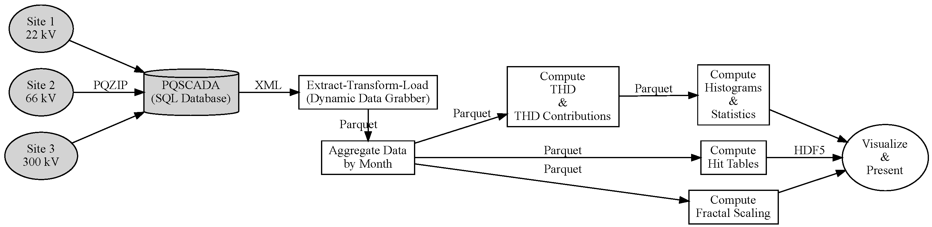
2.1. Data Origin

SINTEF has conditional access to power quality data for the majority of the Norwegian power system through agreements with distribution system operators (DSOs) and the Norwegian transmission system operator (TSO) Statnett. The data cover the period from January 2009 to early March 2020. The nominal line voltages at the locations where the measuring instruments are installed varies from 10 to 420 kV. A total of roughly 270 years of PQ data have been collected from 49 measurement nodes, giving on average 5–6 years of historical data from each node. However, the number of years of available data varied significantly from node to node.

In this work, we focus on three sites as full coverage of the available data would either: (i) require a different analytical approach; or (ii) clutter the presentation needlessly. The three sites were chosen to have different voltage levels, are placed in different locations in the Norwegian power grid and have long and robust time series. In conjunction, these sites constitute the basis for the below analysis and discussion.

All sites are located in the Norwegian grid so they are exposed to the Norwegian power mix, barring bottlenecks between price zones. The power mix is dominated by power from hydroelectric plants (85%), followed by biomass (12%) and wind (4%) [65], (data from 2018).

2.2. Data Flow, Extraction, and Processing

Raw data are recorded by Elspec Power Quality Analyzers (PQAs), https://www.elspec-ltd.com/metering-protection/ (accessed on 26 April 2022) compressed, and then forwarded to a PQSCADA, https://www.elspec-ltd.com/power-quality-software-pqscada-software/ (accessed on 26 April 2022) database for permanent storage. The Elspec PQAs sample voltage, current, power waveforms at up to $50\mathrm{kHz}$, but employ lossy compression (at the edge) to reduce the data volume and velocity. Due to their proprietary nature, the details of the compression are not well documented. The PQSCADA database can be queried for a wide range of performance parameters, including—but not limited to—aggregated voltage and harmonics data. We extract data from this database through a small stack of Python [66] scripts that abstract away various data engineering complications. These depend heavily on Numpy [67] and Pandas [68].

We extract data from sites at three different grid voltage levels. For each level, there are two data packages. The first covers four years, six voltage (three phase-to-ground, three phase-to-phase) channels, and eight harmonics. The second covers a month, three voltage channels (phase-to-ground), and 96 harmonics. Data are aggregated by calculating mean values in intervals of $1/50\mathrm{Hz}$. Each site in the first (second) package contains $3.6\times {10}^{11}$ ($3.9\times {10}^{10}$) samples. See also

Table 1. We extract two data packages. The first covers four years, six voltage channels, eight harmonics. The second covers a month, three voltage channels, 96 harmonics. They contain $3.6\times {10}^{11}$ and $3.9\times {10}^{10}$ samples, respectively.

Site	Voltage	Period	${\mathit{V}}_{\mathbf{Phases}}^{\mathbf{Harmonics}}$	Aggregation
1	$22\mathrm{kV}$	2015 to 2018	$V_{1,2,3,12,23,31}^{0\cdots 8}$	$1/50\mathrm{Hz}$, Mean
2	$66\mathrm{kV}$	2015 to 2018	$V_{1,2,3,12,23,31}^{0\cdots 8}$	$1/50\mathrm{Hz}$, Mean
3	$300\mathrm{kV}$	2015 to 2018	$V_{1,2,3,12,23,31}^{0\cdots 8}$	$1/50\mathrm{Hz}$, Mean
1	$22\mathrm{kV}$	January 2017	$V_{1,2,3}^{0\cdots 96}$	$1/50\mathrm{Hz}$, Mean
2	$66\mathrm{kV}$	January 2017	$V_{1,2,3}^{0\cdots 96}$	$1/50\mathrm{Hz}$, Mean
3	$300\mathrm{kV}$	January 2017	$V_{1,2,3}^{0\cdots 96}$	$1/50\mathrm{Hz}$, Mean

.

Uncompressed sizes for the data packages are $\sim 2.8\mathrm{TB}$ and $240\mathrm{GB}$, respectively. To deal with this amount of data efficiently, we use column storage with lossless compression (Parquet (https://parquet.apache.org (accessed on 26 April 2022))) and slice data into subsets for processing.

2.3. Data Processing: THD and Harmonic Contributions

For each harmonic component, querying the database of Elspec data returns the harmonic voltage as a fraction of the fundamental voltage component. We use this value (i) directly, (ii) to calculate THD, and (iii) to calculate the contribution of the harmonic to THD. This is done as follows.

For the i-th phase, the voltage in the j-th harmonic is $v_{i,j}=c_{i,j}{v}_{i,0}$, where $c_{i,0}$ is the value returned by the device. $v_{i,0}$ is the value of the fundamental voltage of the i-th phase. The THD for the i-th phase is:

$${\mathrm{THD}}_i=\frac{\sqrt{{\sum }_{j=1}^{j,\max }{v}_{i,j}^2}}{\sqrt{v_{1,0}^2}}=\sqrt{{\displaystyle {\sum }_{j=1}^{j,\max }}{c}_{i,j}^2},$$

and the contribution of the j-th harmonic to the overall THD is $c_{i,j}^2/{\mathrm{THD}}_i^2$. Depending on the site and temporal coverage, data is available for either 8 or 96 harmonics ($j,\max =\{8,96\}$ as well as phase-to-ground ($i=\{1,2,3\}$) or phase-to-phase voltages ($i=\{12,23,31\}$).

2.4. Data Processing: Cumulative Distribution Functions, Histograms, and Percentiles

Statistical analysis of data in this work is fairly standard although some adaptions are made to deal with the large volumes. We explore and present the statistical distributions of measurements using their (normalized) cumulative distribution distribution functions (CDFs). For some variable x (for example, THD measurements), the normalized CDF is $\mathcal{C}\left(x\right)={\int }_0^x\rho \left(x^{\prime }\right)\mathrm{d}{x}^{\prime }/{\int }_0^{\infty }\rho \left(x^{\prime }\right)\mathrm{d}{x}^{\prime }$, where $\rho \left(x\right)$ is the probability density function of x. For a finite number of samples, $\mathcal{C}$ and $\rho$ can be approximated by computing the (cumulative) histogram of x. In other words, given N samples, $\mathcal{C}\left(x_t\right)=N(x<x_t)/N$ is the fraction of samples with values of x below some threshold $x_t$.

Owing to the large amounts of data, we calculate histograms individually for each voltage channel and harmonic order in time-slices of one month. The histograms over the entire time-period are then the sums of the monthly histograms. The cumulative histograms are then computed as their cumulative sum.

All percentiles in our analysis are approximate. The standard (exact) way of calculating percentiles requires loading (and sorting) all samples in memory, which proved difficult. Instead, we estimate percentiles from the cumulative distribution functions. Numerically, for the desired percentile $\mathcal{P}$, this amounts to finding the value of $x_t$ at $\mathcal{P}=\mathcal{C}$. This means that the numerical accuracy of our percentile calculations is limited by the binning used during histogram calculation. We use 256 logarithmically spaced bins in the range $0.01$ to 10, corresponding to an upper bound on the numerical accuracy of $\approx {10}^{-2}$.

2.5. Data Processing: Time-Distribution of THD Excursions

While our dataset has no information about whether events (e.g., voltage drops, rapid voltage changes, interruptions, or earth faults) occur, we can nevertheless try to understand how the largest excursions (outliers) of harmonic power behaves. In other words, we wish to determine how the largest values of harmonic power are distributed in time. Do they occur regularly? Do they cluster together? Does their distribution depend on the time-scale?

We characterize the time-distribution of excursions by determining the fractal dimension $\mathcal{D}$ of a downsampled and binarized THD signal. For each minute, we determine whether any of the samples therein have a value exceeding the 99 percentile of the (four-year) THD distribution. If it does, the minute is tagged as containing an outlier (and vice versa). We then calculate $\mathcal{D}$ by box-counting (and slope-fitting) the binarized time-series [69]. This method essentially asks how many boxes $N\left(s\right)$ of a given size s (the time-scale) are required to completely cover the binary signal. The fractal dimension is the slope $\mathcal{D}$ of the power-law $N{s}^{-\mathcal{D}}$. We compute $\mathcal{D}$ from least-squares regression of ${log}_{10}\left(N\left({log}_{10}s\right)\right)$. For a given time-scale s, $\mathcal{D}=1$ indicates that excursions are uniformly distributed. Conversely, $\mathcal{D}<1$ indicates temporal clustering of excursions. We consider a range $s_{\min }\le s\le s_{\max }$ with $s_{\min }=300\mathrm{s}$ (five times the time-resolution of our binary signal) and $s_{\max }=292\mathrm{days}$ (a fifth of the four year measurement period).

2.6. Challenges

During data extraction and initial data exploration, we have encountered three challenges that constrain our analysis.

• Compression Thresholds—The ELSPEC PQA instruments have a compression algorithm that introduces a lower cut-off level for the harmonic components in their compression algorithm. Contributions to the overall signal below this cut-off value for each harmonic component will not be recorded in the stored data from the instrument. This threshold may vary between measuring devices, depending on the harmonic noise and the needs of the measurements at the given site. The threshold is usually set to be in a range from $0.1$ to $0.2$% of the base harmonic component. Values below this level will be stored as 0 values, and is referred to as such in the discussion below.
• Computational Tractability—We had initially set out to load 96 harmonics and six voltages for all three nodes over the four year time period. However, the database proved uncooperative and required frequent restarts during the extraction. We therefore limited the analysis of 96 harmonics to a month.
• THD Calculation—The Elspec instruments also record THD directly, although neither the aggregation interval nor function is clearly documented. We observe a median difference of 21% (ranging from 0 to 56% at the 1 and 99 percentile, respectively) between the THD calculated by our own procedure and the THD directly reported by the Elspec instrument. We base the analysis in this paper on the above THD calculation for transparency reasons.

3. Results

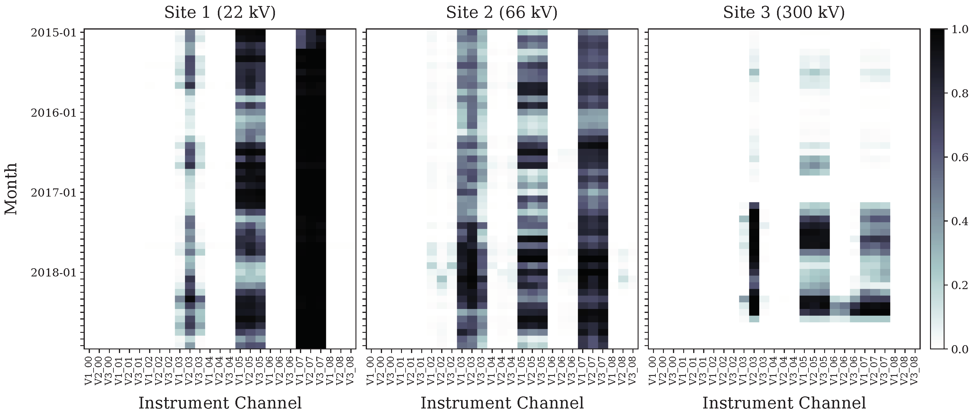
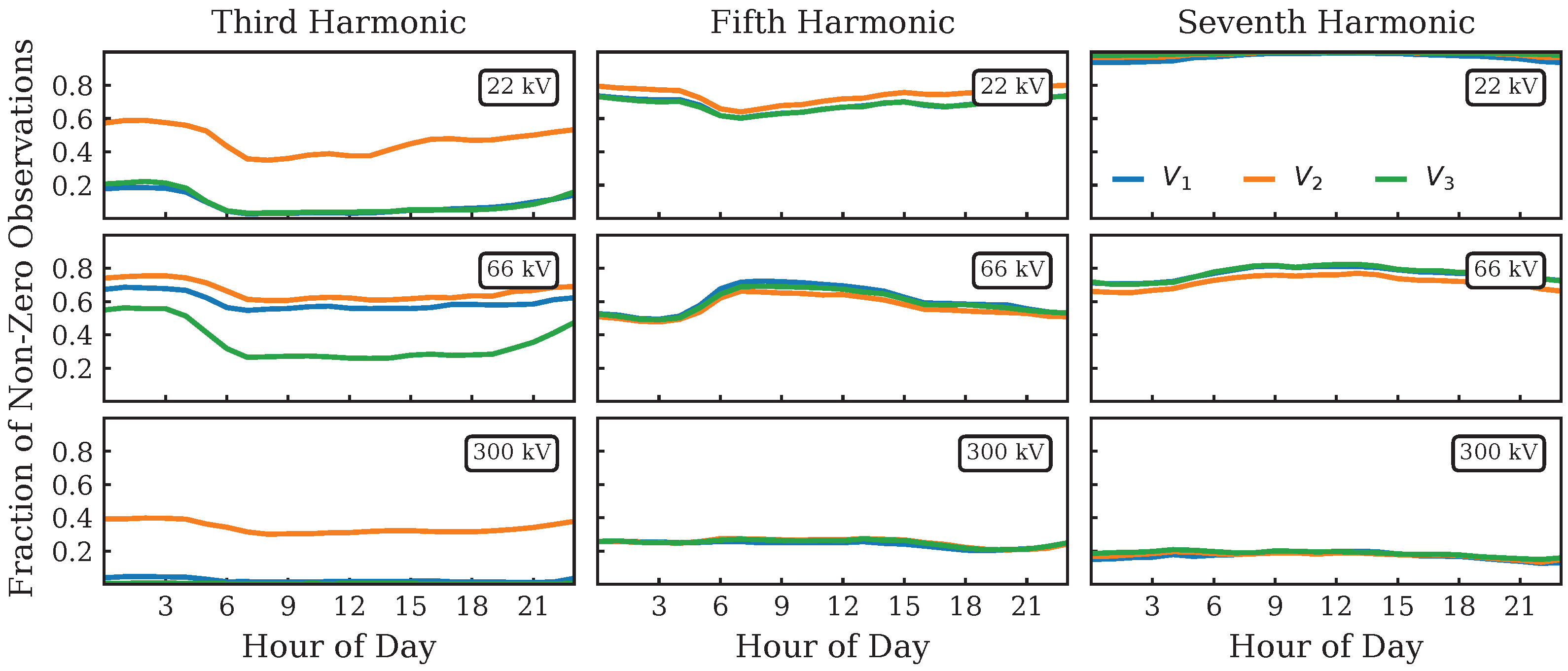
3.1. Presence of Harmonics

Figure 3 shows the fraction of cycles (per month) with power $>0$ for three sites in the Norwegian power grid between 2015 to 2018. By grouping data by harmonic channel, phase, month, and site, we find the following.

• Across all voltage levels, non-negligible amounts of non-zero measurements occur only on the third, fifth, and seventh harmonics;
• At the $22\mathrm{kV}$ level and across all phases, 95% of measurements of the seventh harmonic are non-zero. For the fifth harmonic, there are non-zero measurements in 70% of cases. The third harmonic differs across phases. On $V_2$, non-zero measurements are more common (40%) than on $V_1$ and $V_3$ (10% each). Non-zero observations on the third and fifth harmonic are clustered in time rather than being spread out evenly. The clusters are not evenly distributed and do not appear to correlate with seasons;
• At the $66\mathrm{kV}$ level, we find the same patterns as at the $22\mathrm{kV}$ level, with most non-zero measurements found in the seventh, fifth, and third harmonics. Across all phases, we find non-zero values for the seventh and fifth harmonics in 75 and 55% of cases, respectively. For the third harmonic, non-zero values are unbalanced across phases. On $V_1$, $V_2$, and $V_3$, we count 55, 65, and 35% of non-zero values, respectively. Observing no differences in the temporal distribution of counts, $V_3$ appears to have a generally lower level of non-zero counts;
• At the $300\mathrm{kV}$ level, there is a marked difference between the periods of March 2017 to July 2018 and the remainder of the observation period. Inside this period, 45% of measurements across phases (and for the third, fifth, and seventh harmonic channel) are non-zero. Outside this period (and overall), only 3 (19)% of measurements are non-zero (again, for the third, fifth, and seventh harmonic channel). The temporal patterns (in the period of March 2017 to July 2018) are identical across phases, except for the third harmonic channel on $V_2$, where 87% of all samples are non-zero (compared to 45 and 55% for the third and fifth harmonic, respectively).

The harmonic levels in Figure 4 and Figure 5 show that there is some variation in harmonic levels on each site. The figures show variation detailed by harmonic number, voltage level and hour-of-day (Figure 4) and the cumulative distribution function (CDF) for each voltage level (Figure 5). As mentioned above, the non-zero values on Site 1 ($22\mathrm{kV}$) are present on the 3, 5 and 7 harmonics. The presence of these odd harmonics is usual in the modern power system, due to a high number of non-linear loads [70]. Both single- and three-phase converters are contributing to this type of harmonic noise, for equipment such as computers and power-intensive industry, respectively. For Site 1, the 7 harmonic is higher than 1% for the whole analysed period. The 5 harmonic also has a considerable presence throughout the period. This could suggest that the harmonic noise is caused by power-intensive industry with 6-pulse three-phase rectifiers [71]. Based on the results in Figure 4, it is clear that there is a daily variation in the harmonic levels that backs this claim.

Figure 3. Fraction of non-zero observations for the first eight harmonics in each voltage channel (denoted as Instrument Channel), grouped by harmonic. Data for all three sites are shown, see panel titles. A period of four years is covered for each site. The fraction (see colormap on the right) is calculated over $\sim 1.3\times {10}^8$ samples in each month. It is clear that there are some channels (harmonics for each phase) that are clearly more present than others, and that the pattern is to a large degree transferable from phase to phase and from site to site. It is also clear that there is considerably less harmonic content in the higher voltage levels. This is confirmed in Figure 5 and Figure 6.

Figure 3. Fraction of non-zero observations for the first eight harmonics in each voltage channel (denoted as Instrument Channel), grouped by harmonic. Data for all three sites are shown, see panel titles. A period of four years is covered for each site. The fraction (see colormap on the right) is calculated over $\sim 1.3\times {10}^8$ samples in each month. It is clear that there are some channels (harmonics for each phase) that are clearly more present than others, and that the pattern is to a large degree transferable from phase to phase and from site to site. It is also clear that there is considerably less harmonic content in the higher voltage levels. This is confirmed in Figure 5 and Figure 6.

Figure 4. Variation in the occurrence of non-zero values for each node averaged on a daily basis. The 3, 5 and 7 harmonics have been selected.

Figure 4. Variation in the occurrence of non-zero values for each node averaged on a daily basis. The 3, 5 and 7 harmonics have been selected.

Figure 5. Cumulative distribution function (CDF) of total harmonic distortion (THD) for three sites (columns). We use 256 bins of uniform logarithmic spacing from ${10}^{-2}$ to 10. Distributions are calculated over the time range from 2015 to 2018 for a total of $\sim 5.9\times {10}^9$ samples. Top: CDFs for each phase (see legend). Bottom: Difference between the CDFs for $V_2$ and $V_1$ as well as $V_3$ and $V_1$, respectively (see legend). Statistically, the three phases always remain within six percent of each other. See

Table 2. Summary statistics for the distribution of total harmonic distortion (THD) per site and phase.

Site	Phase	1 Percentile	Median	99 Percentile
$22\mathrm{kV}$	$V_1$	$0.15$	$0.49$	$1.48$
	$V_2$	$0.19$	$0.51$	$1.48$
	$V_3$	$0.19$	$0.51$	$1.48$
$66\mathrm{kV}$	$V_1$	$0.04$	$0.29$	$1.01$
	$V_2$	$0.05$	$0.31$	$1.13$
	$V_3$	$0.05$	$0.32$	$1.26$
$300\mathrm{kV}$	$V_1$	$0.05$	$0.24$	$0.73$
	$V_2$	$0.05$	$0.28$	$0.73$
	$V_3$	$0.05$	$0.25$	$0.77$

for summary statistics.

Figure 5. Cumulative distribution function (CDF) of total harmonic distortion (THD) for three sites (columns). We use 256 bins of uniform logarithmic spacing from ${10}^{-2}$ to 10. Distributions are calculated over the time range from 2015 to 2018 for a total of $\sim 5.9\times {10}^9$ samples. Top: CDFs for each phase (see legend). Bottom: Difference between the CDFs for $V_2$ and $V_1$ as well as $V_3$ and $V_1$, respectively (see legend). Statistically, the three phases always remain within six percent of each other. See Table 2 for summary statistics.

Figure 6. Cumulative distribution function (CDF) of total harmonic distortion (THD) for three sites (see legend) for the phase-to-ground voltage $V_1$ plotted together for comparison. Binning and data basis is the same as for Figure 5. (Top): CDFs for each site (see legend). (Bottom): Difference between the CDFs for 22 and $300\mathrm{kV}$ as well as the 66 and $300\mathrm{kV}$ sites, respectively (see legend). See Table 2 for summary statistics. For higher voltage levels, the distribution shifts to smaller THD values—there is less noise in the system.

Figure 6. Cumulative distribution function (CDF) of total harmonic distortion (THD) for three sites (see legend) for the phase-to-ground voltage $V_1$ plotted together for comparison. Binning and data basis is the same as for Figure 5. (Top): CDFs for each site (see legend). (Bottom): Difference between the CDFs for 22 and $300\mathrm{kV}$ as well as the 66 and $300\mathrm{kV}$ sites, respectively (see legend). See Table 2 for summary statistics. For higher voltage levels, the distribution shifts to smaller THD values—there is less noise in the system.

On Site 2 ($66\mathrm{kV}$), there is a similar harmonic pattern as on Site 1, with the most dominant harmonics being the 3rd, 5th and 7th. However, on this site, the 3rd is more dominant. This is a normal observation on this power level. In addition to these odd harmonics, there is a presence of even harmonics on the 2nd, 4th and 8th harmonics. The presence of even harmonics is more important to monitor, as they can cause early degradation and malfunction in the power system [72]. In the analysed period, however, the harmonic level never exceeds 8%, which is the acceptable 10-min average according to the Norwegian regulators requirements [73].

On Site 3 ($300\mathrm{kV}$), there is a similar harmonic pattern as on Sites 1 and 2, except that the harmonic levels are lower than on the other sites throughout the period. There are also some considerable even harmonic levels present on the 6th harmonic. It is also interesting to observe that the harmonic levels are considerably higher during the period from March 2017 to July 2018. The reason for this is not clear to the authors, but it could be caused by a change of topology due to maintenance or construction of a new line in the area during this period. It is also likely that the other seasonal variations that are present during the period from 2015–2018 are caused by changes in topology, including the changes in power generation in the area. The power generation in the areas around the analysed sites is dominated by hydro-power (and to some extent wind-power) plants, and changes in grid-connected generating units can affect the short-circuit impedance of the grid and the associated propagation of harmonic distortion [74]. For grid-connection points with a voltage level from $35\mathrm{kV}$ to $245\mathrm{kV}$, the 10 min average of the 6th harmonic should be below 0.5% [73].

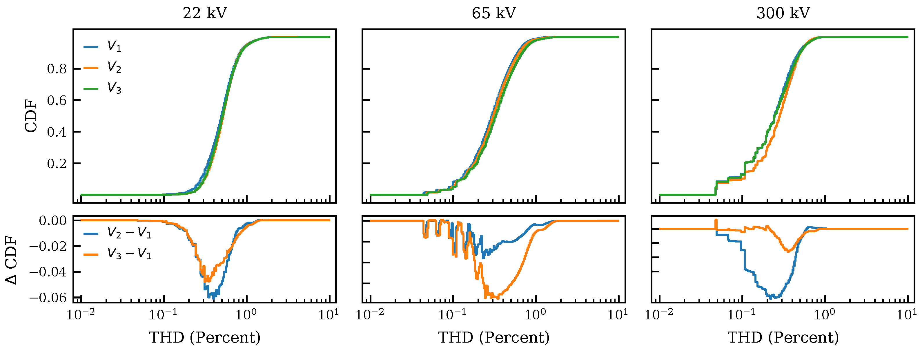
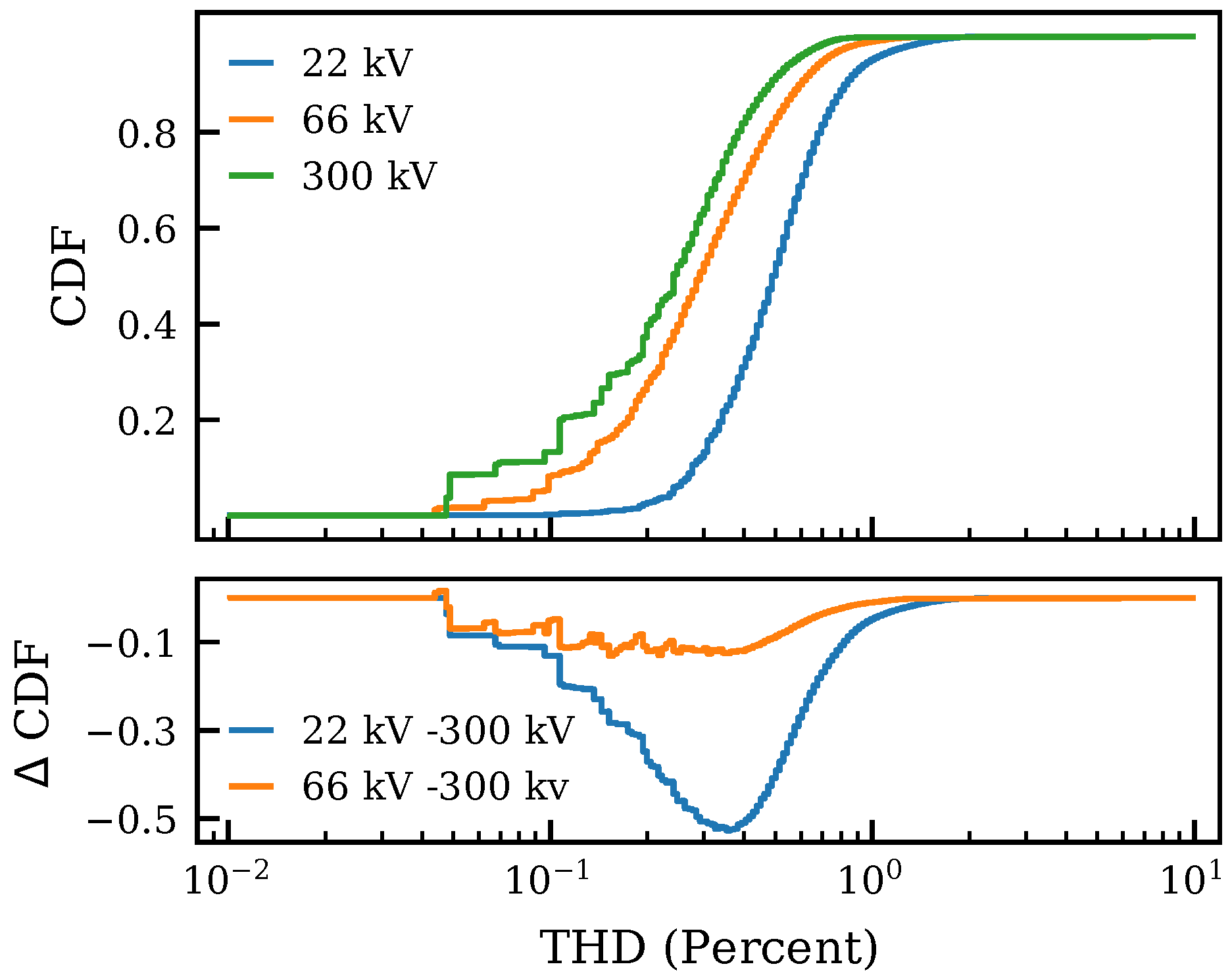
3.2. Total Harmonic Distortion, Phases & Voltage Levels

Figure 5 and Figure 6 show the normalized cumulative distribution functions (CDF) of total harmonic distortion (THD), i.e., the fraction of samples $N(\ge \mathrm{THD})/N$ found at or above a given THD level. Table 2 shows their respective summary statistics. We observe the following:

• Overall, most ($99\%$) of the THD values are small and $\lesssim 1\%$ of their respective fundamental phase voltage. Distributions are narrow with most values concentrated in the range $0.1$ to 1%. Difference between different phases at the same voltage level are always smaller than differences between voltage levels;
• Across phases and voltage levels, the difference between phases is always $\le 6\%$. Note that this only means that the phases are STATISTICALLY within $6\%$ of one another. At any given point in time, their difference may be larger than that;
• Difference between phases cover a wider range of THD for higher voltage levels. The largest integral difference (The area between ${\mathrm{CDF}}_i$ and ${\mathrm{CDF}}_j$, i.e., $\int \sqrt{{({\mathrm{CDF}}_i-{\mathrm{CDF}}_j)}^2}\mathrm{d}\mathrm{THD}$.) between two phases is $0.024$, $0.49$, and $0.056$) for 22, 66, and $300\mathrm{kV}$, respectively. For $22\mathrm{kV}$, the median values of $V_1$, $V_2$, and $V_3$ remain within 4% of one another. This difference grows to 10% and 15% at 66 and $300\mathrm{kV}$, respectively;
• At higher voltage levels, the distributions of THD consistently shift towards smaller values. For $22\mathrm{kV}$ (66, 300), $99\%$ of THD measurements (on $V_1$) are ≤1.48 (≤1.01, ≤0.73). Median THD values shift similarly so that the median THD (on $V_1$) at $300\mathrm{kV}$ ($66\mathrm{kV}$) is half (a fifth) of that measured at $22\mathrm{kV}$. The $22\mathrm{kV}$ site is consistently about half a decade above the $300\mathrm{kV}$ site, and the $66\mathrm{kV}$ site is located between these a little towards the $300\mathrm{kV}$ site.

Regulatory requirements for THD levels are stricter for higher voltage levels, and more effort is made to keep these disturbances low at transmission level due to the potential impact on all downstream distribution feeders. The THD values are usually higher at lower voltage levels due to the proximity to the non-linear harmonic generating loads and generators. The propagation of harmonics from the polluter to higher voltage levels will usually be damped either by damping in grid components (lines, transformers etc.). However, in some cases, active or passive filters may be necessary to make sure that the harmonics do not propagate and cause damage to grid customers elsewhere in the grid. It is, however, important to understand the frequency-dependent impedance of the grid to understand the harmonic propagation and accurately calculate the resonance frequency [72]. As an example, a temporary change of topology in an area of the power system could cause harmonic levels to increase with several orders of magnitude, which as a consequence could cause instability in the power system. In general, the higher the frequency, the higher the resistance is. Consequently, damping of harmonics is stronger at higher frequencies.

Researchers or technicians that seek to utilize the development of THD level or the level of specific harmonics for predictive modelling need to take this variation in harmonic levels into account while designing and training models. This variation in harmonic levels may be an underlying reason why general-purpose models trained on data from many sites in different geographic locations may have an inferior performance compared to models trained on specific sites, even though the data volumes are considerably smaller [75].

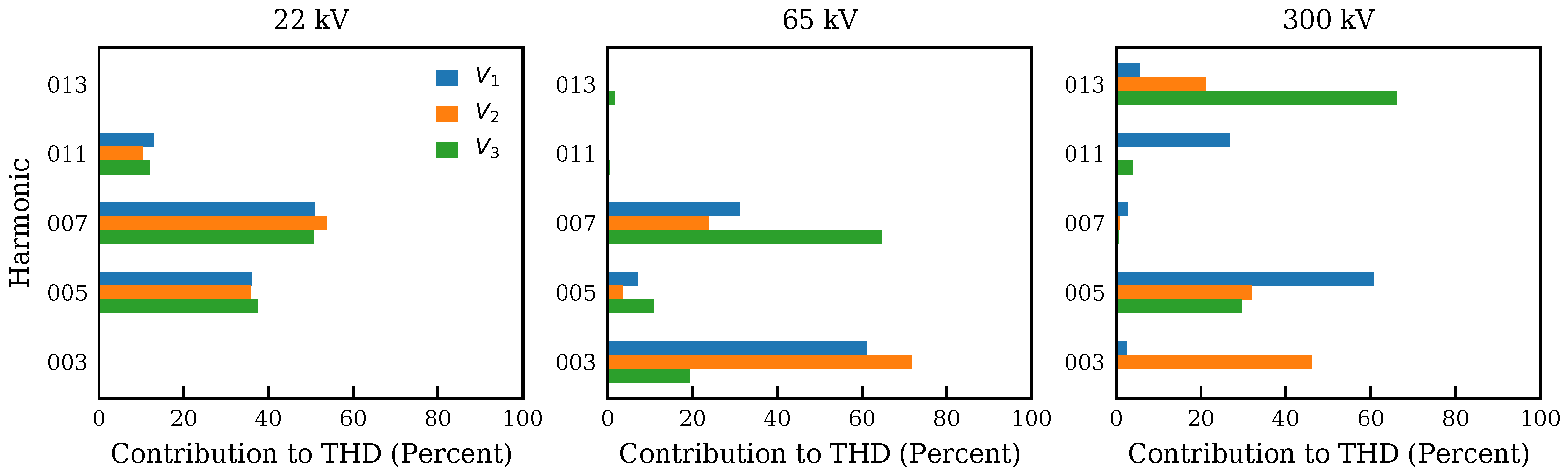
3.3. Harmonic Contributions to Total Harmonic Distortion

In the previous subsection, a high-level picture of harmonic noise in the power system was established through an analysis of the THD level on the three investigated sites. In this subsection, the contribution from each of the individual harmonics on the THD is investigated. This will allow us to answer: (i) how many harmonics contribute (meaningfully) to the THD on different voltage levels; (ii) to what extent they are contributing; and (iii) whether there are differences in the most relevant harmonics across voltage levels. As indicated in Section 2, we consider only the month of January 2017 due to the large volume of data. Although only harmonics up to the 7th order is shown in the figures, harmonics up to the 96th order has been extracted and used for analysis. Figure 7 illustrates the average contribution of each individual harmonic to the THD over a time period of one month. The following can be concluded.

• Across all phases and voltage levels, ≳98% of the contribution towards the THD are concentrated in at most the 13th harmonic. The next largest contributions ($1.9$ percent) is the 29th harmonic on $V_3$ in the $66\mathrm{kV}$ site. Beyond this, all other contributions are ≲1%;
• The highest individual harmonic with a total contribution of ≳2 % are 11th ($22\mathrm{kV}$), 13th ($66\mathrm{kV}$), and 13th ($300\mathrm{kV}$). At 22 and $300\mathrm{kV}$, these harmonics also have a significant (>10%) contribution on at least one phase. However, at $66\mathrm{kV}$, the largest harmonic with a significant contribution is the 7th;
• At $22\mathrm{kV}$, the 7th, 11th, and 5th harmonic contribute the most to THD. In order (and averaged over phases), they contribute ∼52, 37, and $11\%$. Across phases, the contributions to THD are balanced and remain within a few % of one another;
• At $66\mathrm{kV}$, the 3rd, 7th, and 5th harmonics contribute the most to the THD. When averaged over all phases, they contribute ∼51, 40, and 7%, respectively. There is an imbalance in the contribution of $V_3$ which contributes 40% more than $V_1$ and $V_2$ to the THD on the 7th harmonic. For the 3rd harmonic, the reverse holds;
• At $300\mathrm{kV}$, there are large differences (20 to 40%) between the contribution of each phase to the THD across different harmonics. For example, on $V_1$, the 5th harmonic dominates THD with a contribution 60%. On $V_3$, however, the 13th harmonic dominates with a 60% contribution. On $V_3$, the 3 harmonic drives THD (with a contribution of ∼50%). The authors are not able to attribute this imbalance to any specific phenomena, and this may be the subject of future investigations.

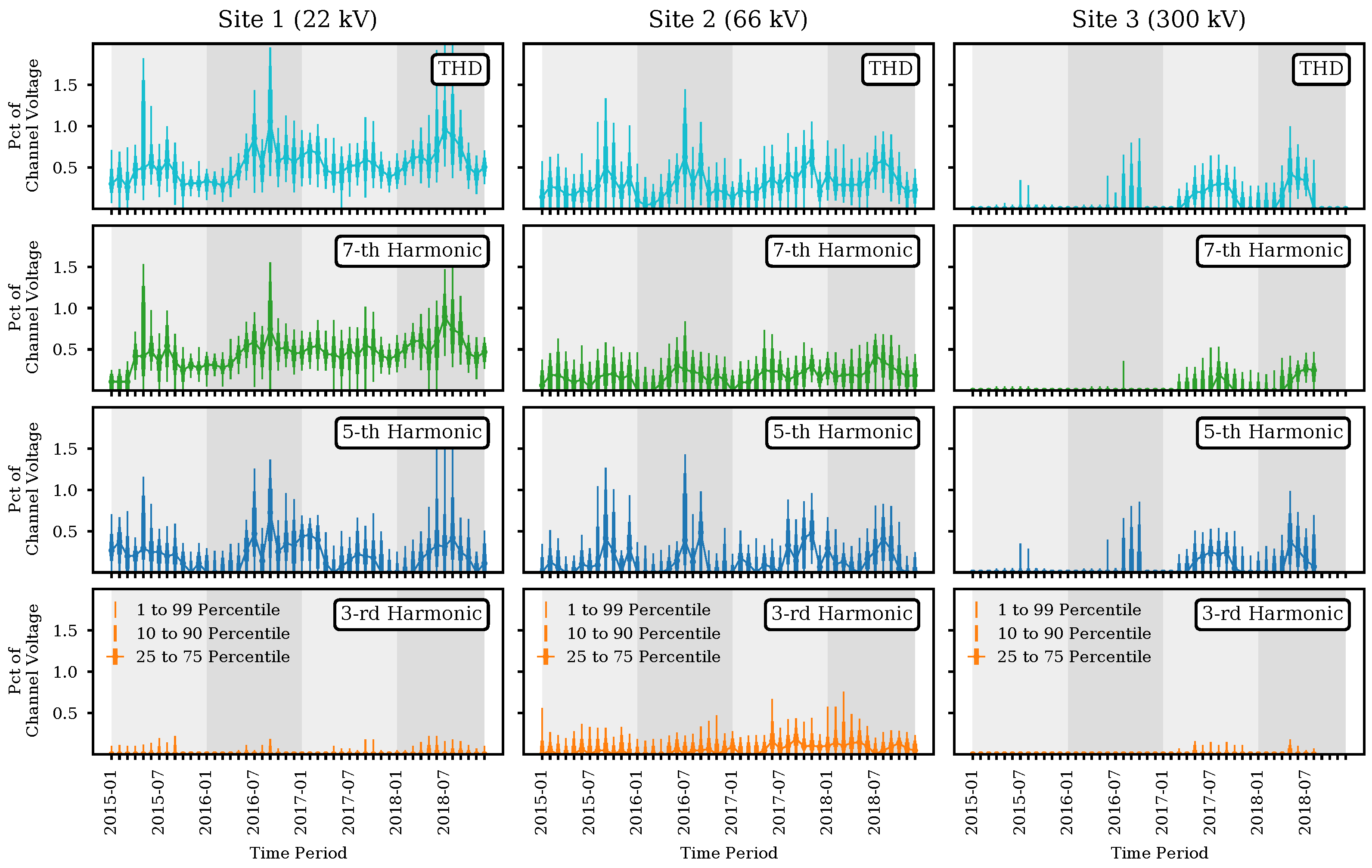
3.4. Harmonic Distortions over Time

After considering the THD and the contributions of individual harmonics, we now extend the analysis to include variations in time. Figure 8 shows the monthly statistics (median, 1 to 99, 10 to 90, and 25 to 75 percentile ranges) for the THD as well as third, fifth, and seventh harmonic for a single phase on all three sites. We find the following.

• For Sites 1 and 2, non-zero THD values are present during the entire measurement period from 2015 to 2018. For site 3, only 16 out 24 months in 2015 and 2016 and 18 out of 24 months between 2017 and 2018 record THD values above the compression threshold;
• For all sites, THD appears to follow a seasonal pattern. For Site 1 and Site 2, median THD is about 50% higher in summer and autumn than during the winter and spring. For Site 3, the difference is more pronounced due to many periods without observed THD. For 2015 and 2016, non-zero THD values are recorded only in the summer months;
• The spread (difference between the 1 and 99 percentile) of observed THD values (binned monthly) decreases with voltage level. Aggregating across months, the maximum spreads are $1.71$, $1.45$, and $1.00$% for Sites 1, 2, and 3, respectively. In the same order, the average spreads are $0.73$, $0.67$, and $0.27$%. Independent of voltage level, larger spreads always occur in the summer and autumns months;
• For Site 1 (and phase 1), the contribution of the third, fifth, and seventh harmonics to THD over a period of 48 months is in-line with the results for a single month (cf. Figure 7). Over time, the majority of THD is accounted for by the 5th and 7th harmonics. For most months, both harmonics track similar medians (and spreads), except in the spring and autumn of 2017. Over these periods, the 5th harmonic follows a seasonal pattern (lower during winter/spring, larger during summer/autumn) while the 7th harmonic keeps an almost constant median. Their combined contribution leads to the deviation from seasonality earlier observed in THD;
• For Sites 2 and 3, the contribution of individual harmonics to THD is more complicated. For Site 2, considering only January 2017 suggests that the 3rd and 7th harmonic should contribute most to THD. However, over time, we observe a different pattern. Here, the 7th harmonic appears to set a baseline of distortion (with slight seasonality), the 5th harmonic modulates additional (stronger) seasonality in the median as well as additional noise (larger spread), and the 3rd harmonic adds even more noise (larger spread). This shows that the analysis of a single month is insufficient and unlikely to be representative of THD and harmonic contributions over longer time frames.

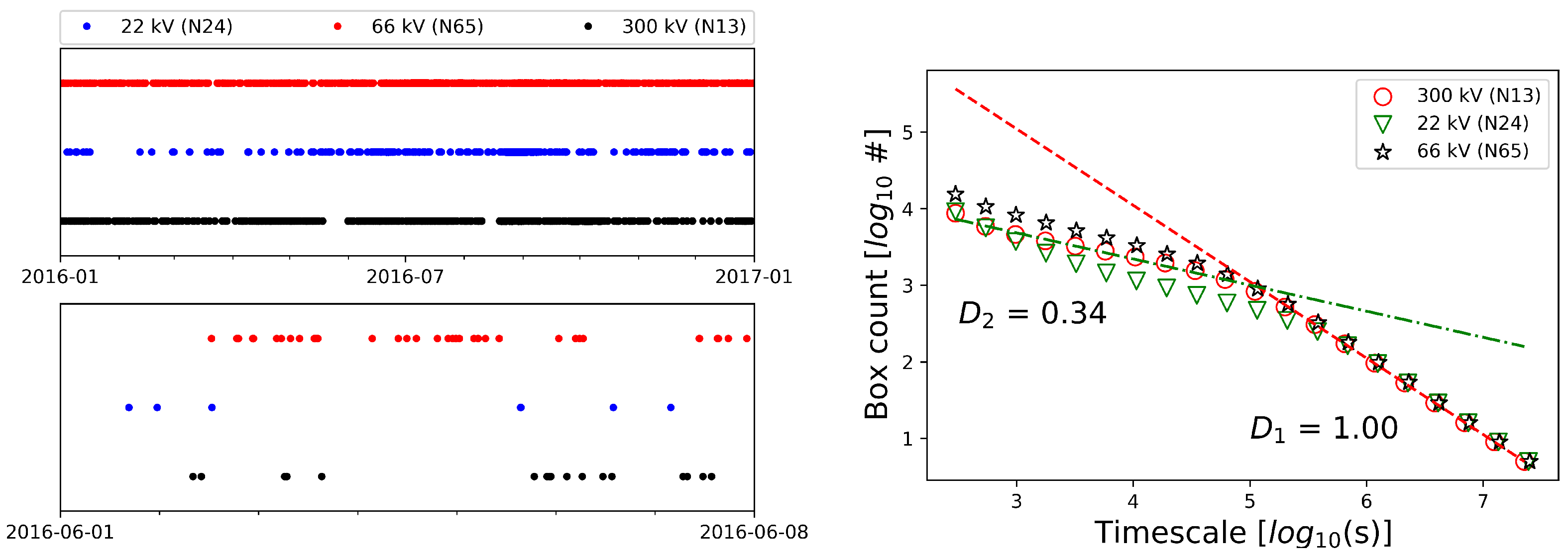
3.5. Temporal Distribution of THD Excursions

Previous work [60] suggests that events in the power grid are not uniformly distributed in time, but rather occur in clusters. While not having access to event data, we can analyze the temporal distribution of THD excursions (values $>99$ percentile) for the three sites on a signal downsampled a time-resolution of one minute. For each site, there are a total $\sim 2\times {10}^6$ samples (minutes). For the 22, 66, and $300\mathrm{kV}$ sites, we find 34362, 39015, and 22063 min with excursions, respectively.

Figure 9 show a temporal scatterplot of THD excursions as well as the fractal dimension $\mathcal{D}$ as a function of time-scale s, on the left and right panel respectively. We find that—irrespective of voltage level—the fractal dimension $\mathcal{D}$ depends on the time-scale. In particular:

• At timescales $300\mathrm{s}<s\le {10}^5\mathrm{s}$ (a few days), we find $\mathcal{D}\sim 0.34<1$ (with slight variations across voltage levels, but a goodness of fit $R\sim 0.99$ for each level). This suggest multi-scale substructure of THD excursions in time. Visually, this is manifested as clumping of THD excursions (see Figure 9, lower panel). Clusters also vary in size (duration) and can be decomposed into further (sub-)clusters;
• At time-scale $s\ge {10}^5\mathrm{s}$, we find $\mathcal{D}\sim 1$ ($R\sim 0.99$). This suggests no (or at least very little) temporal substructure in the distribution of THD excursions. Visually speaking, there are long sequences of THD excursions with similar timing (Figure 9, upper panel). There are only occasional large gaps in time.

The fractal dimension is essentially a measure of signal roughness. At timescales $\gtrsim {10}^5\mathrm{s}$, our binary signal of THD excursions is fairly smooth (visually, excursion appear equally spaced in time). Statistical measures will weakly depend on the timescale over which they are calculated. For example, the mean return interval computed over a period of a weeks, a months, or years will be similar. At timescales $\lesssim {10}^5\mathrm{s}$, excursions clump together (the signal is rough) so that statistical measures will strongly depend on the timescale over which they are calculated. The mean return intervals computed over a few minutes or over a few hours will be different.

Published works using fractal analysis apply a variety of measures and is therefore difficult to compare to. For example, refs. [76,77] compute the fractal dimensions of one-dimensional time-series (of power and current, respectively) to detect the presence of (artificially induced) events and loads. Closest to our work is [78], which computes the Hurst exponent $\mathcal{H}$ of a (presumably binarized) power fault time-series to determine the timescales over which faults in transmission (and distribution systems) are correlated.

While $\mathcal{D}$ measures local roughness, $\mathcal{H}$ measures long-term correlations. (Values $\mathcal{H}>0.5$ indicate long-term dependencies, while $\mathcal{H}<0.5$ indicates rapid mean reversion.) For self-similar (self-affine) processes, $\mathcal{D}=n+1-\mathcal{H}$ ($n=0$ for a binarized time-series), so that locally defined roughness can be related to long-term correlations [79]. For $\mathcal{D}=0.34$ and $\mathcal{D}=1$, we find $\mathcal{H}=0.66$ and $\mathcal{H}=0$, respectively. In our case, this means that long-term correlations are limited to timescales $\lesssim {10}^5$ s. In other words, the autocorrelation drops off at lags $\gtrsim {10}^5\mathrm{s}$ and phenomena longer than a few days ago do not influence THD excursions. By directly computing $\mathcal{H}$, ref. [78] find $\mathcal{H}\sim 0.74$ ($0.78$) for transmission (distribution) system faults over a time period of a few hundred days, indicating that the power system faults have much longer correlation timescales than THD excursions. (We have not tested for self-similarity so that any comparison that involves computing $\mathcal{H}$ from $\mathcal{D}$ (instead of directly from the signal) should be taken with a grain of salt.)

4. Discussion

In this section, we summarise the discussion of the implications from the findings observed in the results section above and try to indicate the consequences for the application of data-driven predictive modelling.

4.1. Regulation on Harmonic Distortion

In Section 3.2, we found that THD and harmonic power remains well below the Norwegian regulatory requirements of $\le 8$% of the RMS voltage on the phase [73]. However, there is considerable variation across nodes, timescales, and seasons. Methodologies utilizing harmonics observations must therefore account for these. Variations can be accounted for implicitly (left to be dealt with by the model) or explicitly (by encoding into auxiliary features). Implicit processing requires sufficiently complex models (e.g., deep neural networks) while explicit encoding requires engineering of suitable features (e.g., information on time and season, node location, as well as other pertinent node metadata).

4.2. Trends in THD and Harmonic Contributions

In Section 3.2, we found that higher voltage levels have lower THD than lower voltage levels (Figure 6), but that there is large variation across phases (Figure 5). Additionally, in Section 3.3, we noted that harmonic channels contribute differently to THD depending on the node (voltage level) and phase. This strongly suggests that there are site specific variations that predictive models can exploit. Explicitly exploiting these variations will require models to be exposed to harmonic information for each phase. As we find very little THD contribution beyond the 13 harmonic (independent of phase and voltage level), models are unlikely to benefit from the inclusion of data for higher orders. This is in line with previous work [80,81].

4.3. Towards Event Prediction

Training and verification of data-driven methods requires a large amount of data to be efficient. In general, more input data will provide a larger learning basis and better results. However, any and all additional data should contain new (uncorrelated) information (rather than redundant information or, even worse, noise). Which data (features) to include is often motivated by domain-expertise, and feature engineering techniques (where features are combined or augmented) can be very effective. In [82], for example, we have demonstrated a procedure to assess the value of adding additional data (or features).

We have found that THD and individual harmonics (across voltage levels, phases, and seasons) vary considerably. It is therefore unlikely that a generalized model trained on data from all sites and phases will perform particularly well for a single site and phase. The potential application of transfer learning techniques can remedy such issues [83]. Transfer learning applies a two-step training procedure. First, a model is trained on data from all sites and phases. Second, the model is refined by exposing it to data from a single target site (and phase). Such an approach is not undertaken in this paper and is left for further works.

4.4. Statistical Robustness and Time-Correlations

In Section 3.5, we have shown that statistical measures (such as the mean return interval of THD excursions) computed over timescales of a more than a few days tend to be robust. Conversely, measures computed over shorter timescales depend on the timescale over which they are computed. Additionally, THD excursions also become uncorrelated if they are more than a few days apart. Taken together, this suggests that predictive models (a) do not need to take into account data more than a few days in the past, and (b) should include features that explicitly model temporal features such as time since last event.

4.5. Actionable Event Predictions

For predictions to be actionable for power system operators, they must be reliable (few or no false alarms), accurate (predict actual events), and timely (sufficient forecast horizon to take action). Actions would aim to mitigate or even avoid the incipient events.

Assuming the first two are met, forecasts on time horizons of a few minutes could trigger a control room response such as reconfiguring the grid or reducing the load on critical components. Over longer time horizons (hours), it may be possible to do field actions such as removing vegetation or wildlife. In some cases, an early warning could also enable early mobilization of personnel to shorten incident response times.

If systems become sufficiently robust and accurate, actions could be initiated without a human in the loop. In this case (and assuming sufficient control capabilities), very short time horizons (milliseconds) may be possible.

5. Conclusions & Future Work

We have presented a statistical analysis of time-series of harmonic components for three sites in the Norwegian power system. Variations between voltage levels, over different time periods (hourly, monthly, and seasonally), and between individual harmonics were quantified. The findings can be condensed into four major points:

• The distribution of harmonics differs with phases and voltage level (site);
• There is little power (below the Elspec instrument cut-off) beyond the 13 harmonic;
• There is temporal clumping of events;
• There is seasonality on different time-scales.

Each of these has an implication for the development of data-driven (machine learning) models of power system behaviour. In particular:

• Variations in harmonic power with phase and voltage level suggests that two-step training procedures akin to transfer learning may be useful. In such a scheme, one would (i) train a baseline model on data from all nodes and all harmonics, and then (ii) fine-tune the model to with data from specific sites. This will result in a model specific to each site;
• The lack of power beyond the 13th harmonic suggests that including higher-order harmonics will not increase the predictive power of models;
• Clumping suggests that models should include features such as the time-since-last-event to distinguish between grid states (frequent alarms vs. nominal operations);
• Seasonality suggests that models should include features such as the hour of the day or the month of the year.

Strictly speaking, these conclusions are only valid for the set of three sites we have analyzed. However, Norwegian grid operators have deployed PQA instruments at 49 sites (with more being rolled out). Most of these have at least a few years worth of measurements (and some more than a decade). Future work should therefore focus on adapting and scaling the analysis to (a) include more sites, (b) account for grid topology (and switching), as well as (c) explicitly account for local production and consumption profiles. Additionally, the statistical properties of voltages, currents, and power should be included to generalize the work even further. An early draft of this work included a preliminary statistical analysis of cycle-by-cycle RMS voltage, but we were forced to drop it due to resource constraints.

A separate thread of work should focus on applying these lessons to the development of predictive models. The development of predictive (machine learning) models comes with its own set of challenges and choices—the inclusion of which we deemed to have gone beyond the scope of this contribution.

References

- Kumar, G.V.B.; Sarojini, R.K.; Palanisamy, K.; Padmanaban, S.; Holm-Nielsen, J.B. Large Scale Renewable Energy Integration: Issues and Solutions. Energies 2019, 12, 1996. [Google Scholar] [CrossRef] [Green Version]
- Muljadi, E.; McKenna, H. Power quality issues in a hybrid power system. IEEE Trans. Ind. Appl. 2002, 38, 803–809. [Google Scholar] [CrossRef]
- Rönnberg, S.; Bollen, M. Power quality issues in the electric power system of the future. Electr. J. 2016, 29, 49–61. [Google Scholar] [CrossRef]
- Balasubramaniam, P.M.; Prabha, S.U. Power Quality Issues, Solutions and Standards: A Technology Review. J. Appl. Sci. Eng. 2015, 18, 371–380. [Google Scholar] [CrossRef]
- Sallam, A.A.; Malik, O.P. Electric Distribution Systems; Wiley-Blackwell: Hoboken, NJ, USA, 2018; pp. 1–604. [Google Scholar]
- Bashir, A.K.; Khan, S.; Prabadevi, B.; Deepa, N.; Alnumay, W.S.; Gadekallu, T.R.; Maddikunta, P.K.R. Comparative analysis of machine learning algorithms for prediction of smart grid stability. Int. Trans. Electr. Energy Syst. 2021, 31, e12706. [Google Scholar] [CrossRef]
- Azad, S.; Sabrina, F.; Wasimi, S. Transformation of smart grid using machine learning. In Proceedings of the 29th Australasian Universities Power Engineering Conference (AUPEC), Nadi, Fiji, 26–29 November 2019; pp. 1–6. [Google Scholar]
- Rangel-Martinez, D.; Nigam, K.; Ricardez-Sandoval, L.A. Machine learning on sustainable energy: A review and outlook on renewable energy systems, catalysis, smart grid and energy storage. Chem. Eng. Res. Des. 2021, 174, 414–441. [Google Scholar] [CrossRef]
- Hossain, E.; Khan, I.; Un-Noor, F.; Sikander, S.S.; Sunny, M.S.H. Application of Big Data and Machine Learning in Smart Grid, and Associated Security Concerns: A Review. IEEE Access 2019, 7, 13960–13988. [Google Scholar] [CrossRef]
- Ibrahim, M.S.; Dong, W.; Yang, Q. Machine learning driven smart electric power systems: Current trends and new perspectives. Appl. Energy 2020, 272, 115237. [Google Scholar] [CrossRef]
- LeCun, Y.; Bengio, Y.; Hinton, G. Deep learning. Nature 2015, 521, 436–444. [Google Scholar] [CrossRef]
- Shrestha, A.; Mahmood, A. Review of deep learning algorithms and architectures. IEEE Access 2019, 7, 53040–53065. [Google Scholar] [CrossRef]
- Hastie, T.; Tibshirani, R.; Friedman, J.H.; Friedman, J.H. The Elements of Statistical Learning: Data Mining, Inference, and Prediction; Springer: Berlin/Heidelberg, Germany, 2009; Volume 2. [Google Scholar]
- James, G.; Witten, D.; Hastie, T.; Tibshirani, R. An Introduction to Statistical Learning; Springer: Berlin/Heidelberg, Germany, 2013; Volume 112. [Google Scholar]
- Raschka, S. Model evaluation, model selection, and algorithm selection in machine learning. arXiv 2018, arXiv:1811.12808. [Google Scholar]
- Yu, T.; Zhu, H. Hyper-parameter optimization: A review of algorithms and applications. arXiv 2020, arXiv:2003.05689. [Google Scholar]
- Probst, P.; Wright, M.N.; Boulesteix, A.L. Hyperparameters and tuning strategies for random forest. Wiley Interdiscip. Rev. Data Min. Knowl. Discov. 2019, 9, e1301. [Google Scholar] [CrossRef] [Green Version]
- CEER. 6th CEER Benchmarking Report on the Quality of Electricity and Gas Supply; CEER: Brussels, Belgium, 2016. [Google Scholar]
- García, S.; Ramírez-Gallego, S.; Luengo, J.; Benítez, J.M.; Herrera, F. Big data preprocessing: Methods and prospects. Big Data Anal. 2016, 1, 1–22. [Google Scholar] [CrossRef] [Green Version]
- Heaton, J. An empirical analysis of feature engineering for predictive modeling. In Proceedings of the SoutheastCon, Norfolk, VA, USA, 30 March–3 April 2016; pp. 1–6. [Google Scholar]
- Al-Sheikh, H.; Moubayed, N. Fault detection and diagnosis of renewable energy systems: An overview. In Proceedings of the 2012 International Conference on Renewable Energies for Developing Countries (REDEC), Beirut, Lebanon, 28–29 November 2012; pp. 1–7. [Google Scholar] [CrossRef]
- Pérez-Ortiz, M.; Jiménez-Fernández, S.; Gutiérrez, P.A.; Alexandre, E.; Hervás-Martínez, C.; Salcedo-Sanz, S. A Review of Classification Problems and Algorithms in Renewable Energy Applications. Energies 2016, 9, 607. [Google Scholar] [CrossRef]
- Kusiak, A.; Li, W. The prediction and diagnosis of wind turbine faults. Renew. Energy 2011, 36, 16–23. [Google Scholar] [CrossRef]
- Kusiak, A.; Verma, A. Analyzing bearing faults in wind turbines: A data-mining approach. Renew. Energy 2012, 48, 110–116. [Google Scholar] [CrossRef]
- Betti, A.; Crisostomi, E.; Paolinelli, G.; Piazzi, A.; Ruffini, F.; Tucci, M. Condition monitoring and predictive maintenance methodologies for hydropower plants equipment. Renew. Energy 2021, 171, 246–253. [Google Scholar] [CrossRef]
- Fu, C.; Ye, L.; Liu, Y.; Yu, R.; Iung, B.; Cheng, Y.; Zeng, Y. Predictive maintenance in intelligent-control-maintenance-management system for hydroelectric generating unit. IEEE Trans. Energy Convers. 2004, 19, 179–186. [Google Scholar] [CrossRef]
- Garoudja, E.; Chouder, A.; Kara, K.; Silvestre, S. An enhanced machine learning based approach for failures detection and diagnosis of PV systems. Energy Convers. Manag. 2017, 151, 496–513. [Google Scholar] [CrossRef] [Green Version]
- Li, X.; Li, W.; Yang, Q.; Yan, W.; Zomaya, A.Y. An unmanned inspection system for multiple defects detection in photovoltaic plants. IEEE J. Photovolt. 2019, 10, 568–576. [Google Scholar] [CrossRef]
- Berghout, T.; Benbouzid, M.; Ma, X.; Djurović, S.; Mouss, L.H. Machine Learning for Photovoltaic Systems Condition Monitoring: A Review. In Proccedings of the IECON 2021—47th Annual Conference of the IEEE Industrial Electronics Society, Toronto, ON, Canada, 13–16 October 2021; pp. 1–5. [Google Scholar] [CrossRef]
- Bosman, L.B.; Leon-Salas, W.D.; Hutzel, W.; Soto, E.A. PV System Predictive Maintenance: Challenges, Current Approaches, and Opportunities. Energies 2020, 13, 1398. [Google Scholar] [CrossRef] [Green Version]
- Sica, F.C.; Guimarães, F.G.; de Oliveira Duarte, R.; Reis, A.J. A cognitive system for fault prognosis in power transformers. Electr. Power Syst. Res. 2015, 127, 109–117. [Google Scholar] [CrossRef]
- Kabir, F.; Foggo, B.; Yu, N. Data Driven Predictive Maintenance of Distribution Transformers. In Proccedings of the 2018 China International Conference on Electricity Distribution (CICED), Tianjin, China, 17–19 September 2018; pp. 312–316. [Google Scholar] [CrossRef]
- Mirowski, P.; LeCun, Y. Statistical Machine Learning and Dissolved Gas Analysis: A Review. IEEE Trans. Power Deliv. 2012, 27, 1791–1799. [Google Scholar] [CrossRef]
- Donadio, L.; Fang, J.; Porté-Agel, F. Numerical Weather Prediction and Artificial Neural Network Coupling for Wind Energy Forecast. Energies 2021, 14, 338. [Google Scholar] [CrossRef]
- Heinermann, J.; Kramer, O. Machine learning ensembles for wind power prediction. Renew. Energy 2016, 89, 671–679. [Google Scholar] [CrossRef]
- Yagli, G.M.; Yang, D.; Srinivasan, D. Automatic hourly solar forecasting using machine learning models. Renew. Sustain. Energy Rev. 2019, 105, 487–498. [Google Scholar] [CrossRef]
- Voyant, C.; Notton, G.; Kalogirou, S.; Nivet, M.L.; Paoli, C.; Motte, F.; Fouilloy, A. Machine learning methods for solar radiation forecasting: A review. Renew. Energy 2017, 105, 569–582. [Google Scholar] [CrossRef]
- Foley, A.M.; Leahy, P.G.; Marvuglia, A.; McKeogh, E.J. Current methods and advances in forecasting of wind power generation. Renew. Energy 2012, 37, 1–8. [Google Scholar] [CrossRef] [Green Version]
- Riemer-Sørensen, S.; Rosenlund, G.H. Deep Reinforcement Learning for Long Term Hydropower Production Scheduling. In Proceedings of the 2020 International Conference on Smart Energy Systems and Technologies (SEST), Istanbul, Turkey, 7–9 September 2020; pp. 1–6. [Google Scholar] [CrossRef]
- Bordin, C.; Skjelbred, H.I.; Kong, J.; Yang, Z. Machine Learning for Hydropower Scheduling: State of the Art and Future Research Directions. Procedia Comput. Sci. 2020, 176, 1659–1668. [Google Scholar] [CrossRef]
- Fotopoulou, M.C.; Drosatos, P.; Petridis, S.; Rakopoulos, D.; Stergiopoulos, F.; Nikolopoulos, N. Model Predictive Control for the Energy Management in a District of Buildings Equipped with Building Integrated Photovoltaic Systems and Batteries. Energies 2021, 14, 3369. [Google Scholar] [CrossRef]
- Wu, X.; Hu, X.; Moura, S.; Yin, X.; Pickert, V. Stochastic control of smart home energy management with plug-in electric vehicle battery energy storage and photovoltaic array. J. Power Sources 2016, 333, 203–212. [Google Scholar] [CrossRef] [Green Version]
- Mouli, G.R.C.; Kefayati, M.; Baldick, R.; Bauer, P. Integrated PV charging of EV fleet based on energy prices, V2G, and offer of reserves. IEEE Trans. Smart Grid 2017, 10, 1313–1325. [Google Scholar] [CrossRef]
- Wang, X.; Nie, Y.; Cheng, K.W.E. Distribution system planning considering stochastic EV penetration and V2G behavior. IEEE Trans. Intell. Transp. Syst. 2019, 21, 149–158. [Google Scholar] [CrossRef]
- McLoughlin, F.; Duffy, A.; Conlon, M. A clustering approach to domestic electricity load profile characterisation using smart metering data. Appl. Energy 2015, 141, 190–199. [Google Scholar] [CrossRef] [Green Version]
- Haben, S.; Singleton, C.; Grindrod, P. Analysis and clustering of residential customers energy behavioral demand using smart meter data. IEEE Trans. Smart Grid 2015, 7, 136–144. [Google Scholar] [CrossRef]
- Seyedzadeh, S.; Rahimian, F.P.; Glesk, I.; Roper, M. Machine learning for estimation of building energy consumption and performance: A review. Vis. Eng. 2018, 6, 1–20. [Google Scholar] [CrossRef]
- Chou, J.S.; Tran, D.S. Forecasting energy consumption time series using machine learning techniques based on usage patterns of residential householders. Energy 2018, 165, 709–726. [Google Scholar] [CrossRef]
- Gonzalez-Briones, A.; Hernandez, G.; Corchado, J.M.; Omatu, S.; Mohamad, M.S. Machine learning models for electricity consumption forecasting: A review. In Proceedings of the 2019 2nd International Conference on Computer Applications & Information Security (ICCAIS), Riyadh, Saudi Arabia, 1–3 May 2019; pp. 1–6. [Google Scholar]
- Manivinnan, K.; Benner, C.L.; Don Russell, B.; Wischkaemper, J.A. Automatic identification, clustering and reporting of recurrent faults in electric distribution feeders. In Proceedings of the 19th International Conference on Intelligent System Application to Power Systems, San Antonio, TX, USA, 17–20 September 2017. [Google Scholar] [CrossRef]
- Viegas, J.L.; Vieira, S.M.; Melicio, R.; Matos, H.A.; Sousa, J.M. Prediction of events in the smart grid: Interruptions in distribution transformers. In Proceedings of the 2016 IEEE International Power Electronics and Motion Control Conference, Varna, Bulgaria, 25–28 September 2016. [Google Scholar] [CrossRef]
- Eskandarpour, R.; Khodaei, A. Machine Learning Based Power Grid Outage Prediction in Response to Extreme Events. IEEE Trans. Power Syst. 2017, 32. [Google Scholar] [CrossRef]
- Kumar, R.; Singh, B.; Shahani, D.T.; Chandra, A.; Al-Haddad, K. Recognition of Power-Quality Disturbances Using S-Transform-Based ANN Classifier and Rule-Based Decision Tree. IEEE Trans. Ind. Appl. 2015, 51. [Google Scholar] [CrossRef]
- Zyabkina, O.; Domagk, M.; Meyer, J.; Schegner, P. A feature-based method for automatic anomaly identification in power quality measurements. In Proceedings of the 2018 International Conference on Probabilistic Methods Applied to Power Systems, Boise, ID, USA, 24–28 June 2018. [Google Scholar] [CrossRef]
- Vantuch, T.; Misak, S.; Jezowicz, T.; Burianek, T.; Snasel, V. The Power Quality Forecasting Model for Off-Grid System Supported by Multiobjective Optimization. IEEE Trans. Ind. Electron. 2017, 64, 9507–9516. [Google Scholar] [CrossRef]
- Hoffmann, V.; Michałowska, K.; Andresen, C.; Torsæter, B.N. Incipient Fault Prediction in Power Quality Monitoring. In Proceedings of the 25th International Conference on Electricity Distribution (CIRED), Madrid, Spain, 3–6 June 2019. [Google Scholar]
- Andresen, C.A.; Torsæter, B.N.; Haugdal, H.; Uhlen, K. Fault Detection and Prediction in Smart Grids. In Proceedings of the 9th International Workshop on Applied Measurements for Power Systems, Bologna, Italy, 26–28 September 2018. [Google Scholar] [CrossRef] [Green Version]
- Hoiem, K.W.; Santi, V.; Torsater, B.N.; Langseth, H.; Andresen, C.A.; Rosenlund, G.H. Comparative Study of Event Prediction in Power Grids using Supervised Machine Learning Methods. In Proceedings of the 2020 International Conference on Smart Energy Systems and Technologies (SEST), Istanbul, Turkey, 7–9 September 2020. [Google Scholar] [CrossRef]
- Rosenlund, G.H.; Hoiem, K.W.; Torsater, B.N.; Andresen, C.A. Clustering and Dimensionality-reduction Techniques Applied on Power Quality Measurement Data. In Proceedings of the 2020 International Conference on Smart Energy Systems and Technologies (SEST), Istanbul, Turkey, 7–9 September 2020. [Google Scholar] [CrossRef]
- Tyvold, T.S.; Nybakk Torsater, B.; Andresen, C.A.; Hoffmann, V. Impact of the Temporal Distribution of Faults on Prediction of Voltage Anomalies in the Power Grid. In Proceedings of the 2020 International Conference on Smart Energy Systems and Technologies (SEST), Istanbul, Turkey, 7–9 September 2020. [Google Scholar] [CrossRef]
- Michalowska, K.; Hoffmann, V.; Andresen, C. Impact of seasonal weather on forecasting of power quality disturbances in distribution grids. In Proceedings of the 2020 International Conference on Smart Energy Systems and Technologies (SEST), Istanbul, Turkey, 7–9 September 2020. [Google Scholar] [CrossRef]
- Li, Y.; Wang, T.; Zhou, S.; Liu, Y. Power quality data analysis based on a state-wide monitoring system in China. In Proceedings of the International Conference on Power System Technology, Guangzhou, China, 6–9 November 2018; pp. 3734–3739. [Google Scholar]
- Santoso, S.; Sabin, D.D.; McGranaghan, M.F. Evaluation of harmonic trends using statistical process control methods. In Proceedings of the Transmission and Distribution Conference and Exposition, Chicago, IL, USA, 21–24 April 2008; p. 1169. [Google Scholar]
- Guan, J.L.; Yang, M.T.; Gu, J.C.; Chang, H.H. Effect of harmonic power fluctuation on voltage flicker. In Proceedings of the 11th WSEAS International Conference on Systems; 2007; pp. 429–435. Available online: https://zenodo.org/record/1333048#.YpQj-1RBxPY (accessed on 26 April 2022).
- IRENA. Energy Profile; IRENA: Oslo, Norway, 2018. [Google Scholar]
- Van Rossum, G.; Drake, F.L. Python 3 Reference Manual; CreateSpace: Scotts Valley, CA, USA, 2009. [Google Scholar]
- Harris, C.R.; Millman, K.J.; van der Walt, S.J.; Gommers, R.; Virtanen, P.; Cournapeau, D.; Wieser, E.; Taylor, J.; Berg, S.; Smith, N.J.; et al. Array programming with NumPy. Nature 2020, 585, 357–362. [Google Scholar] [CrossRef] [PubMed]
- McKinney, W. Data Structures for Statistical Computing in Python. In Proceedings of the 9th Python in Science Conference, Austin, Texas, 28 June–3 July 2010; pp. 56–61. Available online: https://conference.scipy.org/proceedings/scipy2010/pdfs/mckinney.pdf (accessed on 26 April 2022).
- Dubuc, B.; Quiniou, J.F.; Roques-Carmes, C.; Tricot, C.; Zucker, S.W. Evaluating the fractal dimension of profiles. Phys. Rev. A 1989, 39, 1500. [Google Scholar] [CrossRef] [PubMed]
- Das, J. Power System Harmonics and Passive Filter Designs; John Wiley and Sons, Ltd.: Hoboken, NJ, USA, 2015; Chapter 1; pp. 1–29. [Google Scholar] [CrossRef]
- Zare, F.; Soltani, H.; Kumar, D.; Davari, P.; Delpino, H.A.M.; Blaabjerg, F. Harmonic Emissions of Three-Phase Diode Rectifiers in Distribution Networks. IEEE Access 2017, 5, 2819–2833. [Google Scholar] [CrossRef]
- Kanao, N.; Hayashi, Y.; Matsuki, J. Analysis of Even Harmonics Generation in an Isolated Electric Power System. Electr. Eng. Jpn. 2009, 167, 56–63. [Google Scholar] [CrossRef]
- Norges Vassdrags Og Energidirektorat (NVE). Forskrift om Leveringskvalitet i Kraftsystemet (FOL), 2021. Data Retrieved from Lovdata on 2021-12-21. Available online: https://lovdata.no/dokument/SF/forskrift/2004-11-30-1557#KAPITTEL_4 (accessed on 26 April 2022).
- Das, S.; Santoso, S.; Maitra, A. Effects of distributed generators on impedance-based fault location algorithms. In Proceedings of the IEEE Power and Energy Society General Meeting, National Harbor, MD, USA, 27–31 July 2014; Volume 2014. [Google Scholar]
- Xiao, F.; Ai, Q. Data-Driven Multi-Hidden Markov Model-Based Power Quality Disturbance Prediction That Incorporates Weather Conditions. IEEE Trans. Power Syst. 2019, 34, 402–412. [Google Scholar] [CrossRef]
- Nandi, A.; Debnath, S. Recognition of harmonic sources in distribution network using fractal analysis. In Proceedings of the 1st International Conference on Control, Measurement and Instrumentation, Kolkata, India, 8–10 January 2016. [Google Scholar] [CrossRef]
- Zhou, J.; LI, X.; Ren, Z. Power-Load Fault Diagnosis via Fractal Similarity Analysis. In Proceedings of the 12th IEEE PES Asia-Pacific Power and Energy Engineering Conference (APPEEC), Nanjing, China, 20–23 September 2020. [Google Scholar] [CrossRef]
- Zhou, T.; Lu, J.; Li, B.; Tan, Y. Fractal analysis of power grid faults and cross correlation for the faults and meteorological factors. IEEE Access 2020, 8. [Google Scholar] [CrossRef]
- Gneiting, T.; Schlather, M. Stochastic Models That Separate Fractal Dimension and the Hurst Effect. SIAM Rev. 2004, 46, 269–282. [Google Scholar] [CrossRef] [Green Version]
- Santi, V.M. Predicting Faults in Power Grids Using Machine Learning Methods; Technical Report; Norwegian University of Science and Technology (NTNU): Oslo, Norway, 2019. [Google Scholar]
- Meen, H.K.; Jahr, C. Power Wave Analysis and Prediction of Faults in the Norwegian Power Grid; Technical Report; Norwegian University of Science and Technology (NTNU): Oslo, Norway, 2020. [Google Scholar]
- Hoffmann, V.; Klemets, J.R.A.; Torsæter, B.N.; Rosenlund, G.H.; Andresen, C.A. The value of multiple data sources in machine learning models for power system event prediction. In Proceedings of the 2021 International Conference on Smart Energy Systems and Technologies (SEST), Vaasa, Finland, 8 September 2021; pp. 1–6. [Google Scholar]
- Weiss, K.; Khoshgoftaar, T.M.; Wang, D. A survey of transfer learning. J. Big Data 2016, 3, 1–40. [Google Scholar] [CrossRef] [Green Version]