PSO Optimized Active Disturbance Rejection Control for Aircraft Anti-Skid Braking System

Abstract

A high-quality and secure touchdown run for an aircraft is essential for economic, operational, and strategic reasons. The shortest viable touchdown run without any skidding requires variable braking pressure to manage the friction between the road surface and braking tire at all times. Therefore, the manipulation and regulation of the anti-skid braking system (ABS) should be able to handle steady nonlinearity and undetectable disturbances and to regulate the wheel slip ratio to make sure that the braking system operates securely. This work proposes an active disturbance rejection control technique for the anti-skid braking system. The control law ensures action that is bounded and manageable, and the manipulating algorithm can ensure that the closed-loop machine works around the height factor of the secure area of the friction curve, thereby improving overall braking performance and safety. The stability of the proposed algorithm is proven primarily by means of Lyapunov-based strategies, and its effectiveness is assessed by means of simulations on a semi-physical aircraft brake simulation platform.

1. Introduction

The aircraft anti-skid braking system (ABS) is an important aircraft subsystem to ensure the safe landing of the aircraft. With the development of the aviation industry, the aircraft is developing in the direction of high speed and large tonnage, using stable and efficient anti-skid braking control. The ABS strategy is of great significance to improve the ground safety of the aircraft [1]. The braking process of the aircraft is a process with strong nonlinearity, including changes in runway conditions, changes in the braking environment, and so on [2], and the aircraft landing time is very short. According to domestic and foreign statistical data, accidents in the landing and braking stage account for as high as 49.1% of all aircraft safety accidents [3]. This poses a serious challenge to the design of aircraft anti-skid braking systems. The anti-skid braking device (ABS) performs a crucial function in the aircraft landing system. In fact, ABS can noticeably enhance the protection of an aircraft in intense circumstances, as it maximizes the longitudinal tire/road friction, while preserving the massive lateral forces that support aircraft steerability [3]. One of the essential challenges in designing ABS is to deal with two sizeable sources of uncertainty affecting the overall landing dynamics, that is, the surprisingly nonlinear tire/road friction forces and the dynamic load switch between the front and rear axle [4].

Many efforts have been committed to adjusting the control of the slip ratio and regulating the reference deceleration rate to achieve proper monitoring of the best adhension coefficient of ABS [5]. However, some inherent characteristics, such as complicated nonlinearity and steady stochastic disturbance, make progress in the design of ABS difficult. For a strong real-time and highly nonlinear system such as ABS, the unmodeled dynamics and parametric uncertainty may lead to serious performance degradation [6]. Therefore, model-free control technology has gradually attracted the attention of anti-skid system researchers. The model-free control techniques are also known as data-driven techniques [7], because a large amount of test data is needed to design the controller. Currently, a pressure-bias-modulated (PBM) aircraft anti-skid braking system is the most commonly used braking system, which is an improved algorithm of PID control. It retains the advantages of a simple and easy-to-understand PID controller and does not require an accurate system model of the controlled object. Although a large number of new anti-skid control algorithms have emerged in recent years, it is still the most widely used and installed anti-skid control algorithm. Active disturbance rejection control technology (ADRC) is a new practical technology that adapts to the trend of digital control, absorbs the achievements of modern control theory, develops and enriches the essence of PID thought, and develops and utilizes special nonlinear effects. Therefore, in all occasions where conventional PID can be used, as long as it can be digitized, the use of ADRC will fundamentally improve its control quality and control accuracy. Especially in occasions where high-speed and high-precision control is required in harsh environments, ADRC technology is superior. ADRC is a fairly high-quality method for the manipulation and disturbance rejection of nonlinear systems. This methodology has obtained massive interest in the literature. The philosophy underlying ADRC was outlined by [8,9]. More recently, the methodology was introduced in English through a series of scientific papers [10,11,12].

The main problems encountered in the study of aircraft anti-skid braking are the complexity of the braking system and the uncertainty of braking conditions. Domestic brake system designs mainly adopt a hydraulic control system, and the algorithm is mainly based on the multi-threshold PID+PBM control algorithm of the slip speed control type. The use of this control law can ensure that the system has enough time to maintain the brake pressure at a low level after each slippage is released to prevent secondary slippage. However, in complex runway conditions, the effect is obviously worse, and there is a phenomenon of low-speed skidding. Active disturbance rejection technology has been practically applied in many fields, such as power systems, motor speed regulation, aircraft attitude control, and robot control, and it has achieved significant social and economic benefits. Therefore, it is a practical engineering attempt to apply the ADRC control concept to the aircraft anti-skid braking system, design the corresponding controller, and compare its advantages and disadvantages with those of classical control. In this work, In order to deal with the nonlinearity and uncertainties mentioned above, using the active disturbance rejection control technique proposed by Han [10], we design an active disturbance rejection controller (ADRC) for an aircraft anti-skid braking system and assess its effectiveness via simulation of a certain type of aircraft on a semi-physical simulation platform.

2. System Description

In order to verify the anti-skid braking scheme, this paper uses a semi-physical simulation platform. The models used in the semi-physical simulation mainly include the aircraft aerodynamic model and tire/ground friction model.

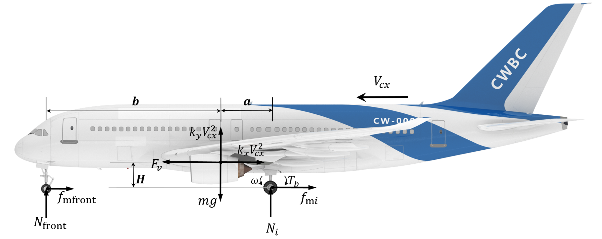
2.1. Aircraft Landing System Dynamics

Without loss of generality, in this paper, the aircraft body and landing gear are regarded as rigid bodies, and the earth is regarded as an inertial coordinate system. In addition, the curvature of the earth is ignored by [13]. Under this assumption, the dynamic model of the aircraft can be described by Equation (1), and the interaction of forces is shown in Figure 1. See

Table 1. Parameters for the aircraft model.

Name	Description
m	Aircraft mass
v	Aircraft longitudinal velocity
$T_0$	Engine residual thrust
$F_{xa}$	Aerodynamic drag
$F_y$	Aerodynamic lift
$F_s$	Parachute drag
$F_x$	Braking force
$F_{am}$	Support force of main landing gear
$F_{af}$	Support force of nose landing gear
n	Number of main wheels
$h_c$	Height of center of gravity
$h_s$	Distance between parachute drag line and gravity center
a	Distance between main wheel and gravity center
b	Distance between front wheel and gravity center
$\rho$	Air density
$C_x$	Aerodynamic drag coefficient
$C_y$	Aerodynamic lift coefficient
$C_{sx}$	Parachute drag coefficient
$S_x$	Aerodynamic drag coefficient
$S_y$	Aerodynamic lift coefficient
$S_{sx}$	Parachute area
$Kt$	Velocity coefficient of engine
$T_{0\_ini}$	Velocity coefficient of engine

for parameter descriptions.

$$m\dot{v}=T_0-F_{x}a-F_s-n{F}_x$$

(1)

$$F_y+F_{z}f+n{F}_{z}m=mg$$

(2)

$$F_{z}fb-n{F}_x{h}_c-n{F}_{z}ma+F_s{h}_s-T_0{h}_t=0$$

(3)

where

$$F_x=\frac{1}{2}\rho C_x{s}_x{v}^2,F_y=\frac{1}{2}\rho C_y{s}_y{v}^2,F_x=\frac{1}{2}\rho C_{sx}{s}_{sx}{v}^2,T_0=T_{0\_ini}+K_{t}v$$

The angular velocity of the braking wheel is described as follows:

$$J_w\dot{\omega }=-B_w\omega +F_{x}r-T_b$$

(4)

where $\omega$, $J_w$, and r are the wheel angular velocity, wheel moment of inertia, and wheel radius, respectively, while $B_w$ is the friction torque coefficient, and $T_b$ is the brake torque generated by the brake device [14].

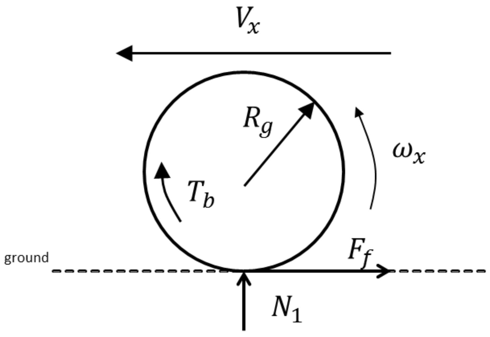
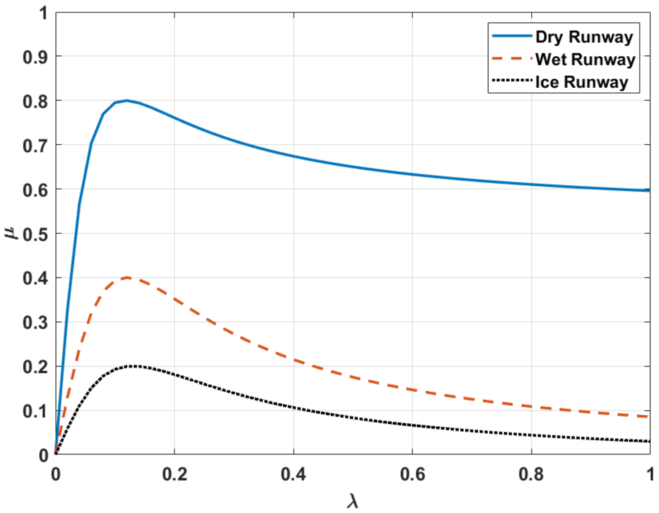
2.2. Aircraft Tire Dynamics

The friction characteristic between the tire and the ground is the main factor affecting the process of aircraft landing and braking. In fact, the bonding force between the tire and the road surface is the most important force that makes the aircraft decelerate. Moreover, the tires transfer the vertical load $F_z$ into longitudinal friction $F_x$, as illustrated in Figure 2. In fact, $F_x$ depends on a large number of features of the road, tire, and suspension. Most often, they can be described as follows:

$$F_x=f(F_{zm},\alpha ,\gamma ,\lambda )$$

(5)

The Pacejka model, represented in Equation (3), is perhaps the most well-known tire friction model [15]. This is because the model matches the experimental data well and is easy to implement. The expression of the tires has the following form:

$$f(F_{z}m;\alpha ;\gamma ;\lambda )=cos\left(C_{xt}arctan\left(B_{xt}\lambda \right)\right)F_{x0}$$

(6)

where the expressions of the different terms appearing in Equation (6) depend on $F_z,\alpha ,\gamma ,\lambda$, and several constant parameters, which are determined by the structural characteristics of the tire and can be easily identified from experimental data [15]. In this work, the aircraft is assumed to be symmetric during the braking process, and in the rest of this work, the design of the control algorithm is performed under the assumptions of small side slip and camber angles (i.e., $t=0$ and $\gamma =0$), which is to say that only longitudinal forces of the tire are of concern. Thus, Equation (4) can be simplified into the following:

$$F_x=F_z\mu \left(\lambda \right)$$

(7)

Based on the Pacejka model, the longitudinal coefficient between the tire and the ground has the following form [16,17]:

$$\mu \left(\lambda \right)=Dsin\left(Carctan\right(B\lambda \left)\right)$$

(8)

The parameters of the three most commonly used runway models are depicted in

Table 2. The parameters of the three most commonly used runway models.

Road Condition	B	C	D
Dry	14.0326	1.5344	0.8
Wet	8.2098	2.0192	0.4
Ice	7.201788	2.0875	0.2

, while $\mu -\lambda$ curves of the friction coefficient and wheel slip ratio are shown in Figure 3.

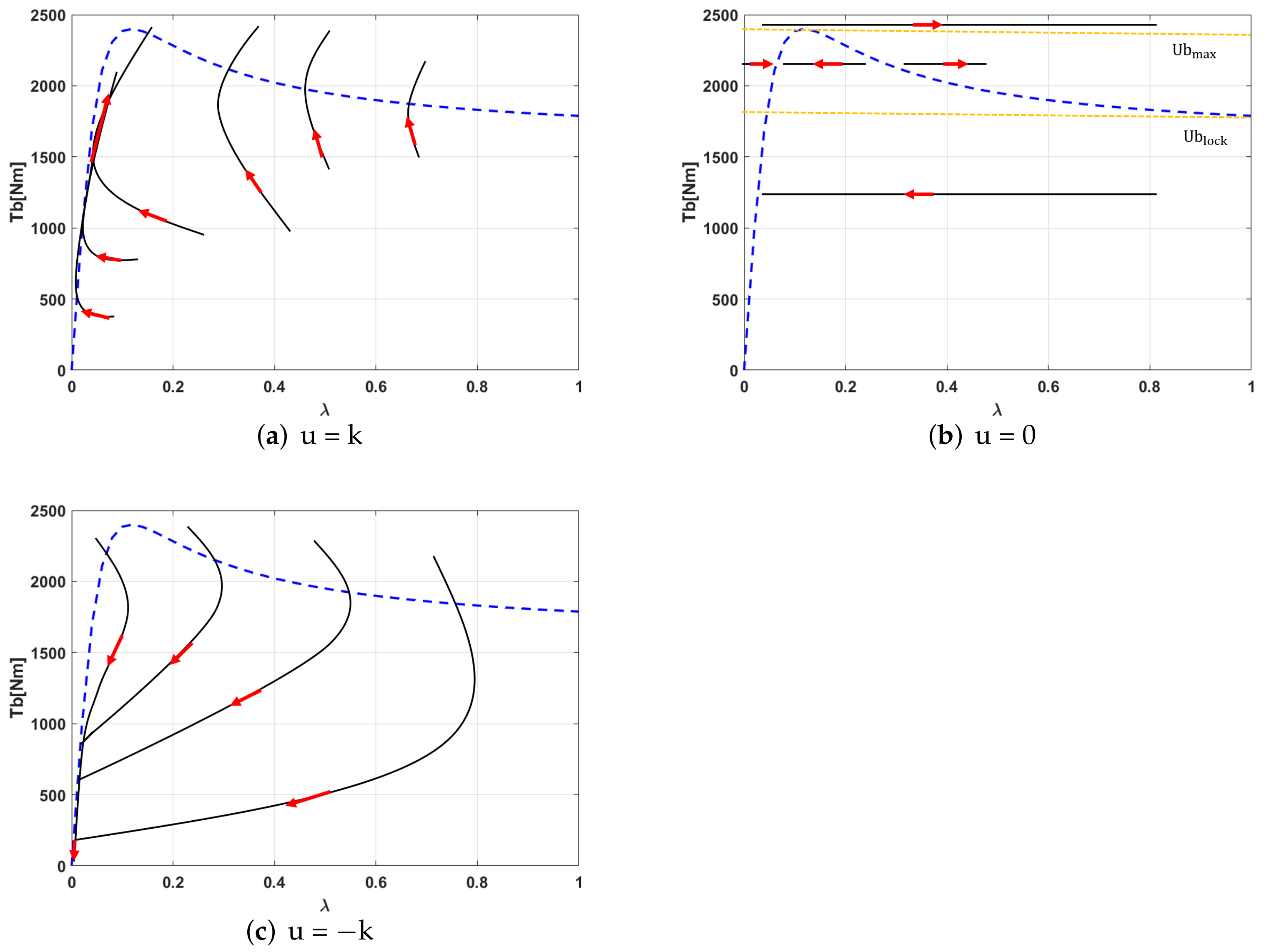
3. Problem Formulation

In this work, we only consider braking control (hence $v>\omega r$); thus, the slip rate can defined as:

$$\lambda =(v-r)/v$$

(9)

Substitute Equations (7) and (8) into Equations (1) and (2) yields the following:

$$\dot{v}=\frac{T_0-F_{xa}-F_s}{m}-\frac{\mu \left(\lambda \right)}{m}\frac{(mgb-F_{y}b+F_s{h}_s-T_0{h}_t)}{a+b+\mu (\lambda ,V_x)h_c}$$

(10)

$$\dot{\omega }=(B_w+F_{zm}r\mu \left(\lambda \right))/J_w-T_b/J_w$$

(11)

Taking the time derivative of Equation (9) yields:

$$\dot{\lambda }=-(r/v)\dot{\omega }+(r\omega /v^2)\dot{v}$$

(12)

Substituting Equations (10) and (11) into Equation (12) yields:

$$\dot{\lambda }=f\left(\lambda \right)+r/J_{w}v{T}_b$$

(13)

where $f\left(\lambda \right)=\frac{(1-\lambda )}{v}(\frac{(T_0-F_{x}a-F_s)}{m}-\frac{\mu \left(\lambda \right)}{m}\frac{(mgb-F_{y}b+F_s{h}_s-T_0{h}_t)}{(a+b+\mu \left(\lambda \right)h_c)})-\frac{r}{J_{w}v}[-B_w\omega +F_{zm}r\mu \left(\lambda \right)]$.

Under the assumption that aircraft speed v is a slowly varying parameter, and expressing v as $v=\omega r/(1-\lambda )$, the system dynamics can be given as follows:

$$\dot{\lambda }=-((1-\lambda )/J\omega )(\psi \left(\lambda \right)-Tb)$$

(14)

where $\omega >0$ and

$$\begin{array}{cc}\hfill \mathsf{\Psi }\left(\lambda \right)=& -B_w\omega +F_{zm}r\mu \left(\lambda \right)-\frac{J(1-\lambda )}{r}\left(\frac{\left(T_0-F_{xa}-F_s\right)}{m}-\frac{\left(\mu \right(\lambda \left)\right)}{m}\right.\hfill \\ \hfill & \left.\frac{\left(mgb-F_{y}b+F_s{h}_s-T_0{h}_t\right)}{\left(a+b+\mu \left(\lambda \right)h_c\right)}\right)\hfill \end{array}$$

(15)

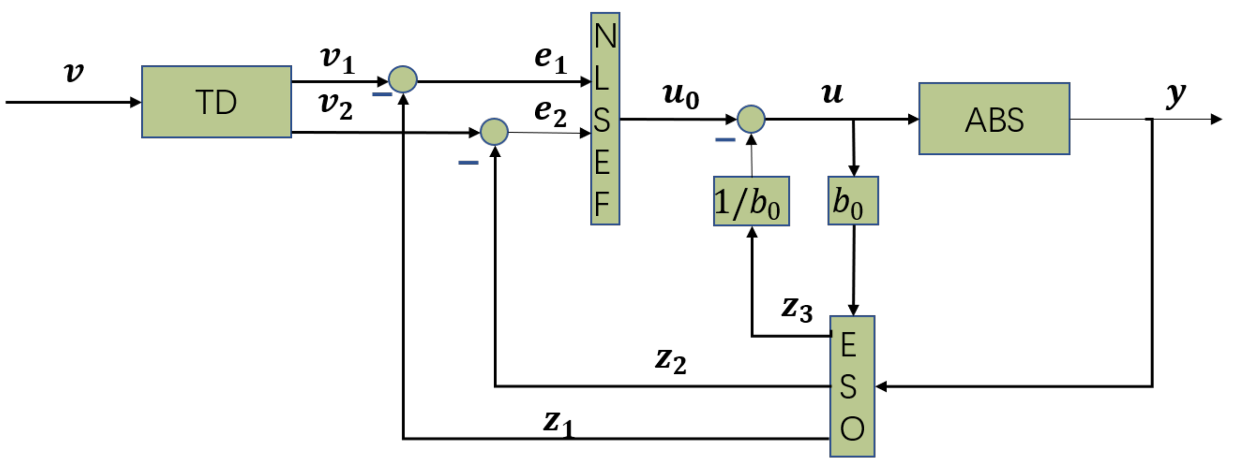
4. Controller Design

The main purpose of this work is to design a control law, so that the anti-skid braking system of the aircraft can be stabilized near the optimal value of the slip rate to improve the efficiency and safety of the braking process.

4.1. Design and Parameter Optimization of Aircraft Anti-Skid Braking Active Disturbance Rejection Controller

The performance of aircraft braking systems is mainly dependent on the tire/road characteristics and actuator dynamics. Accordingly, the main purpose of the control algorithm will be to maintain the system slip rate near optimal values, thus improving braking efficiency. To solve this problem, this work designs an active disturbance rejection controller, starting from the analysis of tire/road friction characteristics and system equilibrium.

Figure 4 is a schematic diagram of the balance point of the system when the control input of the controller is constant (i.e., $T_b=T_b^{ss}$). The system variable $\lambda$ exhibits equilibrium points, which can be seen in Figure 4:

(1) If $T_b^{ss}>{\lambda }_{max}\psi \left(\lambda \right)$, that is, if the brake torque is greater than the maximum friction value the tire can generate at the time, then the slip rate has a tendency of increasing, so the unique equilibrium point is ${\lambda }_{ss}=1$.

(2) If $T_b^{ss}<{\lambda }_{max}\psi \left(\lambda \right)$, then the system has at most three equilibria, namely ${\lambda }_1^{ss}=1$, ${\lambda }_2^{ss}={\lambda }_2$, and ${\lambda }_3^{ss}={\lambda }_3$, where ${\lambda }_2$ and ${\lambda }_3$ are the two possibly coincident solutions of $T_b^{ss}=\psi \left(\lambda \right)$, as shown in Figure 4. To facilitate the analysis of system dynamics with control action, in this section we assume the braking torque of the actuator as $T_b=Ku$. The system trajectories under control can be seen in Figure 5.

Where K = $-r$, 0, r. Therefore, the slip rate change rate concerning actuator dynamics yields the following second-order equation:

$$\left\{\begin{array}{c}\dot{\lambda }=-((1-\lambda )/J\omega )\left(\mathsf{\Psi }\left(\lambda \right)-T_b\right)\hfill \\ \dot{T_b}=u\hfill \end{array}\right.$$

(16)

Accordingly, the control system will maintain the wheel slip ratio around the acceptable values by generating a suitable value of variable r. To achieve this goal, this work designs an active disturbance rejection controller Figure 6.

(1) According to system dynamics, the input v of the controller is the desired slip rate, so we arrange the transient process of the controller as follows:

$$\left\{\begin{array}{c}{e}_{\lambda }=v_1-v\hfill \\ fh=fhan(e_{\lambda },v_2,r_0,h)\hfill \\ v_1=v_1+H{v}_2\hfill \\ v_2=v_2+Hfh\hfill \end{array}\right.$$

(17)

(2) Then, we track and estimate the states and disturbance of the system by output y and input v.

$$\left\{\begin{array}{c}e=z_1-y\hfill \\ fe=fal(e,0.5,\delta )\hfill \\ {fe}_1=fal(e,0.25,\delta )\hfill \\ z_1=z_1+h(z_2-{\beta }_{01}e)\hfill \\ z_2=z_2+h(z_3-{\beta }_{02}fe+b_{0}u)\hfill \\ z_3=z_3+h(-{\beta }_{03}{fe}_1)\hfill \end{array}\right.$$

(18)

(3) The nonlinear state error feedback is as follows:

$$\left\{\begin{array}{c}{e}_1=v_1-z_1\hfill \\ e_2=v_2-z_2\hfill \\ u_0={\beta }_{1}fal\left(e_1,{\alpha }_1,\delta \right)+{\beta }_{2}fal\left(e_2,{\alpha }_2,\delta \right)\hfill \end{array}\right.$$

(19)

(4) The disturbance compensation process is as follows:

$$u=u_0-\left(z_3\left(t\right)\right)/b_0$$

(20)

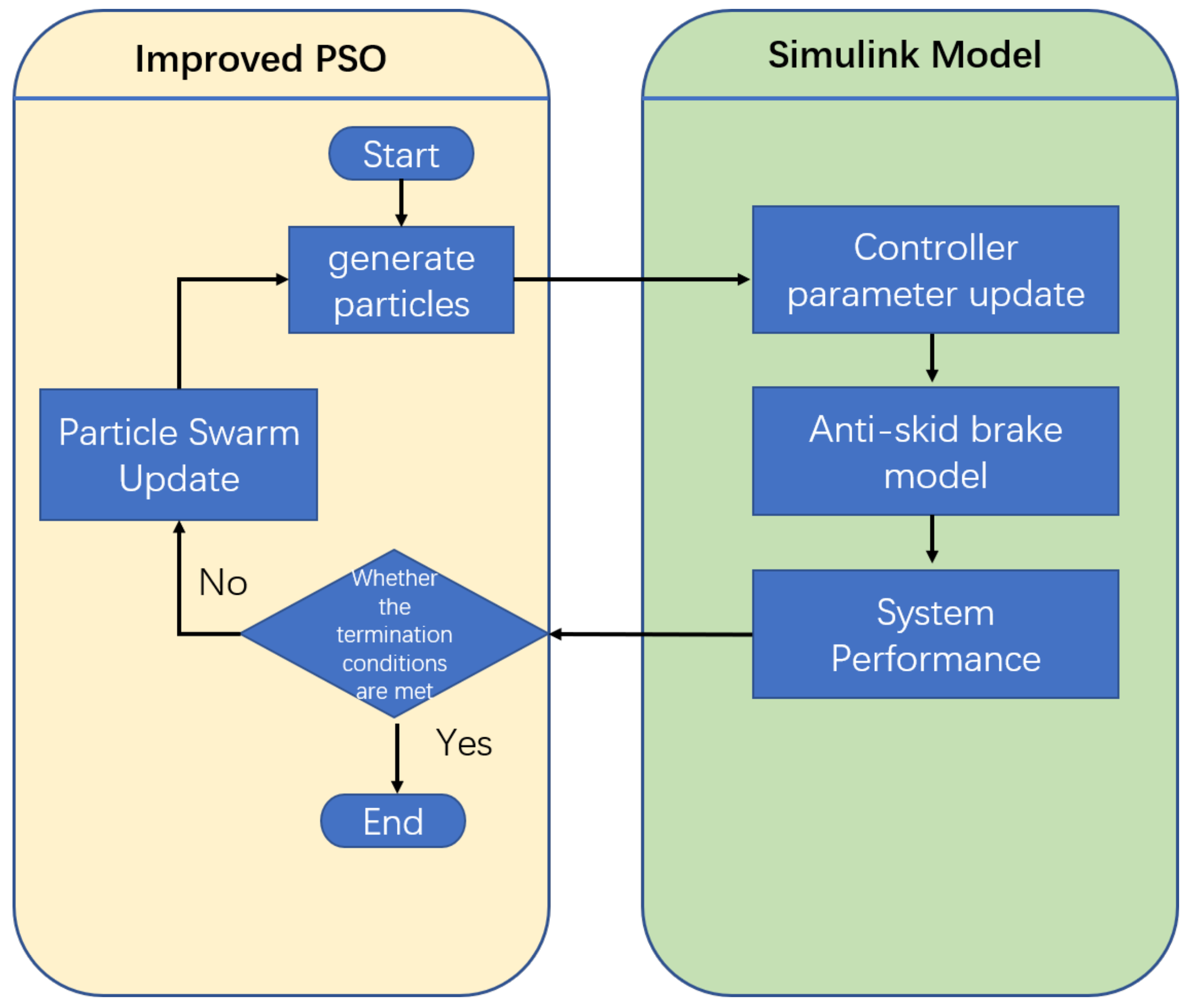
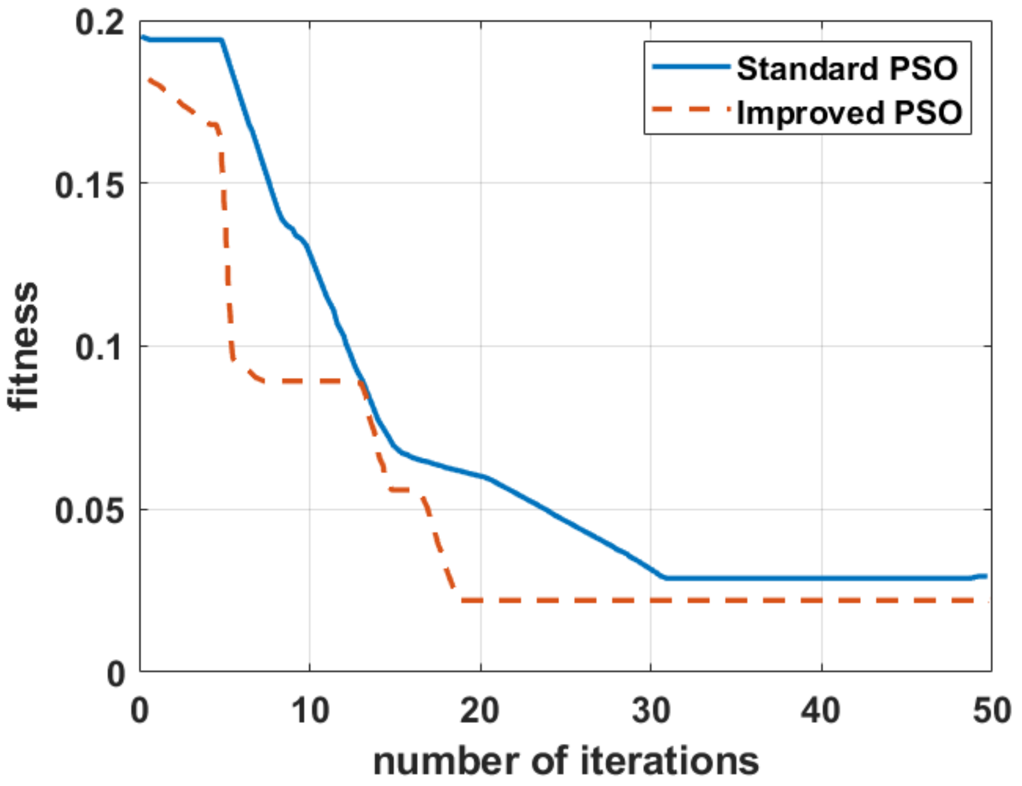
4.2. Optimization of Control Parameters Based on Improved Particle Swarm Optimization

Although it is easy to implement in industry, the parameter adjustment of ADRC is more complicated than other algorithms. There are more than ten parameters, and there is no specific standard for selecting parameters. The selection of parameters depends on the experience of the designer, so it can be time consuming, laborious, and limited in effect. In this paper, the improved PSO is used to adjust the parameters of the anti-skid braking active disturbance rejection controller. A flow chart of the particle swarm optimization is shown in Figure 7.

The basic PSO algorithm can be expressed as:

$$\left\{\begin{array}{c}{V}_{ij}(t+1)=V_{ij}\left(t\right)+c_1{r}_1\left(P_{ij}-X_{ij}\right)+c_2{r}_2\left(P_{gj}-X_{ij}\right)\hfill \\ X_{ij}(t+1)=X_{ij}\left(t\right)+V_{ij}(t+1)\hfill \end{array}\right.$$

(21)

For more on the basic particle swarm optimization algorithm, refer to the literature.

The basic particle swarm algorithm needs to adjust few variables, and it is simple and convenient to use. However, there are also shortcomings. The most prominent problem is that it is easy to converge prematurely, and the more the algorithm iterates later, the easier it is to converge prematurely. As researchers’ understanding of particle swarm optimization has continued to deepen, inertial weights have been proposed, which can represent the trend of particles’ past motion and expand the search space of particles. The size of the weight affects the search ability and the accuracy of the particle swarm. When the weight is increased, the algorithm focuses on the global search; when the inertia weight is reduced, the algorithm focuses on the local search accuracy. The standard particle swarm algorithm uses linearly decreasing weights. The principle is to use larger weights in the early stage, while in the later stages of the algorithm, the weights will be automatically adjusted to be linearly decreasing. The velocity formula after adjusting the inertia weight is as follows:

$$V_{ij}(t+1)=\omega V_{ij}\left(t\right)+c_1{r}_1\left(V_{ij}-X_{ij}\right)+c_2{r}_2\left(P_{gj}-X_{ij}\right)$$

(22)

where $\omega$ decreases linearly:

$$\omega ={\omega }_{\mathrm{start}}-\frac{{\omega }_{\mathrm{start}}-{\omega }_{\mathrm{end}}}{t_{max}}\times t$$

(23)

where ${\omega }_{\mathrm{start}}$ is the starting weight, ${\omega }_{\mathrm{end}}$ is the ending weight, ${\omega }_{\mathrm{start}}>{\omega }_{\mathrm{end}}$, and ${\omega }_{\mathrm{start}}$ eventually decays linearly to ${\omega }_{\mathrm{end}}$ as the iteration progresses. In the initial stage of the algorithm iteration, a larger inertia weight can prevent the particle harvesting speed from being too fast, resulting in prematurely obtaining a local optimal solution. In the later stage of the algorithm, the smaller inertia weight can improve the convergence accuracy of the algorithm. Usually, you can assume ${\omega }_{\mathrm{start}}=0.9$, and ${\omega }_{\mathrm{end}}=0.4$. In a standard particle swarm, linearly decreasing inertia weights are used, and the learning factors c1 and c2 are not improved. In this paper, a new form of inertia weight is selected on the basis of the standard particle swarm, and the learning factor of the particle swarm is readjusted. The following nonlinear functions are optimized, and the effects of different weight forms and learning factors on the optimization process are compared and analyzed.

For the comparison and simulation of linearly decreasing weight and adaptive adjustment weight, the form of the linearly decreasing weight is as follows:

$${\omega }_k={\omega }_{\mathrm{end}}+\left({\omega }_{\mathrm{start}}-{\omega }_{\mathrm{end}}\right)\left(1-\frac{k}{T}\right)$$

(24)

In the above formula, K is the current number of iterations, and T is the maximum number of iterations. The adaptive adjustment weights are as follows:

$$\omega =\left\{\begin{array}{cc}{\omega }_{min}-\left({\omega }_{max}-{\omega }_{min}\right)\frac{f-f_{min}}{\overline{f}-f_{min}}\hfill & f\le \overline{f}\hfill \\ {\omega }_{max}\hfill & f>\overline{f}\hfill \end{array}\right.$$

(25)

In the above formula, f is the current fitness value, $\overline{f}$ is the average fitness value, and $f_{\min }$ is the minimum fitness value, while ${\omega }_{\max }$ and ${\omega }_{\min }$ are the maximum and minimum weights, respectively. This paper improves the standard particle swarm. The concept behind the improvement is to adjust the inertia weight and the learning factor of the particle swarm, and to introduce the natural selection mechanism. The steps for obtaining the minimum value problem of the improved particle swarm are as follows:

A. Set the size of the particle swarm, that is, how many particles there are in the swarm, and set the starting position and speed of the particles. Set the maximum and minimum values of the learning factor. Specify the maximum and minimum weights.

B. Calculate the fitness of each particle. Store the particle position and fitness value at the moment in the individual extreme value in $P_{best}$. Among all the individual extreme values, the particle with the lowest fitness is selected by comparison. Store the particle’s position and fitness value in the global extremum $g_{best}$.

C. Use the synchronous learning factor to update the speed of the particle:

$$\left\{\begin{array}{c}{c}_1=c_2=c_{max}-\left(c_{max}-c_{min}\right)\frac{t}{T}\hfill \\ V_{ij}(t+1)=\omega V_{ij}\left(t\right)+c_1{r}_1\left(P_{ij}-X_{ij}\right)+c_2{r}_2\left(P_{gj}-X_{ij}\right)\hfill \\ X_{ij}(t+1)=X_{ij}\left(t\right)+V_{ij}(t+1)\hfill \end{array}\right.$$

(26)

D. Perform adaptive weights adjustment:

$$\omega =\left\{\begin{array}{cc}{\omega }_{min}-\left({\omega }_{max}-{\omega }_{min}\right)\frac{f-f_{min}}{\overline{f}-f_{min}}\hfill & f\le \overline{f}\hfill \\ {\omega }_{max}\hfill & f>\overline{f}\hfill \end{array}\right.$$

(27)

In the above formula, f is the current fitness value, $\overline{f}$ is the average fitness value, and $f_{\min }$ is the minimum fitness value, while ${\omega }_{\max }$ and ${\omega }_{\min }$ are the maximum and minimum weights, respectively. It can be seen from Figure 4 that the optimization process is as follows: First, a particle swarm is generated, and the swarm particles are assigned to the parameters $k_1$, $k_2$, ${\beta }_1$, ${\beta }_2$, and ${\beta }_3$. Then, the model of the control system is run to obtain the performance index corresponding to the set of controller parameters. Then, the performance index is transferred to the particle swarm as the fitness value of the current particle. Finally, it is judged whether the termination condition is met. The error performance index adopts the ITAE criterion, so the fitness function form of the particle swarm algorithm is as follows:

$$\mathrm{fitness}={\int }_0^{\infty }t\left|e\left(t\right)\right|dt$$

(28)

The tuned parameters are the observer gains ${\beta }_1$, ${\beta }_2$, and ${\beta }_3$, and the gain coefficients $k_1$ and $k_2$ in the control law. Therefore, the particle swarm algorithm is initialized to 5 dimensions, the initial scale is 50 particles, the termination condition is 50 iterations, the inertia weights are ${\omega }_{\max }=0.9$ and ${\omega }_{\min }=0.36$, and the learning factors are $c_{\max }=2.2$ and $c_{\min }=0.8$. The initialization parameters are shown in

Table 3. Initialization parameter of particle swarms.

Parameter	${\mathit{k}}_1$	${\mathit{k}}_2$	${\mathit{\beta }}_1$	${\mathit{\beta }}_2$	${\mathit{\beta }}_3$
Position upper limit	300	300	200	1000	4000
Position lower limit	0.5	0.5	50	50	50
Velocity upper limit	1	1	2	5	5
Velocity lower limit	−1	−1	−2	−5	−5

. The fitness curves of the standard particle swarm and the improved particle swarm algorithm are shown in Figure 8. We can see that the improved particle swarm algorithm has a faster convergence speed and better optimization effect (the fitness value is smaller).

4.3. Stability Analysis

Stability may be the most important indicator of a control system, especially for aircraft anti-skid braking systems. The stability of ADRC is also one of the key points of academic attention, and many landmark achievements have emerged [18,19,20,21]. Stability analysis of an ADRC system was performed via the describing function method by D. Wu et al. [22,23]. In addition, time domain convergences of the ADRC system were proven [22,24]. However, for typical nonlinear ADRC systems, there is still no suitable Lyapunov function, and there are many restrictions on the parameters, which makes the method difficult to apply. In this work, we adapt the absolute stability method to prove the stability of the ADRC designed for aircraft anti-skid braking system. Moving forward, we work under the following assumptions:

(A1) The input of TD is 0 (i.e., $v=0$); hence, the output value of TD $v_1$ is also zero.

(A2) Nonlinear state error feedback is converted to linear state error feedback by first-order approximation.

$$u=\sum _{i=1}^n{k}_i{z}_i-z(n+1)/b$$

(29)

(A3) The nonlinear function $\phi \left(x\right)$ is chosen in the design of ESO, such that for all $x_0,x\phi \left(x\right)>0$, and $\phi F\left({\mu }_1,{\mu }_2\right)$ The following two requirements are introduced: $\phi \left(0\right)=0$; $\exists 0<{\mu }_1<{\mu }_2$ for $\forall x0,{\mu }_1{x}^2<x\phi \left(x\right)<{\mu }_2{x}^2$ (i.e., $\phi \left(x\right)F(0,+]$). Then, the output of ESO can be rewritten as:

$$\left\{\begin{array}{c}{\dot{z}}_1=z_2-{\beta }_1\phi \left(z_1-y\right)\\ ⋮\\ {\dot{z}}_n=z_{(n+1)}-{\beta }_n\phi \left(z_1-y\right)+bu\\ \left.\dot{z}(n+1)=-(n+1)\phi \left(z_1-y\right)\right)\end{array}\right.$$

(30)

(A4) Let the object system under control be a linear time-invariant system. Then, the state space form of the controlled object can be expressed as:

$$\left\{\begin{array}{c}{\dot{x}}_1=x_2\hfill \\ ⋮\hfill \\ {\dot{x}}_n=-a_n{x}_1-a_{(n-1)}{x}_2-\dots -a_1{x}_n+bu\hfill \\ \dot{z}(n+1)=-(n+1)\phi \left(z_1-y\right))\hfill \end{array}\right.$$

(31)

Substituting Equation (29) into Equation (31) yields:

$$\left\{\begin{array}{c}\dot{X}=A_{11}X+A_{12}Z+a_{13}z(n+1)\hfill \\ y=x_1\hfill \end{array}\right.$$

(32)

where $X={\left[x_1,x_2,\dots ,x_n\right]}^T, Z={\left[z_1,z_2,\dots ,Z_n\right]}^T, a_{13}={[0,\dots ,0,-1]}^T\in R^n$

$$A_{11}=\left[\begin{array}{ccccc}0& 1& 0& \cdots & 0\\ 0& 0& 1& 0& 0\\ ⋮& ⋮& ⋮& \ddots & ⋮\\ 0& 0& 0& \cdots & 1\\ -a_n& -a_{n-1}& -a_{n-2}& \cdots & a_1\end{array}\right]A_{12}=\left[\begin{array}{ccc}0& \cdots & 0\\ 0& \cdots & 0\\ ⋮& \ddots & ⋮\\ 0& \cdots & 0\\ -b{k}_1& \cdots & -b{k}_n\end{array}\right]$$

Substituting Equation (29) into Equation (30), yields:

$$\left\{\begin{array}{c}\dot{X}=A_{11}X+A_{12}Z+a_{13}z(n+1)\hfill \\ \dot{Z}=A_{22}Z+b_{2}u\hfill \\ \dot{z}(n+1)=\beta (n+1)u\hfill \\ u=-\phi \left(y\right)\hfill \\ y=c_1^{T}X+c_2^{T}Z\hfill \end{array}\right.$$

(33)

Let $Y=A_{11}X+a_{13}z(n+1), z{(n+1)}^{\prime }=z(n+1)/{\beta }_{(n+1)}$, and we get:

$$\left\{\begin{array}{c}\dot{Y}=A_{11}Y+A_{11}{A}_{12}Z+a_{13}\beta (n+1)u\hfill \\ \dot{Z}=A_{22}Z+b_{2}u\hfill \\ \dot{z}(n+1)=u\hfill \\ u=-\phi \left(y\right)\hfill \\ y=c_1^T{A_{11}}^{-1}Y+c_2^{T}Z-c_1^T{A_{11}}^{-1}{a}_{13}\beta (n+1)z{(n+1)}^{\prime }\hfill \end{array}\right.$$

(34)

Equation (34) conforms to one standard form of the first critical situation of absolute stability [25], that is,

$$\left\{\begin{array}{c}\dot{x}=Ax+bu\hfill \\ \epsilon =u\hfill \\ u=-\phi \left(y\right)\hfill \\ y=c^{T}x=p\epsilon \hfill \end{array}\right.$$

(35)

where $A=\left[\begin{array}{cc}{A}_{11}& A_{12}{A}_{12}\\ 0& A_{22}\end{array}\right]$

$b=\left[\begin{array}{c}{a}_{13}{\beta }_{n+1}\\ b_2\end{array}\right]$

$C^T=\left[\begin{array}{cc}{c}_1^T{A}_{11}{}^{-1}\hfill & c_2^T\hfill \end{array}\right]$

$\rho =-c_1^T{A}_{11}^{-1}{a}_{13}\beta (n+1)=\beta (n+1)/a_n$

Theorem 1.

The necessary condition of absolute stability of Equation (35) in regard to $F(0;+1]$ is $Re\lambda \left(A\right)<0$; $\rho >0$ [26]. If the linear time-invariant object mentioned above is asymptotically stable (i.e., all the eigenvalues of $A_{11}$ have a negative real part), at the same time we can ensure all the eigenvalues of $A_{12}$ have a negative real part by choosing an appropriate value of parameter ki. Hence, all the eigenvalues of A have a negative real part; thus, we get the following theorem.

Theorem 2.

The necessary conditions of absolute stability of the ADRC system equation (i.e., Equation (34)) are that the linear time-invariant object is asymptotic and the control parameters are positive, while at the same time ensuring that $Re\lambda \left(A_{22}\right)<0$. Consider now the candidate Lyapunov function: $U(x,y)=x^{T}Px+\alpha {\left(y-c^{T}x\right)}^2+\beta {\int }_0^y\phi \left(y\right)dy$. If P is chosen as positive definite matrix, then function $U(x,y)$ is a zero solution. Take the time derivative of Equation (36) and substitute Equation (35) into the derivative equation $\dot{U}(x,y)=-x^{T}Qx-2d^{T}x\phi \left(y\right)+\gamma {\phi }^2\left(y\right)+2\alpha \rho y\phi \left(y\right)$, where $Q=-PA-A^{T}P,d=Pb-\left(\alpha \rho c+1/2\beta A^{T}c\right),\gamma =\beta \left(\rho +c^{T}b\right)$ as $y\phi \left(y\right)>0,\rho ={\beta }_{(n+1)}/a_n>0$, provided $\alpha \ge 0$, and the former three terms of Equation 30 are negative quadratic forms of x and φ. Then, $\dot{U}$ is negative, thus guaranteeing the global asymptotic stability of Equation (35).

Lemma 1.

Let $Q=Q^T\in R^n,\gamma \in R,d\in R^n,C^T=\left[\begin{array}{cc}Q& d\\ d^T& \gamma \end{array}\right]$ be positive definite if and only one of the following two conditions hold:

(1) $Q>0,\gamma -d^T{Q}^{-1}d>0$;

(2) $\gamma >0,Q-\frac{1}{\gamma }d{d}^T>0$;

Theorem 3.

Suppose that λ and β are non-negative real numbers that are not equal to zero at the same time, and P is a positive definite matrix that can make Q and d satisfy the conditions of Lemma 1. If this is the case, then the zero solution, according to $F(0;+1]$ of Equation (35), is absolute stable (Bochun Feng, Shumin Fei. 1990).

Theorem 4.

Suppose that α and β are non-negative real numbers that are not equal to zero at the same time. This makes $T\left(s\right)=(2\alpha \rho +\beta S)W\left(s\right)$ a positive real function, where $W\left(s\right)=cT(sI-A)-1b+\rho s$ is the transfer function of the system represented in Equation (35). Moreover, two additional factors need to be met: (1) T(s) has at least one negative real part pole; (2) when $\alpha =0$ for all $0<ϵ<+1$, the linearized system $\varphi \left(y\right)=ϵy$ is asymptotically stable. Then, the zero solution of system Equation (30), according to $F(0;+1]$, is absolute stable. As for the aircraft anti-skid braking system, according to the first approximation, Equation (16) can be approximated as:

$$\left\{\begin{array}{c}{\dot{x}}_1=x_2\hfill \\ {\dot{x}}_2=-a_1{x}_1-a_2{x}_2+g\left(x_1,x_2\right)+bu\hfill \\ y=x_1\hfill \end{array}\right.$$

(36)

where $x_1=\lambda ,x_2=-((1-\lambda )/J_w\omega )\left(\mathsf{\Psi }\left(\lambda \right)-T_b\right)$, and term g$\left(x_1,x_2\right)$ only contains terms higher than one degree of $x_i$.

Through transformation we can get the following:

$$\left\{\begin{array}{c}\dot{X}=A_{11}X+A_{12}Z+a_{13}{z}_{n+1}+a_{14}g\left(Y\right)\hfill \\ \dot{Z}=A_{22}Z+b_{2}u\hfill \\ {\dot{z}}_{n+1}={\beta }_{n+1}u\hfill \\ u=-\phi \left(y\right)\hfill \\ y=c_1^{\mathrm{T}}X+c_2^{\mathrm{T}}Z\hfill \end{array}\right.$$

(37)

Comparing this with Equation (35), the only difference is that Equation (37) has a nonlinear function item $g\left(Y\right)$, and $g\left(Y\right)$ only contains items higher than one degree. Thus, we can draw a conclusion that is similar to that of the first approximation theorem [27] (i.e., Theorem 5).

Theorem 5.

If the zero solution of the linear control object system represented in Equation (35) is absolute stable, then the zero solution of the nonlinear control object (aircraft anti-skid braking system) Equation (37) is asymptotically stable.

Proof. 

If the zero solution of Equation (35) is absolute stable, consider the candidate Lyapunov function:

$$\begin{array}{cc}\hfill \dot{U}(x,y)=& -x^{T}Qx-2d^{T}x\phi \left(y\right)-\gamma {\phi }^2\left(y\right)-2\alpha \rho y\phi \left(y\right)\hfill \\ \hfill & +2x^{T}P{G}^{,}\left(x\right)+\beta c^T{G}^{\prime }\left(x\right)\phi \left(y\right)\hfill \end{array}$$

(38)

where $G^{\prime }\left(x\right)=\left[\begin{array}{c}{a}_{14}^{\prime }{g}^{\prime }\left(Y\right)\\ 0\end{array}\right]$ only contains items higher than one degree of x, and the definitions of $Q,d$ are given by Equation (32). According to Lemma 1, $M=\left[\begin{array}{cc}Q& d\\ d^T& \gamma \end{array}\right]$ is positive definite, and as $G^{\prime }\left(x\right)$ only contains items higher than one degree of x, the sign of $\dot{U}(x,y)$ around the neighborhood of the origin only depends on the situation of M (i.e., negative definite). Thus, Equation (35) of the aircraft anti-skid braking system with ADRC is origin asymptotically stable. □

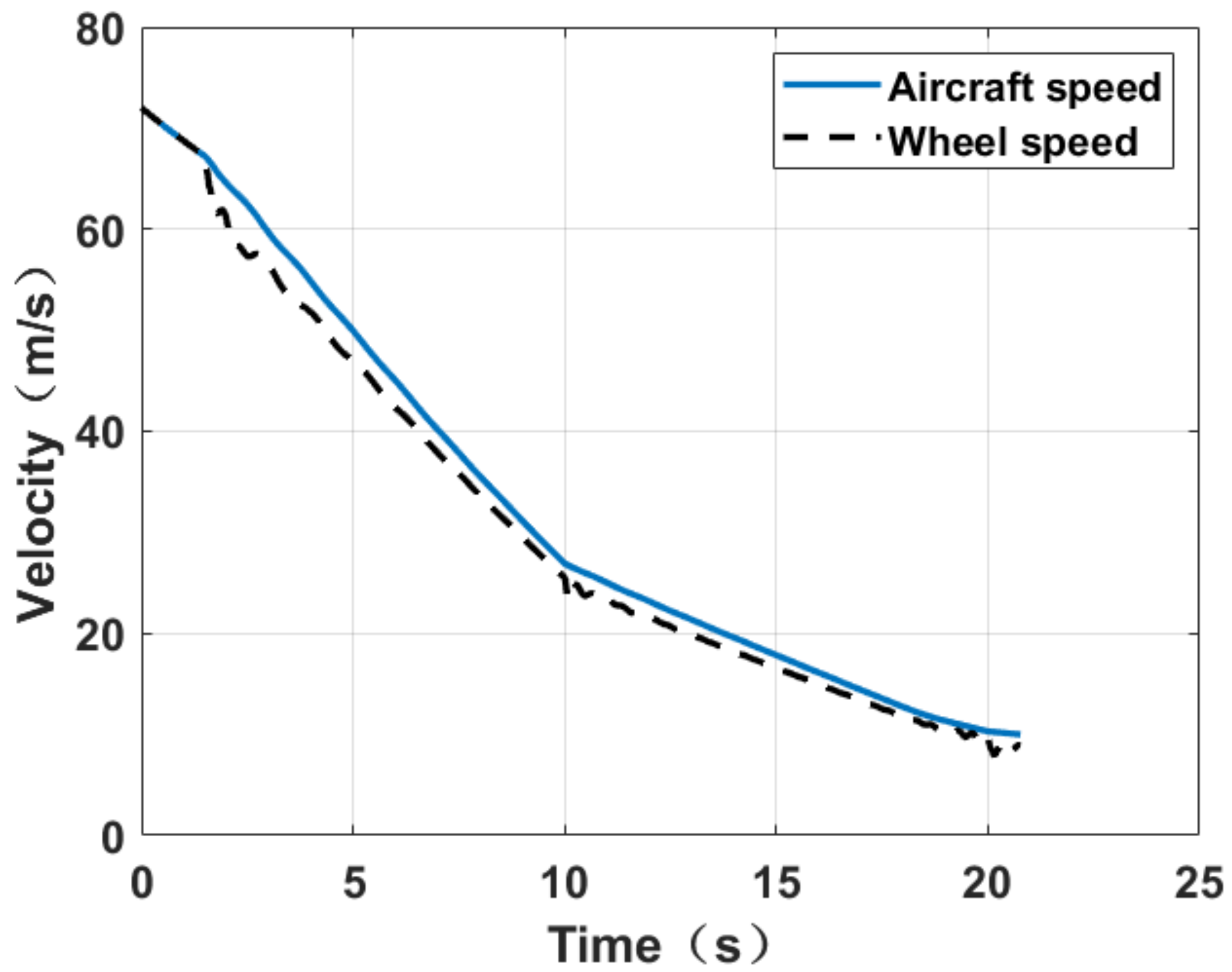
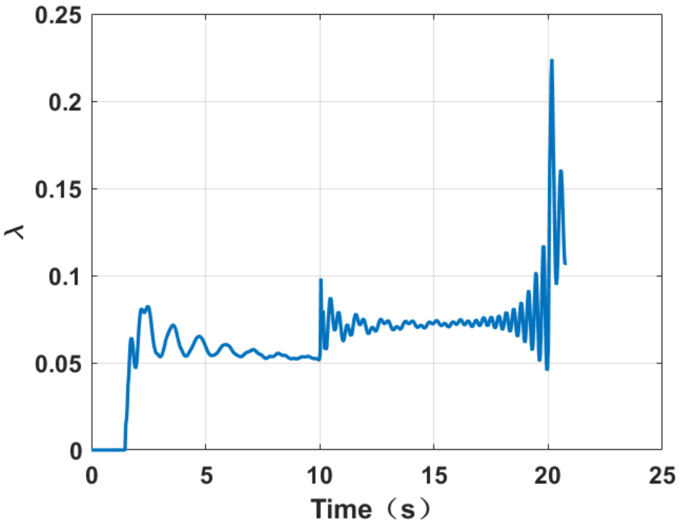
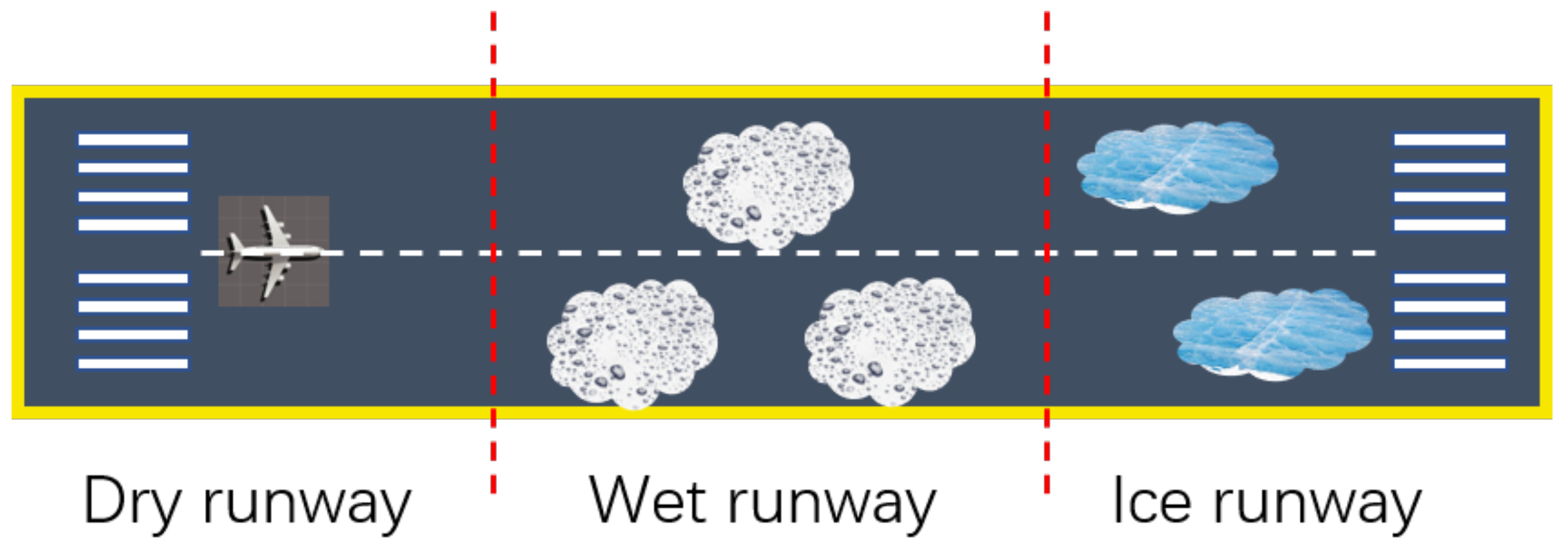
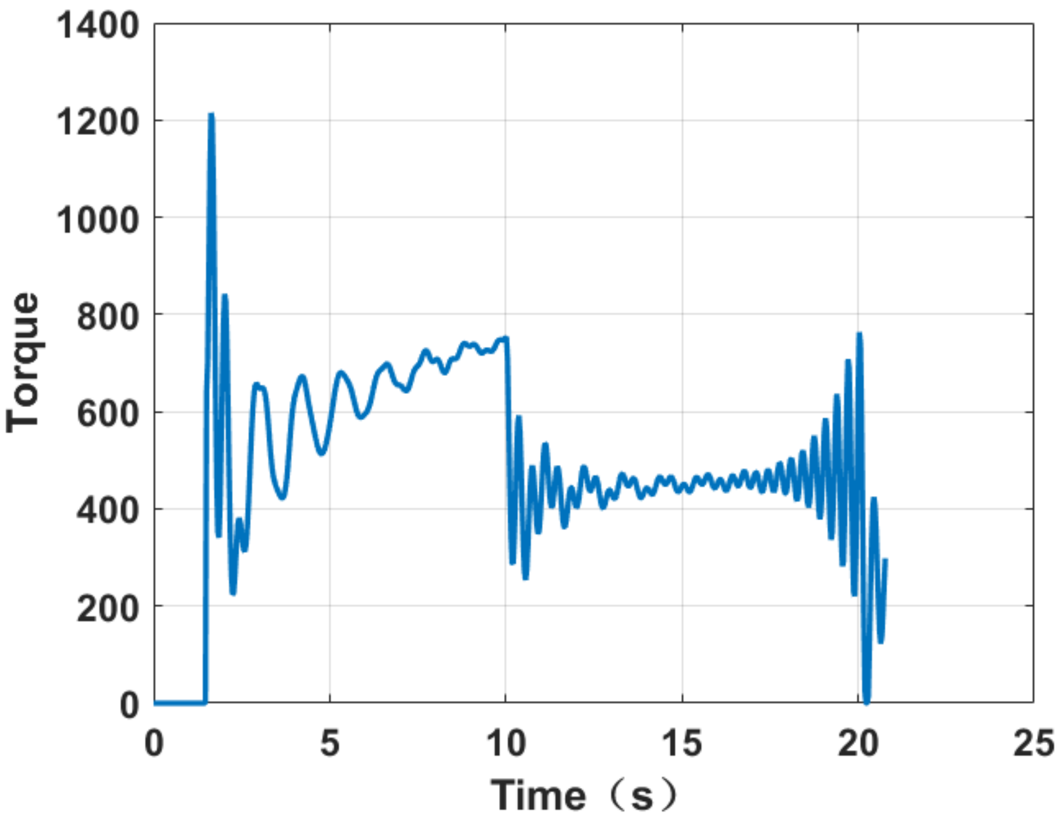
5. Simulation Study for Hybrid Runway Conditions

The performance of the algorithm proposed in this paper is verified by an aircraft anti-skid semi-physical simulation platform Figure 9.

Without loss of generality, we choose the mixed runway case as the simulation case for the proposed controller. The mixed runway layout is shown in Figure 10.

In this test, the initial speed of the anti-skid braking process is 72 m/s, and the failure speed is 7 m/s. Aircraft speed and tire speed are two important variables in the process of anti-skid braking, and they are also two dynamic characteristics to be considered in the design of the controller. The speed at which the body speed decreases to a large extent represents the braking efficiency of the anti-skid controller, and the difference between the tire speed and the body speed can roughly reflect the degree of tire slippage. If deep skidding occurs at high speed, it may lead to a tire blowout phenomenon, and this is an important problem that needs to be prevented in the design of the anti-skid controller.

As can be seen from Figure 11, under the control of the controller designed in this paper, the speed of the aircraft body and the wheel speed both drop steadily, and there is no deep skid phenomenon. When the runway changes, the controller can quickly perform anti-skid action to prevent wheel lock caused by the instantaneous reduction of ground friction, which reflects a good control effect.

Figure 12 is a graph of the system slip rate. The slip rate is the most important variable in the anti-skid control, because the slip rate is the most important factor affecting the ground bond coefficient. Generally speaking, 0.08–0.12 means that the system slip rate is relatively good. In this interval, the system stability is better, and the ground friction force utilization rate is higher. It can be seen from Figure 12 that under the control of the controller in this paper, the system slip rate can be maintained in the range of 0.08–0.12 most of the time, and there is no deep slip phenomenon during the whole braking process.

Figure 13 is a graph of the braking torque of the system. It can be seen that at the moment of runway switching (10 s, 20 s), the torque output by the controller can be adjusted quickly, because the runway is set to switch from a high-coefficient runway to a ground-coupling coefficient runway, so the controller quickly decompresses when the runway is switched, which avoids the problem of deep skidding and reflects the good adaptability to the runway state.

6. Conclusions

ADRC is a very high-quality approach for the manipulation and disturbance rejection of nonlinear systems. In this work, ADRC is designed to control the anti-skid braking progress of aircraft, and in order to better adjust the controller parameters, this paper also proposes an improved particle swarm optimization algorithm. It can be seen from Figure 8 that compared with the ordinary particle swarm algorithm, the improved particle swarm algorithm shows a faster convergence speed and better fitness.

This paper also proves the stability of the designed controller based on the Lyapunov method. The proposed algorithm was tested on an aircraft anti-skid braking semi-physical platform, and the result showed that the ADRC controller keeps the system operating in a stable region without deep skidding. Moreover, the tracking error of the adhesion coefficient converges to a small neighborhood around zero for each simulation.

References

1. Jiao, Z.; Wang, Z.; Sun, D.; Liu, X.; Shang, Y.; Wu, S. A novel aircraft anti-skid brake control method based on runway maximum friction tracking algorithm. Aerosp. Sci. Technol. 2021, 110, 106482. [Google Scholar] [CrossRef]
2. Du, C.; Li, F.; Yang, C.; Shi, Y.; Liao, L.; Gui, W. Multi-Phase-Based Optimal Slip Ratio Tracking Control of Aircraft Antiskid Braking System via Second-Order Sliding Mode Approach. IEEE-ASME Trans. Mechatron. 2021, 27, 823–833. [Google Scholar] [CrossRef]
3. Tanelli, M.; Astolfi, A.; Savaresi, S.M. Robust nonlinear output feedback control for brake by wire control systems. Automatica 2008, 44, 1078–1087. [Google Scholar] [CrossRef]
4. Johansen, T.A.; Petersen, I.; Kalkkuhl, J.C.; Lüdemann, J. Gain-scheduled wheel slip control in automotive brake systems. IEEE Trans. Control. Syst. Technol. 2003, 11, 799–811. [Google Scholar] [CrossRef] [Green Version]
5. Qiu, Y.; Liang, X.; Dai, Z. Backstepping dynamic surface control for an anti-skid braking system. Control Eng. Pract. 2015, 42, 140–152. [Google Scholar] [CrossRef]
6. Radac, M.B.; Precup, R. Data-driven model-free slip control of anti-lock braking systems using reinforcement Q-learning. Neurocomputing 2018, 275, 317–329. [Google Scholar] [CrossRef]
7. Radac, M.B.; Precup, R.; Roman, R.C. Anti-lock braking systems data-driven control using Q-learning. In Proceedings of the 2017 IEEE 26th International Symposium on Industrial Electronics (ISIE), Edinburgh, UK, 19–21 June 2017; pp. 418–423. [Google Scholar]
8. Qi, X.; Li, J.; Xia, Y.; Gao, Z. On the Robust Stability of Active Disturbance Rejection Control for SISO Systems. Circuits Syst. Signal Process. 2017, 36, 65–81. [Google Scholar] [CrossRef]
9. Chen, Z.; Zong, X.; Tang, W.; Huang, D. Design of rapid exponential integral nonlinear tracking differentiator. Int. J. Control. 2021, 1–8. [Google Scholar] [CrossRef]
10. Han, J. From PID to Active Disturbance Rejection Control. IEEE Trans. Ind. Electron. 2009, 56, 900–906. [Google Scholar] [CrossRef]
11. Qu, J.; Xia, Y.; Shi, Y.; Cao, J.; Wang, H.; Meng, Y. Modified ADRC for Inertial Stabilized Platform with Corrected Disturbance Compensation and Improved Speed Observer. IEEE Access 2020, 8, 157703–157716. [Google Scholar] [CrossRef]
12. Merino, J.S.; Castro, M.D.; Masi, A. An Application of Active Disturbance Rejection Control to Stepper Motors with Field Oriented Control. In Proceedings of the 2021 22nd IEEE International Conference on Industrial Technology (ICIT), Valencia, Spain, 10–12 March 2021; Volume 1, pp. 142–147. [Google Scholar]
13. Kou, Y.; Yu-Ren, L.I.; Liang, B. Design of Aircraft Electrical Integrated Test Management System Based on LabVIEW. Mod. Electron. Tech. 2011, 34, 124–127. [Google Scholar]
14. Zhang, X.; Lin, H. Backstepping Adaptive Neural Network Control for Electric Braking Systems of Aircrafts. Algorithms 2019, 12, 215. [Google Scholar] [CrossRef] [Green Version]
15. Pacejka, H.B. Tire and Vehicle Dynamics; Elsevier: Amsterdam, The Netherlands, 2012. [Google Scholar]
16. Kadir, Z.A.; Bakar, S.A.A.; Samin, P.M.; Hudha, K.; Harun, M.H. A new approach in modelling of hitch joint of a tractor semi-trailer using virtual Pacejka tyre model. Int. J. Heavy Veh. Syst. 2021, 28, 262. [Google Scholar] [CrossRef]
17. Cabrera, J.A.; Castillo, J.J.; Pérez, J.; Velasco, J.M.; Guerra, A.J.; Hernández, P. A Procedure for Determining Tire-Road Friction Characteristics Using a Modification of the Magic Formula Based on Experimental Results. Sensors 2018, 18, 896. [Google Scholar] [CrossRef] [Green Version]
18. Chen, H.; Sun, X.; Xu, S.; Wang, Y. Robust Stabilization of Extended Nonholonomic Chained-Form Systems with Dynamic Nonlinear Uncertain Terms by Using Active Disturbance Rejection Control. Complexity 2019, 2019, 1365134. [Google Scholar] [CrossRef]
19. Wang, Q.; Ran, M.; Dong, C. On Finite-Time Stabilization of Active Disturbance Rejection Control for Uncertain Nonlinear Systems. Asian J. Control 2018, 20, 415–424. [Google Scholar] [CrossRef] [Green Version]
20. Jie, L.; Qi, X.; Xia, Y.; Ma, D.; Xu, Y. On the absolute stability of nonlinear ADRC for SISO systems. In Proceedings of the 2015 34th Chinese Control Conference (CCC), Hangzhou, China, 28–30 July 2015. [Google Scholar]
21. Sun, Z.; Zhou, J.; Ling, Y.; Xie, X.; Yu, Y.; Sun, Z. Designing and application of modified SSA based ADRC controller for overhead crane systems. Int. J. Intell. Robot. Appl. 2022, 1–18. [Google Scholar] [CrossRef]
22. Wu, D.; Chen, K. Frequency-Domain Analysis of Nonlinear Active Disturbance Rejection Control via the Describing Function Method. IEEE Trans. Ind. Electron. 2013, 60, 3906–3914. [Google Scholar] [CrossRef]
23. Wu, D.; Chen, K. Limit cycle analysis of active disturbance rejection control system with two nonlinearities. ISA Trans. 2014, 53, 947–954. [Google Scholar] [CrossRef]
24. Li, J.; Qi, X.; Xia, Y.; Gao, Z. On asymptotic stability for nonlinear ADRC based control system with application to the ball-beam problem. In Proceedings of the 2016 American Control Conference (ACC), Boston, MA, USA, 6–8 July 2016; pp. 4725–4730. [Google Scholar]
25. Churilov, A.N. On an Application of the Absolute Stability Theory to Sampled-Data Stabilization. Math. Probl. Eng. 2018, 2018, 3169609. [Google Scholar] [CrossRef] [Green Version]
26. Grabowski, P. Absolute stability criteria for infinite-dimensional discrete Lur’e systems with application to loaded distortionless electric RLCG-transmission line. J. Differ. Equ. Appl. 2013, 19, 304–331. [Google Scholar] [CrossRef]
27. Jager, D. Nonlinear Control System Analysis and Design with Maple. Available online: https://pure.tue.nl/ws/files/4290655/604064.pdf (accessed on 15 March 2022).
Figure 1. Force analysis of fuselage.
Algorithms 15 00158 g001
Figure 2. Aircraft landing roll force.
Algorithms 15 00158 g002
Figure 3. Relationship between adhesion coefficient μ and slip rate λ .
Algorithms 15 00158 g003
Figure 4. Equilibrium points for aircraft anti-skid braking model.
Algorithms 15 00158 g004
Figure 5. System trajectories of states λ and T b when K = r (a), K = 0 (b), and K = r (c).
Algorithms 15 00158 g005
Figure 6. The structure of the ADRC.
Algorithms 15 00158 g006
Figure 7. Flow chart of particle swarm optimization.
Algorithms 15 00158 g007
Figure 8. Particle swarm algorithm fitness value change curve.
Algorithms 15 00158 g008
Figure 9. Semi-physical simulation platform of anti-skid braking system: (a) electrical console; (b) hydraulic pump and piping; (c) overall configuration.
Algorithms 15 00158 g009
Figure 10. Schematic diagram of mixed runway layout.
Algorithms 15 00158 g010
Figure 11. Aircraft speed and wheel speed curve on hybrid runway.
Algorithms 15 00158 g011
Figure 12. Aircraft slip rate curve on hybrid runway.
Algorithms 15 00158 g012
Figure 13. Brake torque curve on hybrid runway.
Algorithms 15 00158 g013