Analyzing Markov Boundary Discovery Algorithms in Ideal Conditions Using the d-Separation Criterion

Abstract

This article proposes the usage of the d-separation criterion in Markov Boundary Discovery algorithms, instead of or alongside the statistical tests of conditional independence these algorithms usually rely on. This is a methodological improvement applicable when designing, studying or improving such algorithms, but it is not applicable for productive use, because computing the d-separation criterion requires complete knowledge of a Bayesian network. Yet Bayesian networks can be made available to the algorithms when studied in controlled conditions. This approach has the effect of removing sources of suboptimal behavior, allowing the algorithms to perform at their theoretical best and providing insights about their properties. The article also discusses an extension of this approach, namely to use d-separation as a complement to the usual statistical tests performed on synthetic datasets in order to ascertain the overall accuracy of the tests chosen by the algorithms, for further insights into their behavior. To exemplify these two approaches, two Markov Boundary Discovery algorithms were used, namely the Incremental Association Markov Blanket algorithm and the Iterative Parent–Child-Based Search of Markov Blanket algorithm. Firstly, these algorithms were configured to use d-separation alone as their conditional independence test, computed on known Bayesian networks. Subsequently, the algorithms were configured to use the statistical G-test complemented by d-separation to evaluate their behavior on synthetic data.

1. Introduction

Researchers often need to extract the causal information contained within large datasets comprising of many variables and samples [1]. Causal information is usually inaccessible, but extremely useful for producing new knowledge and encoding it for human or machine consumption, or for reducing the dimensionality of the dataset itself for further applications. These are the goals of causal inference and feature selection, respectively.

Either way, one of the most fundamental encodings of causal information is the Bayesian network [2]. A Bayesian network is a directed acyclic graph where nodes represent the variables of the dataset and the edges represent dependence relationships between the variables. It must be emphasized that the absence of an edge between two specific nodes does not imply their independence. To determine independence correctly, the directional separation criterion (d-separation) must be applied instead [2]. This criterion only requires the analysis of paths between nodes in the network to determine whether two variables are independent or not given a subset of other variables.

Knowing the Bayesian network that underlies an observed dataset is ideal in research, but it is rarely available. A straightforward method of discovering the Bayesian network from a dataset is to discover the Markov boundaries of a sufficient number of individual variables in the dataset, then connecting these boundaries together, thus assembling the underlying network itself [2].

Algorithms that analyze the independence relationships between the variables of a dataset with the explicit goal of discovering their Markov boundaries are plainly called Markov Boundary Discovery (MBD) algorithms [3]. In broad terms, MBD algorithms work by performing many conditional independence (CI) tests on permutations of variables from the dataset in order to find the variables that compose the boundary of a specific variable of interest. This involves steps such as detecting candidate variables for the boundary, then removing any false positives from the candidates.

MBD algorithms usually rely on statistical conditional independence tests [4,5,6,7] such as the ${\chi }^2$ test or the G-test, but some algorithms use heuristics that stand as a proxy for conditional independence [8,9].

This article is concerned with the methodological process of evaluating and validating MBD algorithms. Specifically, it focuses on the source of independence information consumed by such an algorithm during its operation. When the behavior of an MBD algorithm of interest is evaluated on an actual dataset, it requires a statistical CI test or a heuristic. The final accuracy and efficiency of the algorithm are affected by the accuracy and efficiency of the tests or of the heuristic, which are in turn affected by multiple other factors, such as:

• the total number of samples in the entire dataset;
• the number of values taken by the variables;
• the number of samples recorded in the dataset for various combinations of values.

In other words, datasets can contain unintentional biases which can distort the evaluation and validation of an MBD algorithm when relying on a statistical CI test. This is obviously true for both synthetic or sampled datasets.

Moreover, performing statistical CI tests consumes an overwhelming proportion of the computing resources used in total by the algorithm [10]. If available in such cases, an efficient implementation of the CI test is essential for providing quick feedback to the researcher.

This article proposes a methodological alternative to help address these issues: instead of using statistical tests computed on synthetic data generated from the Bayesian network, the studied MBD algorithm can be provided with ideal information on conditional independence by using the d-separation criterion [2] computed directly on the Bayesian network, effectively replacing the statistical test. This shields the algorithm from the randomness and irregularities of the dataset and creates a more controlled setting for algorithm development. It will also clearly highlight the behavior of the algorithm, for example the choices it makes at runtime with regard to the conditioning set size of the CI tests. Such a replacement is possible because the d-separation criterion results in a binary answer, dependent or independent, just like a statistical CI test.

Most importantly, design errors will become visible early, because a correct MBD algorithm cannot return incorrect Markov boundaries when provided with information from the d-separation criterion. Of course, complete knowledge of the Bayesian network is required to compute the d-separation criterion, therefore such experimental configurations are likely only feasible in theoretical studies of MBD algorithms.

Using d-separation to evaluate and validate an MBD algorithm might seem a trivially obvious and natural approach. However, no such attempts have been found in scientific literature. Section 2 presents a collection of related MBD algorithms, all of which have been experimentally evaluated with statistical tests only. The respective authors provided proofs of correctness, but none have validated them with the d-separation criterion. Two of these algorithms have been shown to be incorrect a few years after publishing, an unfortunate situation which might have been avoided by validating the algorithms with the d-separation criterion instead of statistical tests on synthetic datasets.

Apart from the exclusive use of d-separation as CI test during algorithm validation experiments, there is also the possibility of a hybrid configuration. Algorithms can be configured to use a usual statistical test for their operation, computed on a dataset, but to also compute and record the corresponding d-separation result for each test. If an individual CI test agrees with the corresponding d-separation result, it is an accurate test. These recordings provide useful information to the researcher which cannot be obtained in another way. Of course, in this configuration the algorithm never relies on the result of the d-separation criterion because it can only be computed on a known Bayesian network, which is unavailable in most real-world applications; therefore, the algorithm must only rely on the statistical test alone to find Markov boundaries.

As an example, consider that a researcher is designing a hypothetical algorithm which configures the statistical CI test at runtime, depending on its current state or on the variables being tested, in order to perform the most accurate statistical test in each situation. Such a hypothetical algorithm may be designed to adjust the significance of the statistical test, to compute the degrees of freedom of the null distribution, select a different statistic to calculate or even to select a different null distribution for an individual CI test at runtime. When evaluating this algorithm, recording both the statistical test and the d-separation criterion as combined information can help the researcher improve the algorithm to make better decisions about what statistical tests it attempts and to avoid situations in which statistical tests tend to be inaccurate, such as large conditioning sets or known scarcity of samples in the dataset for specific combinations of variables.

To empirically exemplify how the d-separation criterion may be methodologically integrated into a study of MBD algorithms, an experiment was performed in which two MBD algorithms were configured to use the d-separation criterion. These algorithms are the Incremental Association Markov Blanket (IAMB) [9] and the Iterative Parent–Child-Based Search of Markov Blanket algorithm (IPC-MB) [11].

The algorithms were run in two configurations:

• D-separation exclusively, to isolate the algorithms from any source of randomness;
• D-separation and G-test at the same time (hybrid configuration), using only the G-test result for actual operation, but recording both results together for subsequent analysis; if an individual test performed at runtime agrees with d-separation then it is recorded as an accurate test.

The choice of algorithms used in this experiment is justified by their evolutionary relationship: IAMB predates IPC-MB by 5 years, while IPC-MB indirectly inherits design features from IAMB, but with novel ideas and improvements. It can be said that IAMB is a simpler, more straightforward algorithm, while IPC-MB is more scalable, yet more sophisticated. Both algorithms are discussed in more detail later in the article in their dedicated sections.

The structure of the article is as follows: Section 2 discusses the IAMB and IPC-MB algorithms and how they were evaluated by their authors. Section 3 provides the theoretical background needed to discuss the implementation of the algorithms. Section 4 discusses the design of IAMB and IPC-MB, as well as specific implementation considerations for each of them. Section 5 describes the experiment which exemplifies the usage of d-separation to reveal more information about the behavior of algorithms and also contains a discussion of observed results. The conclusions of the article are stated in Section 6.

2. Related Work

A number of Markov blanket discovery algorithms have been proposed and discussed since this class of algorithms was first established. In each case, the authors provided the results of empirical validations. A few of these algorithms are discussed in this section, along with the method used by the respective authors to validate the algorithm experimentally.

Koller and Sahami’s algorithm (KS) was the first algorithm to employ the concept of Markov boundaries for feature selection [3,8] and it uses two heuristics called $\beta$ and $\gamma$, expressed as Kullback–Leibler divergences. These heuristics were later revealed to be conditional mutual information [12]. KS did not have a proof of correctness, but the foundations it laid had a great impact. The authors experimentally evaluated the KS algorithm by using it to select features from datasets, then feeding these features into a classifier and evaluating its final accuracy. A separate evaluation compares KS to a simple selection by thresholding mutual information [13]. Supplementary efficiency optimizations for the KS algorithm are possible [14], targeting both heuristics of the algorithm.

The Incremental Association Markov Blanket (IAMB) [9] algorithm was the first to be regarded as scalable, even if it was not the first to be proven correct [3]; that distinction belongs to GS [15]. It also introduced a two-phase design, later inherited by other algorithms of this class. The CI test used by IAMB is a simple threshold applied on conditional mutual information. The algorithm also uses conditional mutual information as a heuristic to guide the selection of candidate nodes for the Markov boundary. The authors of IAMB performed a rigorous analysis of its accuracy and created ROC curves with respect to the thresholds applied on mutual information, reporting the areas under the ROC curves for both synthetic and real datasets. However, they provided very little information about its efficiency with respect to running time or number of CI tests performed. While scalable, the IAMB algorithm is regarded as sample-inefficient [3].

In the same year IAMB was published, two other related algorithms were published as well, namely Max–Min Markov and Blanket (MMMB) [6] and HITON [5]. These two algorithms try to address the inefficiencies of IAMB. Building on the principles of IAMB, they add novel methods of identifying the parents and children of a variable node within a Bayesian network. Unfortunately, MMMB and HITON were shown to be incorrect [7]. However, the ideas they introduced have been influential and were inherited by future algorithms of this class.

The Parent–Child Markov Blanket (PCMB) [7] algorithm expanded on MMMB and HITON, aiming at achieving higher sample efficiency. The authors of PCMB provide a detailed analysis of accuracy and present results such as precision, recall and Euclidean distance from perfect precision and recall. These measures define a “true positive” when the algorithm correctly selects a node for the Markov boundary of the target node. This approach works for synthetic datasets when the Bayesian network is known in advance. The PCMB algorithm achieves its goal of sample efficiency, which is reflected in its increased accuracy [7]. As is the case of IAMB, the authors of PCMB provide almost no useful information about its efficiency, except for the total running time on a real dataset.

The Iterative Parent–Child Based Search of Markov Blanket (IPC-MB) [11] algorithm improved the time and CI test efficiency of PCMB by first performing the CI tests with the smallest conditioning set. Apart from higher efficiency, the authors also reported increased accuracy compared to PCMB. They performed the same kind of accuracy analysis as PCMB did, and reported results such as precision, recall and the Euclidean distance from perfect precision and recall. Moreover, they provide the number of CI tests performed by the IPC-MB algorithm (and by PCMB, as part of the comparison).

More detailed evaluations of IAMB, PCMB and IPC-MB algorithms have also been performed, both for CI test efficiency and for sample efficiency [16]. IAMB often performs well with regard to CI test efficiency, requiring fewer tests than the other algorithms, but it performs tests with large conditioning sets, which are inaccurate when there are not enough samples. On the other hand, IPC-MB performs CI tests with smaller conditioning sets than IAMB, making it more accurate, and it also performs fewer tests than PCMB [16].

A more detailed discussion on the use of the statistical G-test by MBD algorithms (IPC-MB in particular) can be found in [10], along with an efficient method of computing the G statistic, relying on computation reuse, called $dcMI$. Such an optimization aims at alleviating the CI test bottleneck.

3. Bayesian Networks and Markov Boundaries

This section provides some theoretical background on Bayesian networks, Markov boundaries and the d-separation criterion, needed to discuss the algorithms and the experiment presented in this article.

A Bayesian network is a directed acyclic graph that represents conditional dependencies between the variables of the dataset: each node in a Bayesian network is a variable of the dataset, while each directed edge represents the dependence of the destination node on the source node. Each node also contains the full conditional probability table of the variable it represents, given the variables it depends on (encoded as inbound edges in the graph).

An essential property of the Bayesian is that any node is conditionally independent of all its ancestors, given its immediate parents. Expressed differently, a node is only dependent on its immediate parents:

$$\begin{array}{c}\hfill \mathrm{Pr}(X_1,X_2,X_3,\dots ,X_n)=\prod _{i=1}^n\mathrm{Pr}(X_i\mid Parents\left(X_i\right))\\ \hfill \mathrm{where}Parents\left(X_i\right)\subset \{X_1,X_2,X_3,\dots ,X_n\}\end{array}$$

(1)

Moreover, a Bayesian network is the minimal I-map for the joint probability distribution of the variables [2]. This means that the network encodes all the marginal and conditional independence relationships of the form $I\left(X\right|\mathit{Z}\left|Y\right)$ that present in the joint probability distribution, and removing any edge from the network would break at least one encoding of conditional independence. The notation $I\left(X\right|\mathit{Z}\left|Y\right)$ means that X and Y are conditionally independent given the set of variables $\mathit{Z}$.

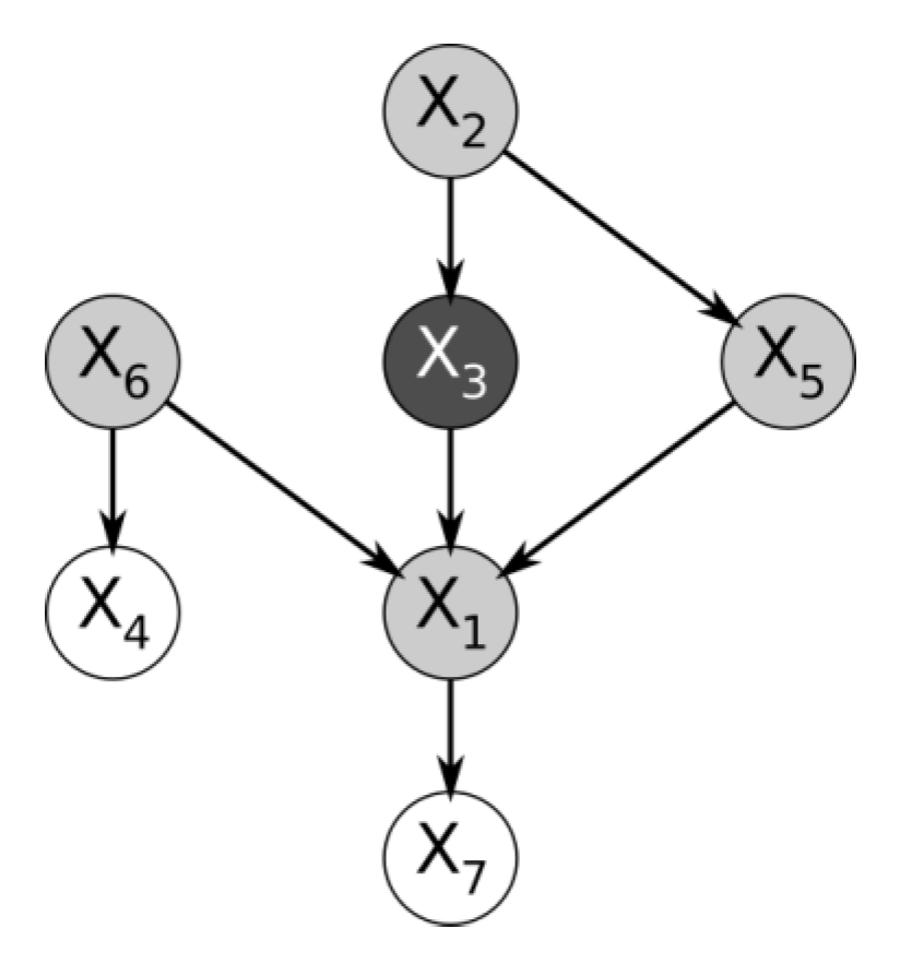
The fact that the edges of a Bayesian network are directed enables it to encode the marginal dependence of a cause and its effect distinctly from the conditional dependence between two causes that share the same effect, given the effect is known, and the causes are otherwise marginally independent. This is the case of the variables $X_1$, $X_3$, $X_5$ and $X_6$ from the simple Bayesian network in Figure 1.

Here, the conditional probability table of variable $X_1$ is only defined based on variables $X_3$, $X_5$ and $X_6$. However, if $X_1$ were not part of the dataset at all, then $X_6$ would appear marginally independent of either $X_5$ and $X_3$. But the Bayesian network correctly expresses the fact that knowing $X_1$ would render $X_6$ dependent on both $X_3$ and $X_5$, because knowing one cause and its effect provides information about the other causes that share the effect.

In the Bayesian network shown in Figure 1, the variables $X_6$, $X_3$ and $X_5$ are the “parents” of $X_1$, which is their “child”. Because they share a child, $X_6$, $X_3$ and $X_5$ are “spouses”.

To correctly determine the true relationship between these variables in the network, the d-separation criterion is applied, as discussed in Section 3.1. This criterion works by giving special meaning to nodes that have converging or diverging arrows. In other words, a path between two nodes cannot be unambiguously interpreted on its own as “dependence” or “independence” (d-connected or d-separated, respectively). The direction of the edges that compose it must be taken into account, along with the conditioning set.

In a Bayesian network, the Markov boundary of a variable $X_i$ is the smallest subset of variables which renders $X_i$ conditionally independent of the entire Bayesian network, given the Markov boundary itself, not only of its ancestors. Therefore, if $\mathit{U}$ is the set of all the variables of the dataset and $MB\left(X_i\right)$ is the Markov boundary of $X_i$, then

$$I(X_i|MB\left(X_i\right)|\mathit{U}-MB\left(X_i\right)-X_i).$$

(2)

Note that the network may contain multiple sets for which this property holds. They are called Markov blankets, and the Markov boundary is the smallest blanket. The Markov boundary is also unique for a specific variable $X_i$ [2].

Due to this property, knowing the variables in the Markov boundary of $X_i$ renders $X_i$ itself obsolete, because the behavior of $X_i$ can be predicted entirely by its Markov boundary. A Markov boundary is illustrated in the same Figure 1.

It is highly desirable to know the Markov boundary of any individual variable of interest in a dataset because it holds such predictive power for the variable. However, knowing enough boundaries allows for the construction of the complete Bayesian network, which is a much more useful source of information.

As a corollary, knowing the entire Bayesian network that underlies a dataset will trivially reveal all the Markov boundaries of the variables within it [2]: the boundary of a target node consists, by definition, of its parents, children and spouses (the nodes that share children with the target node). However, as stated above, the Bayesian network is usually unknown and the sole source of information is the dataset itself.

The Markov boundary and the Markov blanket are concepts originating from Markov networks, which are similar encodings to Bayesian networks, but are undirected graphs, which limits their expressive power [2]. For this reason, Bayesian networks are preferred when encoding causal information. However, there are relationships that Bayesian networks cannot represent but Markov networks can [2].

3.1. The d-Separation Criterion

In order to determine whether two variables of a Bayesian network are independent or not, given a conditioning set of other variables, the directional separation (d-separation) criterion must be applied [2]. By definition, two variables are independent given the conditioning set if all the paths between their corresponding nodes in the network contain either:

• A node with diverging edges, which is in the conditioning set, or
• A node with converging edges, which is outside the conditioning set and also all of its descendants are outside the conditioning set.

If there is a path in the network that connects the two nodes but contains no node for which any of the above conditions is broken, then the two variables are dependent even after the conditioning set is given [2]. In this case, the nodes that represent the variables are said to be d-connected, as opposed to d-separated.

Conversely, a path that contains a node for which the above conditions hold is considered a “blocked” path, thus it will not convey dependence. If all possible paths between two specific nodes are blocked given the conditioning set, then the nodes are d-separated, thus the variables they represent are conditionally independent given the conditioning set.

Because the d-separation criterion simply evaluates to either “dependent” or “independent” when applied to two variables and a conditioning set, it is obvious that Markov Boundary Discovery algorithms can use d-separation just as easily as using a statistical test of independence. As stated earlier, applying the d-separation criterion requires the Bayesian network.

4. Algorithms and Implementation

Two algorithms were chosen for the experiment, namely IAMB and IPC-MB, presented in context in Section 2. Both algorithms have been implemented in an easily configurable form compatible with any kind of CI test. The implementations and the experimental framework are part of the Markov Boundary Toolkit (MBTK) [17], a free and open-source library designed for research on Markov boundary discovery algorithms. MBTK is implemented in Python and contains all the components used by this experiment. This library was also used to implement and evaluate the $dcMI$ optimization [10]. Wherever the G-test is used in the experiment, its computation is accelerated with $dcMI$.

The following two subsections describe the aforementioned algorithms, and a third subsection discusses the implementation of the algorithm for the d-separation criterion used in the experiment.

4.1. IAMB

The Incremental Association Markov Blanket (IAMB) [9] algorithm discovers the Markov boundary of a target variable by running two phases. In the first phase, called the forward phase, the algorithm constructs a set of candidate variables based on their correlation with the target variable. In the second phase, the algorithm eliminates the candidates that are rendered conditionally independent from the target given the other candidates [9].

IAMB relies on conditional mutual information as a heuristic for correlation, used to determine which variables are good candidates for the Markov boundary. The CI test employed by IAMB is thresholded conditional mutual information.

The authors of PCMB [7] have compared their algorithm to IAMB and, interestingly, they mention that IAMB uses the G-test for conditional independence. Moreover, they mention that it uses the p-value of the test as a heuristic for correlation. However, IAMB relies on conditional mutual information, as stated earlier. On the other hand, the G-test is indeed used by HITON [5] and MMMB [6], also discussed in the PCMB article [7]. This minor inconsistency is addressed here because it is present in the references of the current article.

Regardless, IAMB can indeed be adapted to use the G-test due to the relationship of the G-test with the mutual information upon which IAMB originally relied. This replacement was made for the experiment for consistency with IPC-MB and in order to avoid having to choose a manual threshold for conditional mutual information.

Moreover, IAMB can also use d-separation as a CI test with ease, but it still requires a heuristic for correlation. To address its need for a heuristic, a synthetic heuristic was implemented which only relies on the Bayesian network. It returns the following values:

• The length of the shortest path between the corresponding nodes in the Bayesian network, if the two variables of interest are d-connected, given the conditioning set;
• The value 0, if the two variables of interest are d-separated, given the conditioning set.

This replacement was possible because IAMB only uses the heuristic to compare variables among themselves. The data-processing inequality [18] makes the length of the path an acceptable replacement for this specific case.

4.2. IPC-MB

The Iterative Parent–Child-Based Search of Markov Blanket (IPC-MB) [11] algorithm takes a more fine-grained approach and breaks the discovery problem into smaller subproblems. It relies on concepts refined by PCMB [7], originally introduced by HITON [5] and MMMB [6]. In short, IPC-MB first discovers the parents and children of the given target variable, then repeats this discovery process for each of the parents and children. The goal is to find the spouses of the target variable, which are the variables that have common children with the target.

The key improvement of IPC-MB lies in the tactic employed when searching for parents and children: it ensures that the first CI tests performed during the search are those with the smallest conditioning set. The algorithm ensures this by iteratively incrementing the size of the conditioning set used in the CI tests. This way, the algorithm eliminates false positives as early as possible, therefore performing fewer tests. Moreover, the tests that it needs to perform have smaller conditioning sets overall.

IPC-MB requires no heuristic at all, only a CI test implementation. This makes IPC-MB very appropriate for the experiment described in this article.

4.3. d-Separation

Currently, MBTK contains a very simple but inefficient algorithm for computing d-separation. The algorithm is essentially a straightforward implementation of the definition of the d-separation criterion [2,19]. It is very simple because it enumerates all possible undirected paths between two nodes and then checks each node on each path to see if it ‘blocks’ the path, following the conditions described in Section 3.1. However, at the same time, this simplicity is detrimental. Its inefficiency is largely caused by the full enumeration of paths, and the number of paths between two nodes can be exponential in the size of the graph [19]. The algorithm is defined as follows:

Algorithm 1 shows the pseudocode for computing the d-separation criterion as it is currently implemented in MBTK. The procedure DSeparation receives two nodes X and Y as arguments, along with a conditioning set $\mathit{Z}$, and returns true or false indicating whether X and Y are independent or not given the nodes in $\mathit{Z}$. As stated earlier, the MBD algorithms only truly need the binary information about the conditional independence of two variables given a conditioning set, therefore the DSeparation procedure above is sufficient for their operation. The procedure FindAllUndirectedPaths was not specified in detail in Algorithm 1 because it is a generic graph operation.

Algorithm 1 Simple algorithm for computing d-separation

1: procedureDSeparation($X,Y:\mathrm{Node},\mathit{Z}:\mathrm{List}\left[\mathrm{Node}\right]$)  2:     $paths$ = FindAllUndirectedPaths$(X,Y)$  3:     for all $path\in paths$ do  4:      if ¬IsPathBlockedByNodes($path,\mathit{Z}$) then  5:      return FALSE  6:     return TRUE  7:    8: procedure IsPathBlockedByNodes($path,\mathit{Z}:\mathrm{List}\left[\mathrm{Node}\right]$)  9:     for all $node\in path[1:-1]$do           ▹ skip first and last nodes 10:        $isCollider$ = IsNodeCollider$(path,node)$ 11:        $hasConditionedDescendants=\exists n\in node.descendants$ such that $n\in \mathit{Z}$ 12:        if $isCollider\wedge node\notin \mathit{Z}\wedge \neg hasConditionedDescendants$ then 13:        return TRUE 14:        if $\neg isCollider\wedge n\in \mathbf{Z}$ then 15:        return TRUE 16:     return FALSE 17:   18: procedure IsNodeCollider($path:\mathrm{List}\left[\mathrm{Node}\right],node:Node$) 19:     $edgeInboundFromPrev$ = $node\in node.previous.descendants$ 20:     $edgeInboundFromNext$ = $node\in node.next.descendants$ 21:     return $edgeInboundFromPrev\wedge edgeInboundFromNext$ 22:   23: procedure FindAllUndirectedPaths($start,end:\mathrm{Node}$)    ▹ unspecified for brevity

For context, Koller and Friedman [19] present a much more efficient algorithm informally called Reached (the name of the procedure in their pseudocode). The Reached algorithm is linear in the size of the graph, but it is far more complex. Because the Bayesian networks chosen for the experiment are quite small, implementing Reached was deemed unnecessary at the time.

5. Experiment and Results

An experiment was implemented to illustrate the use of the d-separation criterion when evaluating MBD algorithms. A selection of three Bayesian networks were used throughout the experiment. These are the CHILD, ALARM and MILDEW networks, part of the bnlearn repository [20]. The CHILD network consists of 20 nodes, the ALARM network consists of 37 and MILDEW consists of 35. The repository classifies the size of these three networks as “medium networks” [20].

The experiment contains two groups of algorithm runs, called $BN$ and $DS$, based on the source of CI information used by the algorithms when discovering Markov boundaries:

• The $BN$ group contains algorithm runs where the CI information was the d-separation criterion exclusively, computed on the three Bayesian networks in their original, abstract form; the runs in the $BN$ group do not require any sampling or dataset synthesis;
• The $DS$ group contains algorithm runs that apply statistical CI tests on synthetic datasets randomly generated from the three Bayesian networks; the $DS$ group also uses the d-separation criterion on the original Bayesian networks, but only to record the accuracy of each test, where ‘accurate’ means in agreement with the d-separation criterion, while ‘inaccurate’ means in disagreement.

5.1. The Algorithm Runs in the $BN$ Group

The $BN$ group consists of algorithm runs that use d-separation as a CI test exclusively and no dataset was synthetically generated for them. There are 6 algorithm runs in total: each of the 2 algorithms has one run for each of the 3 Bayesian networks.

Of interest are the following measures:

• The total number of CI tests performed by the algorithms on each Bayesian network, considered a measure of the overall efficiency of the algorithms;
• The average size of the conditioning set used in the CI tests, considered a measure for the overall sample efficiency of the algorithms.

Table 1. Overall d-separation test count and average conditioning set size.

Algorithm	Network	Tests	Avgerage Cond. Set Size	Duration (s)
IAMB	CHILD	148	9.66	0.001
IAMB	ALARM	319	11.41	0.005
IAMB	MILDEW	407	13.95	0.104
IPC-MB	CHILD	32,310	5.96	0.360
IPC-MB	ALARM	57,831	4.06	4.793
IPC-MB	MILDEW	313,479	5.60	87.281

confirms what was already reported by the authors of IPC-MB [16], but the information presented in this table is far more accurate due to the exclusive usage of d-separation as a CI test instead of statistical tests. Indeed, IAMB performs far fewer CI tests than IPC-MB, but the tests it performs have much larger conditioning sets, unequivocally revealing that IAMB is sample inefficient. The values indicating the highest efficiency per column are shown bolded.

It is worth emphasizing that these results are fully repeatable and deterministic, depending only on the structure of the Bayesian networks and on the design of the algorithms. There is no randomly synthesized dataset, no sampling process that could be biased and no scarcity of samples for specific combinations of variables. It can be considered that these runs to have been performed in ideal conditions, because the algorithms received perfect information about the CI relationships between variables.

The “Duration” column in Table 1 shows that running MBD algorithms exclusively configured with d-separation consumes very little computing time, even with the simple and very inefficient method described by Algorithm 1. This is essential, because it means that such validation runs can be executed as software integration tests when developing MBD algorithms. The method described by Koller and Friedman [19], mentioned in Section 3.1, would reduce the duration even further.

5.2. The Algorithm Runs in the $DS$ Group

The $DS$ group consists of runs that use the statistical G-test on synthetic datasets to discover the Markov boundaries of variables, but each test is also verified using the d-separation criterion for the tested variables on the source Bayesian network. The d-separation result is recorded for later analysis. A random sampler was employed to generate datasets of 800, 4000, 8000 and 20,000 samples for each of the three Bayesian networks in the experiment.

Of interest are the following measures:

• The total number of CI tests performed by the algorithms on each dataset, considered a measure of the overall efficiency of the algorithms;
• The percentage of statistical tests performed by the algorithms that were accurately evaluated, i.e., the statistical tests in agreement with the simultaneously computed d-separation criterion;
• The average size of the conditioning set used in the CI tests, considered a measure for the overall sample efficiency of the algorithms;
• The precision–recall Euclidean distance from perfect precision and recall, as calculated by the authors of PCMB [7] and of IPC-MB [11].

Table 2. G-test results across all datasets of 800 samples for IAMB and IPC-MB.

Algorithm	Network	Tests	Average Cond. Set Size	Accurate Tests	PR Distance	Duration (s)
IAMB	CHILD	144	10.78	86.11%	0.216	1.070
IAMB	ALARM	223	6.18	89.24%	0.235	0.484
IAMB	MILDEW	713	9.63	20.48%	0.827	5.179
IPC-MB	CHILD	10,581	3.94	92.74%	0.366	22.225
IPC-MB	ALARM	19,042	2.34	92.70%	0.270	30.213
IPC-MB	MILDEW	4176	1.34	42.94%	1.306	8.240

,

Table 3. G-test results across all datasets of 4000 samples for IAMB and IPC-MB.

Algorithm	Network	Tests	Average Cond. Set Size	Accurate Tests	PR Distance	Duration (s)
IAMB	CHILD	177	18.42	77.97%	0.097	9.783
IAMB	ALARM	255	8.25	93.73%	0.165	2.098
IAMB	MILDEW	1019	22.55	28.95%	0.711	83.683
IPC-MB	CHILD	26,588	6.67	97.65%	0.022	237.000
IPC-MB	ALARM	26,430	2.72	94.62%	0.116	131.340
IPC-MB	MILDEW	10,104	1.46	59.12%	1.122	70.179

,

Table 4. G-test results across all datasets of 8000 samples for IAMB and IPC-MB.

Algorithm	Network	Tests	Average Cond. Set Size	Accurate Tests	PR Distance	Duration (s)
IAMB	CHILD	207	23.44	67.63%	0.137	27.523
IAMB	ALARM	267	9.01	95.51%	0.144	4.248
IAMB	MILDEW	1131	24.17	30.15%	0.668	193.901
IPC-MB	CHILD	25,343	6.64	97.89%	0.039	357.632
IPC-MB	ALARM	33,183	2.94	94.84%	0.115	310.035
IPC-MB	MILDEW	18,536	1.64	69.50%	0.880	229.154

and

Table 5. G-test results across all datasets of 20,000 samples for IAMB and IPC-MB.

Algorithm	Network	Tests	Average Cond. Set Size	Accurate Tests	PR Distance	Duration (s)
IAMB	CHILD	178	22.79	75.28%	0.079	57.649
IAMB	ALARM	277	9.24	96.75%	0.109	10.230
IAMB	MILDEW	1220	28.49	28.11%	0.702	611.964
IPC-MB	CHILD	37,240	6.88	98.85%	0.000	1177.597
IPC-MB	ALARM	36,139	2.95	95.34%	0.121	792.971
IPC-MB	MILDEW	33,480	2.45	85.62%	0.467	978.469

capture the behavior of IAMB and IPC-MB with G-tests on the three Bayesian networks, recording the measures of interest mentioned above. There are a few interesting facts to observe in the results. Values representing the highest efficiency and accuracy in their respective columns are shown bolded.

Firstly, IPC-MB has issues with the MILDEW datasets of 800, 4000 and 8000 samples, resulting in high PR distances, while IAMB performs much better. This happens in spite of IPC-MB performing tests with very small conditioning sets. This is also not an effect of inaccurate tests, because the d-separation results agree with the G-tests performed by IPC-MB almost twice as often as for IAMB. Still, IAMB produces much more accurate Markov boundaries (lower PR distances) in spite of performing G-tests that end up being accurate in less than $30\%$ of cases, for any dataset size. A simple and satisfactory explanation for this observation could not be found as part of this experiment, although it was indeed surprising. At this moment, an implementation mistake cannot be ruled out, although this is highly unlikely because IAMB and IPC-MB have been developed under the same suite of unit tests and they also produce the same Markov boundaries when configured with the d-separation CI test. It is also worth mentioning that MILDEW causes the lowest CI test accuracies of all the Bayesian networks for both algorithms at all sample sizes. On top of that, IAMB appears to be more accurate than IPC-MB for all datasets of 800 samples.

Apart from the anomaly described above, IPC-MB consistently outperforms IAMB with respect to accuracy, producing lower PR distances. On the CHILD dataset at 20,000 samples, IPC-MB achieves $0.000$ PR distance, the best value in the experiment.

Secondly, the average conditioning set size in the G-tests performed by the algorithms grows as the number of samples in the dataset grows. The most noteworthy increase is observed for IAMB on the MILDEW dataset: at 800 samples, IAMB performs tests with an average conditioning set size of $9.63$, but at 20,000 samples, this average becomes $28.49$. Note that the entire MILDEW network consists of 35 nodes in total and $28.49$ represents $81.4\%$ of the whole network.

In contrast, IPC-MB appears much more stable: the greatest difference in the average conditioning set size is seen on the CHILD datasets, but it starts at $3.94$ at 800 samples and reaches $6.88$ at 20,000 samples, a much smaller increase than that which is observed for IAMB.

Thirdly, the d-separation validations recorded for the G-tests reveal another interesting fact: the CI tests performed by IAMB do not have a clear trend in accuracy with respect to sample size, but those performed by IPC-MB become more and more accurate as sample size increases. The lack of a trend in IAMB is somewhat surprising, because a higher sample count should provide more accurate tests, but this potential increase in accuracy is cancelled by the growing average conditioning set seen for IAMB as the sample count increases, described above.

The values in the “Duration” column in Table 2, Table 3, Table 4 and Table 5 reinforce the fact that CI tests consume the overwhelming majority of the computing resources used by an MBD algorithm. It also highlights another drawback of CI tests when used during algorithm development, namely the delay they introduce in the design loop. However, the G-test was computed here with the $dcMI$ optimization, which can reduce the computation time of the G statistic by a factor of 20 [10]. Without optimization, the durations observed in this experiment would have been much greater.

However, configuring an MBD algorithm to use a statistical CI test alongside d-separation during the design phase may be a necessary condition, depending on the algorithm, as hypothesized in the Introduction (Section 1).

6. Conclusions

The main contribution of this article is the proposed usage of d-separation when designing, developing and evaluating Markov Boundary Discovery algorithms. Thus, it discussed how the d-separation criterion can help researchers design and validate novel MBD algorithms. This usefulness stems from it being a perfect source of conditional independence information, unlike statistical tests, and it is far more efficient to compute than a statistical test, shortening the design feedback loop considerably.

Moreover, adding the d-separation criterion as a CI test to Markov boundary discovery algorithms has the potential to provide researchers and algorithm designers with new and unexpected insights into the behavior of the algorithms. Of course, computing d-separation requires the Bayesian network to be known, but this is normally the case when evaluating algorithms on synthetic data. In the exemplifying experiment presented in this article, a new measure was described consisting of the percentage of accurate statistical tests. This measure would not have been possible without implementing d-separation itself as a CI test. The observed behavior of algorithms also presented an unexpected anomaly which needs to be studied and explained in a future analysis. However, this is only a simple attempt to illustrate the possibilities that open up when d-separation is an integral part of the experiment.