Article

Multi-Fidelity Sparse Polynomial Chaos and Kriging Surrogate Models Applied to Analytical Benchmark Problems

1
Department of Mechanical and Aerospace Engineering, University of Dayton, Dayton, OH 45469, USA
2
Air Force Research Laboratory, Wright-Patterson Air Force Base, OH 45433, USA
*
Author to whom correspondence should be addressed.
Algorithms 2022, 15(3), 101; https://doi.org/10.3390/a15030101
Submission received: 7 February 2022 / Revised: 17 March 2022 / Accepted: 18 March 2022 / Published: 21 March 2022

Abstract

:
In this article, multi-fidelity kriging and sparse polynomial chaos expansion (SPCE) surrogate models are constructed. In addition, a novel combination of the two surrogate approaches into a multi-fidelity SPCE-Kriging model will be presented. Accurate surrogate models, once obtained, can be employed for evaluating a large number of designs for uncertainty quantification, optimization, or design space exploration. Analytical benchmark problems are used to show that accurate multi-fidelity surrogate models can be obtained at lower computational cost than high-fidelity models. The benchmarks include non-polynomial and polynomial functions of various input dimensions, lower dimensional heterogeneous non-polynomial functions, as well as a coupled spring-mass-system. Overall, multi-fidelity models are more accurate than high-fidelity ones for the same cost, especially when only a few high-fidelity training points are employed. Full-order PCEs tend to be a factor of two or so worse than SPCES in terms of overall accuracy. The combination of the two approaches into the SPCE-Kriging model leads to a more accurate and flexible method overall.

1. Introduction

The North Atlantic Treaty Organization (NATO) Science and Technology Organization (STO) working group AVT-331 “Goal-driven, multi-fidelity approaches for military vehicle system-level design” is currently investigating computing frameworks that could significantly impact the design of next-generation military vehicles [1]. In order to save computational time for uncertainty quantification, optimization, or design space exploration, the use of surrogate models can be a very good strategy. In a surrogate model, expensive function evaluations are replaced by an approximation, which is computationally inexpensive and can thus be evaluated extensively. Especially polynomial chaos expansions (PCEs) [2,3,4] and kriging [5,6,7,8] have been widely used in the community. Kriging accuracy can be improved by a dynamic training point selection process rather than picking all training points randomly at the beginning [9]. This is analogous to the concept of expected improvement (EI) which tries to keep a balance between exploration (space filling) and exploitation (resolve interesting areas in the design space).
PCE [10,11,12,13] and kriging [14,15,16,17,18] models support the usage of both high- and lower fidelity training points. A standard multi-fidelity strategy is to combine fittings of the high-fidelity (HF) data (e.g., better models, experimental data, finer meshes) with trends from cheaper, low-fidelity (LF) data (e.g., less sophisticated models, coarser meshes). Thus, the usually less intensively sampled HF data needs to correct the trends given by the intensively sampled LF data, for instance, via the popular correction-based method [18]. The correction function is known as scaling function, calibration, or bridge function, and can be additive [19,20], multiplicative [21], or hybrid multiplicative/additive [10,11,13].
Additionally, the compressive sensing (CS) theory [22,23,24,25,26,27,28,29] has shown great potential to reduce the curse of dimensionality for PCEs depending on the decay rate of the PCE coefficients and thus the underlying sparsity of the solution. CS offers a framework to use fewer training points than basis functions and to still recover a good approximation to the sparse solution [27,28,29,30]. CS also increases the robustness to noise thanks to the introduced sparsity constraint [28,29]. In summary, CS aims at selecting a small number of basis polynomials with great impact on the model response [31] and the resulting surrogate model is called sparse PCE (SPCE).
Thus far, these two distinct surrogate modeling approaches (SPCE and kriging) have been applied in various fields more or less standalone. There have been a few attempts to combine kriging and SPCE in a systematic way for single-fidelity applications [32,33], but none for multi-fidelity. SPCE is well known for capturing the overall trends of the solution, whereas kriging handles the values around training points well [32,33]. In this work, a proposed MF SPCE-Kriging method aims at combining the advantages of both meta-modeling methods, thus expecting fewer training points to be required for constructing an accurate model in lieu of computationally expensive HF simulations.
The general goal of this work is to construct very accurate surrogate models at small overall computational cost assuming that the dominant cost factor is obtaining high-fidelity training point information. The strategy to accomplish this is to enhance surrogate modeling techniques by employing lower fidelity information, adaptively selecting training points, as well as compressed sensing and to use a combined SPCE-Kriging meta-modeling method.

2. Methodology

The multi-fidelity kriging and sparse PCE methods in Section 2.2 and Section 2.3 have been presented in previous works [30,34,35], but are briefly presented here for completeness. Section 2.4 presents the novel combination of the two methods, but first a brief overview of universal kriging is given in Section 2.1.

2.1. Single-Fidelity Universal Kriging

Kriging [5] is a Gaussian random process realization to estimate a function value in a sample location, f ^ ( x ) :
f ^ ( x ) = β T h ( x ) + Z ( x )
where β T h ( x ) is the mean value or trend of the Gaussian process and Z ( x ) represents a stationary Gaussian process with zero mean, variance σ 2 and the covariance of two locations, x i and x j , is given by C o v Z ( x i ) , Z ( x j ) = σ 2 R ( x i , x j , θ ) where R is an auto-correlation function, which is only dependent on the distance between the two locations due to stationarity and a hyper-parameter, θ . In this work Wendland C4 [36] auto-correlation functions are employed. The most general kriging formulation is called universal kriging, in which the mean is given by a sum of P + 1 pre-selected trend functions, h k ( x ) , that is
β T h ( x ) = k = 0 P β k h k ( x )
where β k are the trend coefficients. In ordinary kriging the mean has a constant but unknown value, so P = 0 , h 0 ( x ) = 1 , and β 0 is unknown.
Given a value for θ the calibration of the universal kriging model parameters can be computed analytically using an empirical best linear unbiased estimator (BLUE):
β ( θ ) = H T R 1 H 1 H R 1 Y
σ 2 ( θ ) = 1 N Y H β T R 1 Y H β
where Y = f ( x i ) , i = 1 , , N are the N training point observations and H i j = h j ( x i ) is the information matrix.
The optimal θ ^ is determined here by maximization of a log-likelihood function via a genetic algorithm (for more details see Yamazaki et al. [16]):
θ ^ = a r g m a x θ N ln ( σ 2 ) ln ( d e t ( R ) )
and the resulting β ( θ ^ ) can then be used to predict the kriging response via
f ^ ( x ) = β T h ( x ) + r ( x ) T R 1 Y H β
where r i ( x ) = R ( x , x i , θ ^ ) is the correlation between a new sample location, x, and an existing training point, x i .

2.2. Multi-Fidelity Kriging

In order to create a multi-fidelity surrogate model one has to map the trend of the more intensively sampled low-fidelity (LF) data to the less intensively sampled high-fidelity (HF) data. Here, a hybrid bridge function approach adopted from Han et al. [18] is used that has been presented in previous work [37]. The relationship between low- and high-fidelity surrogate model values (indicated by a hat) in any location x is given by
f ^ H F ( x ) = ϕ ^ ( x ) f ^ L F ( x ) + γ ^ ( x )
where ϕ ^ ( x ) = g T ( x ) ρ ^ is a low-order polynomial with q + 1 basis functions g T ( x ) = [ 1 , g 1 ( x ) , , g q ( x ) ] and corresponding coefficients ρ ^ = [ ρ ^ 0 , ρ ^ 1 , , ρ ^ q ] T and γ ^ ( x ) is an additive bridge function. A multi-fidelity kriging surrogate model is constructed via the following three steps (visualized in Figure 1):
1.
Using N L F 1 lowest fidelity training points construct a kriging model, f ^ L F 1 .
2.
Construct another kriging model for the additive bridge function, γ ^ 2 , where γ 2 ( x i ) = f L F 2 ( x i ) ϕ ^ 2 ( x i ) f ^ L F 1 ( x i ) in N L F 2 training points. Compute an optimal ρ ^ 2 (and θ ^ 2 ) during the maximum likelihood estimation updates for γ ^ 2 , which means training point values γ 2 ( x i ) will change constantly, but once converged one can evaluate f ^ L F 2 ( x ) = ϕ ^ 2 ( x ) f ^ L F 1 ( x ) + γ ^ 2 ( x ) .
3.
Repeat step 2 until reaching the highest fidelity level (this is analogous to a multi-grid strategy).
Numerical experimentation showed what intuition suggests namely that the HF training locations should be a subset of the LF locations to make sure that no error is added from f ^ L F ( x ) when computing γ ( x ) = f H F ( x ) ϕ ^ ( x ) f ^ L F ( x ) in all N H F training points. The other ( N L F N H F ) LF training locations are selected via latin hypercube sampling subject to a distance constraint to the existing HF points. Furthermore, whenever the dynamic training point algorithm [9] adds a HF point to the set, the corresponding LF point is also added.

2.3. Multi-Fidelity Sparse Polynomial Chaos Expansions

An all-at-once approach developed by Bryson and Rumpfkeil [13] is used to simultaneously determine additive, x , and multiplicative, x , corrections to the low-fidelity data to best approximate the high-fidelity function in a least-squares sense:
f ^ H F ( x ) = f ^ L F ( x ) + α ( x ) f ^ L F ( x ) + δ ( x ) .
A non-intrusive point collocation regression procedure is employed and the PCE coefficients are determined by a singular value decomposition. Gauss–Patterson knots are used to determine the training points and higher grid levels contain the lower levels as a subset. In particular, Smolyak sparse grids with a slow-exponential growth rule are used via Burkardt’s sparse grid mixed growth anisotropic rules library [38].
For the compressive sensing one can recover the signal b ^ from an incomplete measurement vector Y by solving an optimization problem of the form
min b ^ 0.5 | | A b ^ Y | | 2 2 + λ | | b ^ | | 1
where λ is a penalty coefficient and A is the regression matrix. The LASSO (least absolute shrinkage and selection operator) algorithm is employed to solve Equation (9) implemented via the software library mlpack [39]. Note that selecting a good value for λ is crucial: If λ is too small, it may result in over-fitting or a less sparse solution, while for large values of λ , the reconstructed signal may not be accurate enough. Following Salehi et al. [31] to determine an optimal λ ^ , either the leave-one-out cross-validation error [40] or a true root-mean-square error (RMSE) has been used in previous work [30] and the latter is employed here. In order to find λ ^ , the optimization problem is solved for various values of λ and the corresponding RMSE is computed. Then, λ ^ is defined as the value of λ yielding the smallest RMSE.

2.4. Multi-Fidelity SPCE-Kriging

The descriptions given in Section 2.1 and Section 2.3 show that kriging is interpolatory in nature and PCE is a regression. Thus, kriging usually recreates the local variations well, whereas PCE captures the global trends better [32,33]. Therefore, it is natural to try to combine the advantages of both kriging and SPCE for a more efficient meta-modeling technique. The resulting SPCE-Kriging model is a kriging surrogate, whose trend functions are determined by an SPCE model using the same underlying training data. The construction of a single-fidelity SPCE-Kriging consists of the following three main steps:
1.
Choose PCE orthogonal bases associated with the probability distributions of the (random) inputs;
2.
Solve for the PCE coefficients using the LASSO algorithm as described in Section 2.3 to determine which bases are most important;
3.
Use only those important bases as trend functions h k in the universal kriging mean value given by Equation (2) as well as in the maximum likelihood estimation using Equation (5).
For the construction of a multi-fidelity SPCE-Kriging, which to the authors’ knowledge is a novel contribution, the algorithm presented in Section 2.2 is employed. However, there is an important caveat: SPCE-Kriging is only used in the first step (the training of the lowest fidelity surrogate model, f ^ L F 1 ) and for the additive bridge function, γ ^ 2 , an ordinary kriging model is constructed. The reason for this is that in step two, the genetic algorithm requires a lot of log-likelihood evaluations to compute the optimal ρ ^ 2 (and θ ^ 2 ), which is required to compute ϕ ^ 2 ( x ) = g T ( x ) ρ ^ 2 and thus the N L F 2 training points for the additive bridge function, γ 2 ( x i ) = f L F 2 ( x i ) ϕ ^ 2 ( x i ) f ^ L F 1 ( x i ) . Hence, using SPCE-Kriging for the construction of the additive bridge function, γ ^ 2 , would require a lot of SPCE evaluations, which are much more expensive than simple ordinary kriging constant trend computations.

3. Numerical Experiments Setup

The AVT-331 group aims to investigate goal-driven, multi-fidelity approaches for the system-level design of military vehicles, which usually requires the solution of optimization problems and the exploration/visualization of the global design space.

3.1. Assessment Metric

In order to assess the global accuracy of a surrogate model the root mean square error (RMSE) between the exact, f, and surrogate function predictions, f ^ , calculated on a D-dimensional Cartesian mesh with N t total nodes will be used
RMSE = 1 N t i = 1 N t f i f ^ i 2 .
If the surrogate model is not deterministic (e.g., kriging) it will be executed five times, and the average RMSE and its standard deviation will be reported. For a deterministic surrogate (e.g., PCE) a single run is sufficient. The Cartesian mesh is equispaced with N x nodes in one coordinate direction as given in Table 1.
Note that for D = 10 not the entire normalized interval [ 0 , 1 ] is covered but rather only [ 0.05 , 0.95 ] since otherwise a majority of the points are likely located in the extrapolation regimes of the surrogate models, which tend to be less accurate.

3.2. Benchmark Problems

Table 2 summarizes the recommended analytical benchmarks by the AVT-331 group to assess and compare the performance of multifidelity methods. The following subsections provide more details for each of the functions.

3.2.1. Forrester Function

The Forrester function [41] is a well-known one-dimensional benchmark for multi-fidelity methods, described by the following equations in the domain 0 x 1 (from 1 highest fidelity to 4 lowest fidelity level) and shown in Figure 2.
f 1 ( x ) = 6 x 2 2 sin ( 12 x 4 )
f 2 ( x ) = 5.5 x 2.5 2 sin ( 12 x 4 )
f 3 ( x ) = 0.75 f 1 ( x ) + 5 ( x 0.5 ) 2
f 4 ( x ) = 0.5 f 1 ( x ) + 10 ( x 0.5 ) 5

3.2.2. Rosenbrock Function

The Rosenbrock function is a well-known D-dimensional optimization benchmark problem in [ 2 , 2 ] D described by the following equation:
f 1 ( x ) = i = 1 D 1 100 x i + 1 x i 2 2 + 1 x i 2
The global minimum is inside a long, narrow, parabolic shaped flat valley. It is relatively straightforward to capture the overall quartic shape, but it is difficult to capture the local flat valleys.
The extension to multi-fidelity is described by the following equations, where f 2 can be considered as a medium-fidelity level and f 3 as the lowest fidelity.
f 2 ( x ) = i = 1 D 1 50 x i + 1 x i 2 2 + 2 x i 2 i = 1 D 0.5 x i
f 3 ( x ) = f 1 ( x ) 4 i = 1 D 0.5 x i 10 + i = 1 D 0.25 x i
The three-fidelity levels are shown for two dimensions in Figure 3.

3.2.3. Shifted-Rotated Rastrigin Function

To address real-world optimization problems, where the design space of the objective function is usually multi-modal, the Rastrigin function is selected as benchmark. The variable range is defined as x [ 0.1 , 0.2 ] D , and the function is shifted to change the position of the minimum and rotated to change the properties of the function itself within the variable space:
f 1 ( z ) = i = 1 D z i 2 + 1 cos ( 10 π z i )
with
z = R ( θ ) ( x x ) with R ( θ ) = cos θ sin θ sin θ cos θ
where R is the rotation matrix in two dimensions which can be extended to D dimensions by using the Aguilera–Perez algorithm [42] and the rotation angle is set to θ = 0.2 .
The fidelity levels can be defined following the work of Wang and Jin [43] as
f i ( z , ϕ i ) = f 1 ( z ) + e r ( z , ϕ i ) for i = 1 , 2 , 3
with ϕ 1 = 10 , 000 (high-fidelity), ϕ 2 = 5000 (medium-fidelity), and ϕ 3 = 2500 (low-fidelity). The resolution error is given by
e r ( z , ϕ ) = i = 1 D a ( ϕ ) cos 2 ( w ( ϕ ) z i + b ( ϕ ) + π )
with a ( ϕ ) = Θ ( ϕ ) , w ( ϕ ) = 10 π Θ ( ϕ ) , b ( ϕ ) = 0.5 π Θ ( ϕ ) , and Θ ( ϕ ) = 1 0.0001 ϕ . These fidelity levels are displayed in Figure 4.

3.2.4. ALOS Function

This function employs heterogeneous non-polynomial analytic functions defined on unit cubes in one, two, and three dimensions. The one- and two-dimensional high-fidelity functions are taken from Clark and Bae [44] and are given by
f ( x ) = sin [ 30 ( x 0.9 ) 4 ] cos [ 2 ( x 0.9 ) ] + ( x 0.9 ) / 2
and
g ( x , y ) = sin [ 21 ( x 0.9 ) 4 ] cos [ 2 ( x 0.9 ) ] + ( x 0.7 ) / 2 + 2 y 2 sin [ x y ]
An extension to three dimensions is given by
h ( x , y , z ) = sin [ 21 ( x 0.9 ) 4 ] cos [ 2 ( x 0.9 ) ] + ( x 0.7 ) / 2 + 2 y 2 sin [ x y ] + 3 z 3 sin [ x y z ]
Low-fidelity versions are obtained by using linear additive and multiplicative bridge functions:
f L F ( x ) = ( f 1.0 + x ) / ( 1.0 + 0.25 x )
g L F ( x , y ) = ( g 2.0 + x + y ) / ( 5.0 + 0.25 x + 0.5 y )
h L F ( x , y , z ) = ( h 2.0 + x + y + z ) / ( 5.0 + 0.25 x + 0.5 y 0.75 z )
The advantages of this problem are that it is heterogeneous and non-polynomial. The disadvantages are that it cannot be scaled to arbitrary dimensions and that the LF model is a simple non-linear polynomial scaling.
The one- and two-dimensional functions are displayed together with their low-fidelity approximations in Figure 5.

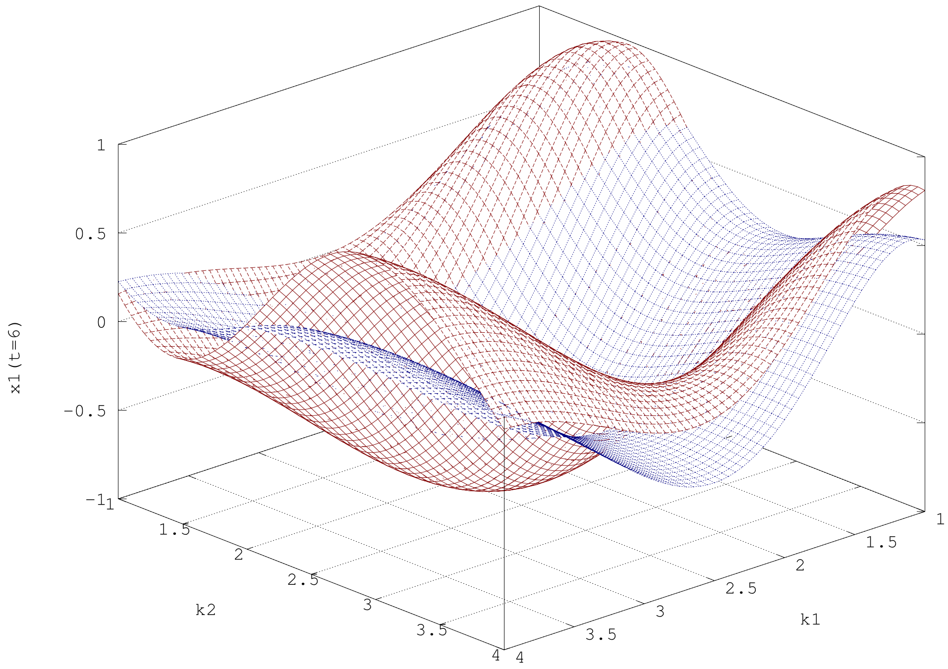
3.2.5. Coupled Spring-Mass-System

Three masses sliding along a frictionless surface are attached to each other by four springs, as shown in Figure 6.
The following constants, variables and assumptions are going to be used in the analysis:
Spring ConstantsThe springs obey Hooke’s law with constants k i ,   i = 1 , , 4 and the mass of each spring is negligible.
Fixed EndsThe first and last spring are attached to fixed walls and have the same spring constant.
Mass Constants m 1 , m 2 , m 3 are point masses.
Position VariablesThe variables x 1 ( t ) , x 2 ( t ) , x 3 ( t ) represent the mass positions measured from their equilibrium positions (negative is left and positive is right).
The equations of motion for this setup are given by
m 1 x ¨ 1 ( t ) = k 1 x 1 ( t ) + k 2 [ x 2 ( t ) x 1 ( t ) ] m 2 x ¨ 2 ( t ) = k 2 [ x 2 ( t ) x 1 ( t ) ] + k 3 [ x 3 ( t ) x 2 ( t ) ] m 3 x ¨ 3 ( t ) = k 3 [ x 3 ( t ) x 2 ( t ) ] k 4 x 3 ( t )
which can be rewritten as
M x ¨ ( t ) = K x ( t )
where the mass matrix M, stiffness matrix K and the displacement x are defined as
M = m 1 0 0 0 m 2 0 0 0 m 3 K = k 1 k 2 k 2 0 k 2 k 2 k 3 k 3 0 k 3 k 3 k 4 x = x 1 x 2 x 3
This is a constant-coefficient homogeneous system of second-order ODEs, the solution of which is given by
x ( t ) = i = 1 3 [ a i cos ( ω i t ) + b i sin ( ω i t ) ] v i
where ω i = λ i and λ i are the eigenvalues of the matrix M 1 K and v i are the corresponding eigenvectors. The constants a i and b i are determined by the initial conditions x ( t = 0 ) = x 0 and x ˙ ( t = 0 ) = x ˙ 0 .

Proposed Benchmark Problem

As a small numerical example, let m 1 = m 2 = 1 , k 1 = k 2 = k 3 = 1 as well as x 0 = ( 1 0 ) T and x ˙ 0 = ( 0 0 ) T , then
M 1 K = 2 1 1 2
with real eigenvalues λ 1 = 1 and λ 2 = 3 and corresponding eigenvectors
v 1 = 1 1 v 2 = 1 1
Since the initial velocity is zero, we have b 1 = b 2 = 0 and using x ( t = 0 ) = x 0 in Equation (30) yields a 1 = a 2 = 0.5 such that
x 1 ( t ) = 0.5 cos ( t ) + 0.5 cos ( 3 t ) and x 2 ( t ) = 0.5 cos ( t ) 0.5 cos ( 3 t )
These solutions are plotted in Figure 7 for 0 t 30 .
Converting Equation (29) into a system of first-order ODEs and using the fourth-order accurate Runge–Kutta time-marching method yields a multi-fidelity analysis problem by varying the time-step size Δ t as shown in Figure 8. Note that the high-fidelity (HF) analysis with Δ t = 0.01 is not distinguishable from the analytical solution given by Equation (31) and shown in Figure 7, while the low-fidelity (LF) analysis with Δ t = 0.6 is exhibiting the correct trends but is somewhat inaccurate.
Treating two spring constants as independent input variables with 1 k 1 = k 3 , k 2 4 while m 1 = m 2 = 1 and computing x 1 ( t = 6 ) yields the two-dimensional design space shown in Figure 9. One can infer that the lower fidelity trends match the high-fidelity ones.
In this work, a two-dimensional (by varying the two spring constants) and four-dimensional (varying two springs and two masses) version of this benchmark problem will be employed. However, other benchmark problems based on this problem for uncertainty quantification and optimization can be easily conceived [35].

4. Results

In the following, the results for each benchmark problem will be shown and discussed. Note that lines are plotted between markers as a visual aide, but do not necessarily reflect performance at intermediate points. For the PCE models, an oversampling ratio of two is always imposed, and the (full-order) PCE results are shown with dashed lines. In general, sparse PCEs (solid lines) outperform full-order PCEs up to a point when the λ term in Equation (9) introduces errors into the fit and the RMSE cannot drop further. SPCE runs for higher than four dimensions (and two for MF) were not possible due to memory issues because of the resulting large matrices. Ordinary kriging results are shown in dashed lines and SPCE-Kriging results (abbreviated as SK in the figures) are displayed in solid lines.
Results for high-fidelity (HF) training data alone are always shown in black whereas multi-fidelity results using fidelity levels 2, 3 or 4 are shown in red, green, and blue, respectively. For the stochastic kriging model, five runs were performed, and the figures show the average RMSE and its standard deviation. The total computational cost is calculated by the sum over all fidelity levels of the product of the number of function evaluations at that level and the given cost at that fidelity level (as given in Table 2). Please note that the vertical error axes differ in each figure since they were chosen to best display each particular result.

4.1. Forrester

The Forrester function results are shown in Figure 10 for both MF SPCE and MF kriging. The acronyms in this and following figures should be interpreted as follows: HF is using high-fidelity data alone with either PCE or ordinary kriging surrogate models whereas HFS and HFSK are employing SPCE and SPCE-Kriging surrogates, respectively. MF2 implies a multi-fidelity surrogate (either PCE or kriging) using data from the highest fidelity level and in this case fidelity level 2. Again, MF2S and MF2SK are instead employing SPCE and SPCE-Kriging surrogates, respectively. Since for MF kriging the number of low-fidelity points can be arbitrary, the starting amount is given. In this case, as 30 LF (that is all the starting HF locations plus latin hypercube sampled locations subject to a distance constraint). The number of LF training points for the MF PCEs is thirty levels higher for the Forrester function (i.e., 63 LF points are used when using 15 HF points). For the MF SPCE models, various orders for the polynomials were combined with several values of λ to find the combination with the lowest root-mean-square error (RMSE). The resulting best values for HF only and MF3 are shown in Table 3. Values for MF2 and MF4 are somewhat similar and are thus omitted here. One can infer that SPCE performs better than PCE up to a point and that MF models perform better than HF models, except for MF2, where the LF model is just too expensive. Kriging performs similarly to PCE when using only a few training points but then falls behind. SPCE-Kriging performs similarly to ordinary kriging.

4.2. Rosenbrock

The Rosenbrock function results are shown in Figure 11 for MF SPCE and in Figure 12 for MF Kriging. The PCE model should match the truth function exactly as soon as sufficient training data is available to build a fourth-order polynomial (including an oversampling ratio of two). For example, the full-order PCE surrogate model requires 30 HF training points in two dimensions and 2002 points in ten dimensions. Some of these points may be LF for the MF models. The number of LF training points in two dimensions is four grid levels higher (i.e., 97 LF points are used when using 17 HF points) and in five and ten dimensions it is one level higher (e.g., 51 HF are combined with 151 LF points in five dimensions and 201 HF are combined with 1201 LF points for ten dimensions). For ten dimensions, a two level difference was also tried, leading to, as expected, a better performance for the cheaper low-fidelity model, but a worse performance for the more expensive one. Overall, the results are behaving as one would expect, verifying that the PCE surrogate models are correctly implemented.
Kriging clearly does not perform as well as PCE for this polynomial test case, but one can infer that MF Kriging at least for the cheaper low-fidelity model outperforms kriging based on HF data alone. One can also see again that an expensive LF model (MF2) is not worth considering. HF SPCE-Kriging performs better than both PCE and SPCE, and MF SPCE-Kriging performs better than MF ordinary kriging, but not as well as HF SPCE-Kriging, though MF3 is better when using only a few HF training points. This demonstrates that the ordinary kriging performance, at least for polynomial functions, can be dramatically improved and also that only using ordinary kriging for the additive bridge function needs to be improved.

4.3. Rastrigin

The Rastrigin function results are shown in Figure 13 for MF SPCE and in Figure 14 for MF Kriging. Again, many different orders for the polynomials were combined with various values of λ to find the combination with the lowest root-mean-square error (RMSE) for the SPCE models. The resulting best values for HF and MF2 for the two-dimensional case are shown in Table 4.
One can infer that SPCE performs better than PCE and that MF models perform better than HF models in the beginning when only a few HF training points are used. Once again, for ten dimensions, a one and two grid level difference was used, leading to, counter-intuitively, a better performance for the more expensive low-fidelity model, but a worse one for the cheaper one. Kriging performs similarly to PCE in both five and ten dimensions, but falls behind for more training points in one dimension. Both HF and MF SPCE-Kriging again perform similarly to ordinary kriging.

4.4. ALOS

The ALOS function results are shown in Figure 15 for MF SPCE and in Figure 16 for MF Kriging. Again, many different orders for the polynomials were combined with various values of λ to find the combination with the lowest root-mean-square error (RMSE) for the SPCE models. The resulting best values for HF and MF2 for the two-dimensional case are shown in Table 5.
As usual, SPCE performs better than PCE up to a point and MF models perform better than HF models in the beginning when only a few HF training points are used. Overall, the performance of the multi-fidelity kriging is somewhat better than MF SPCE in two and three dimensions and somewhat comparable in one dimension. Both HF and MF SPCE-Kriging perform slightly better than ordinary kriging especially when more training points are used and in two and three dimensions.

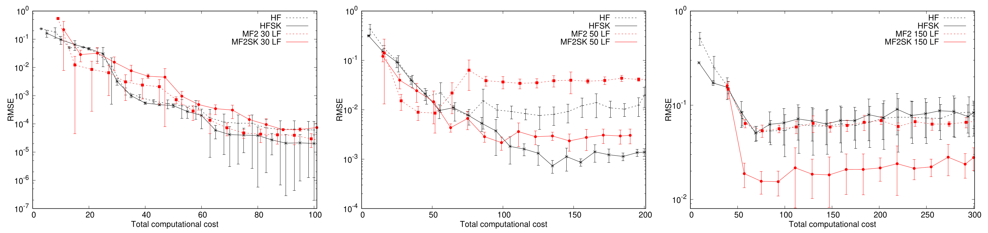
4.5. Coupled Spring-Mass-System

For the MF SPCE models of the coupled spring-mass-system, many different orders for the polynomials were combined with several values of λ to find the combination with the lowest root-mean-square error (RMSE). The resulting best values for the two-dimensional case are shown in Table 6.
The results for these settings are plotted on the left in Figure 17, whereas the performance of a MF kriging model is shown on the right. In general, one can see that the SPCE surrogate models outperform the full order ones (compare solid to dashed lines) again up to a point, and the mono-fidelity models are inferior to the multi-fidelity ones (compare black to red lines) for both the MF SPCE and MF kriging models. Overall, the performance of the multi-fidelity ordinary kriging is comparable to the one of MF SPCE and MF SPCE-Kriging.
In addition to the two-dimensional case, a four-dimensional one where both spring constants and both masses are varied between one and four was considered as well. Again, many different orders for the SPCE are combined with various values for λ to find the combination with the lowest RMSE. The resulting best values are given in Table 7, and the results are shown in Figure 18.
Once again, one can see that the SPCE surrogate model outperforms the full order one (compare solid to dashed line), and the MF models are better than the mono-fidelity ones (compare red to black lines) for both the MF SPCE and MF kriging models. Overall, the performance of the multi-fidelity ordinary kriging is somewhat better than MF SPCE.

5. Conclusions

The goal of this work was to build very accurate surrogate models for applications in design space exploration and optimization, as well as uncertainty quantification at small overall computational cost assuming that the dominant cost factor is obtaining high-fidelity training point information. The employed strategy was to enhance surrogate modeling techniques by employing lower fidelity information and adaptively selecting training points as well as to use compressed sensing and a combined SPCE-Kriging meta-modeling method.
Several analytical benchmark problems have been used to assess the performance of a multi-fidelity sparse polynomial chaos expansion (MF SPCE) model, a MF ordinary kriging model as well as a MF SPCE-Kriging model. Overall, multi-fidelity models are more accurate than high-fidelity ones for the same computational cost especially when only a few high-fidelity training points are employed. Full-order PCEs tend to be a factor of two or so worse than SPCES in terms of overall accuracy as measured by the root-mean-square error (RMSE) compared to a truth model. The combination of the sparse PCE and kriging models into a SPCE-Kriging model leads to a more accurate model overall, which for the employed benchmark problems was either on par with or outperformed both underlying methods, since it is incorporating the best of both approaches. It is also more flexible than the PCE or SPCE models, since the training points can be in arbitrary locations.

Author Contributions

Conceptualization, M.P.R.; methodology, M.P.R. and D.B.; software, M.P.R. and D.B.; writing—original draft preparation, M.P.R.; writing—review and editing, D.B. and P.B.; funding acquisition, P.B. All authors have read and agreed to the published version of the manuscript.

Funding

This research was supported by the US Air Force Research Laboratory (AFRL). The third author acknowledges support of the US Air Force Office of Scientific Research (grant 20RQCOR055, Dr. Fariba Fahroo, Computational Mathematics Program Officer).

Institutional Review Board Statement

Not applicable.

Data Availability Statement

The data presented in this study are available on request from the corresponding author. The data are not publicly available due to public release restrictions.

Conflicts of Interest

The authors declare no conflict of interest. The funders had no role in the design of the study; in the collection, analyses, or interpretation of data; in the writing of the manuscript, or in the decision to publish the results.

References

  1. Beran, P.; Bryson, D.; Thelen, A.; Diez, M.; Serani, A. Comparison of Multi-Fidelity Approaches for Military Vehicle Design. In Proceedings of the AIAA AVIATION 2020 FORUM, Virtual Event, 15–19 June 2020. [Google Scholar]
  2. Isukapalli, S.; Roy, A.; Georgopoulos, P. Efficient sensitivity/uncertainty analysis using the combined stochastic response surface method and automated differentiation: Application to environmental and biological systems. Risk Anal. 2000, 20, 591–602. [Google Scholar] [CrossRef] [PubMed]
  3. Kim, N.; Wang, H.; Queipo, N. Adaptive reduction of random variables using global sensitivity in reliability-based optimisation. Int. J. Reliab. Saf. 2006, 1, 102–119. [Google Scholar] [CrossRef] [Green Version]
  4. Roderick, O.; Anitescu, M.; Fischer, P. Polynomial regression approaches using derivative information for uncertainty quantification. Nucl. Sci. Eng. 2010, 164, 122–139. [Google Scholar] [CrossRef]
  5. Krige, D.G. A statistical approach to some basic mine valuations problems on the Witwatersrand. J. Chem. Metall. Min. Eng. Soc. South Afr. 1951, 52, 119–139. [Google Scholar]
  6. Cressie, N. The Origins of Kriging. Math. Geol. 1990, 22, 239–252. [Google Scholar] [CrossRef]
  7. Koehler, J.R.; Owen, A.B. Computer Experiments. In Handbook of Statistics; Ghosh, S., Rao, C.R., Eds.; Elsevier: Amsterdam, The Netherlands, 1996; Volume 13, pp. 261–308. [Google Scholar]
  8. Yamazaki, W.; Mouton, S.; Carrier, G. Efficient Design Optimization by Physics-Based Direct Manipulation Free-Form Deformation. In Proceedings of the 12th AIAA/ISSMO Multidisciplinary Analysis and Optimization Conference, Victoria, BC, Canada, 10–12 September 2008; p. 5953. [Google Scholar]
  9. Boopathy, K.; Rumpfkeil, M.P. A Unified Framework for Training Point Selection and Error Estimation for Surrogate Models. AIAA J. 2015, 53, 215–234. [Google Scholar] [CrossRef]
  10. Gano, S.; Renaud, J.E.; Sanders, B. Variable Fidelity Optimization Using a Kriging Based Scaling Function. In Proceedings of the 10th AIAA/ISSMO Multidisciplinary Analysis and Optimization Conference, Albany, NY, USA, 30 August–1 September 2004. [Google Scholar] [CrossRef] [Green Version]
  11. Eldred, M.S.; Giunta, A.A.; Collis, S.S.; Alexandrov, N.A.; Lewis, R. Second-Order Corrections for Surrogate-Based Optimization with Model Hierarchies. In Proceedings of the 10th AIAA/ISSMO Multidisciplinary Analysis and Optimization Conference, Albany, NY, USA, 30 August–1 September 2004. [Google Scholar] [CrossRef] [Green Version]
  12. Ng, L.W.T.; Eldred, M.S. Multifidelity Uncertainty Quantification Using Non-Intrusive Polynomial Chaos and Stochastic Collocation. In Proceedings of the 53rd AIAA/ASME/ASCE/AHS/ASC Structures, Structural Dynamics and Materials Conference, Honolulu, HI, USA, 23–26 April 2012. [Google Scholar]
  13. Bryson, D.E.; Rumpfkeil, M.P. All-at-Once Approach to Multifidelity Polynomial Chaos Expansion Surrogate Modeling. Aerosp. Sci. Technol. 2017, 70C, 121–136. [Google Scholar] [CrossRef]
  14. Han, Z.H.; Zimmermann, R.; Goertz, S. On Improving Efficiency and Accuracy of Variable-Fidelity Surrogate Modeling in Aero-data for Loads Context. In Proceedings of the CEAS 2009 European Air and Space Conference, Manchester, UK, 26–29 October 2009. [Google Scholar]
  15. Han, Z.H.; Zimmermann, R.; Goertz, S. A New Cokriging Method for Variable-Fidelity Surrogate Modeling of Aerodynamic Data. In Proceedings of the 48th AIAA Aerospace Sciences Meeting Including the New Horizons Forum and Aerospace Exposition, Orlando, FL, USA, 4–7 January 2010. [Google Scholar]
  16. Yamazaki, W.; Rumpfkeil, M.P.; Mavriplis, D.J. Design Optimization Utilizing Gradient/Hessian Enhanced Surrogate Model. In Proceedings of the 28th AIAA Applied Aerodynamics Conference, Chicago, IL, USA, 28 June–1 July 2010. [Google Scholar]
  17. Yamazaki, W.; Mavriplis, D.J. Derivative-Enhanced Variable Fidelity Surrogate Modeling for Aerodynamic Functions. AIAA J. 2013, 51, 126–137. [Google Scholar] [CrossRef] [Green Version]
  18. Han, Z.H.; Goertz, S.; Zimmermann, R. Improving variable-fidelity surrogate modeling via gradient-enhanced kriging and a generalized hybrid bridge function. Aerosp. Sci. Technol. 2013, 25, 177–189. [Google Scholar] [CrossRef]
  19. Choi, S.; Alonso, J.J.; Kroo, I.M.; Wintzer, M. Multi-Fidelity Design Optimization of Low-Boom Supersonic Business Jets. In Proceedings of the 10th AIAA/ISSMO Multidisciplinary Analysis and Optimization Conference, Albany, NY, USA, 30 August–1 September 2004. [Google Scholar] [CrossRef] [Green Version]
  20. Lewis, R.; Nash, S. A Multigrid Approach to the Optimization of Systems Governed by Differential Equations. In Proceedings of the 8th Symposium on Multidisciplinary Analysis and Optimization, Long Beach, CA, USA, 6–8 September 2000. [Google Scholar] [CrossRef]
  21. Alexandrov, N.M.; Lewis, R.M.; Gumbert, C.R.; Green, L.L.; Newman, P.A. Approximation and Model Management in Aerodynamic Optimization with Variable-Fidelity Models. J. Aircr. 2001, 38, 1093–1101. [Google Scholar] [CrossRef]
  22. Candes, E.; Romberg, J.; Tao, T. Robust uncertainty principles: Exact signal reconstruction from highly incomplete frequency information. IEEE Trans. Inform. Theory 2006, 52, 489–509. [Google Scholar] [CrossRef] [Green Version]
  23. Donoho, D. Compressed sensing. IEEE Trans. Inform. Theory 2006, 52, 1289–1306. [Google Scholar] [CrossRef]
  24. Blatman, G.; Sudret, B. Adaptive sparse polynomial chaos expansion based on least angle regression. J. Comput. Phys. 2011, 230, 2345–2367. [Google Scholar] [CrossRef]
  25. Doostan, A.; Owhadi, H. A non-adapted sparse approximation of PDEs with stochastic inputs. J. Comput. Phys. 2011, 230, 3015–3034. [Google Scholar] [CrossRef] [Green Version]
  26. Davenport, M.A.; Duarte, M.F.; Eldar, Y.; Kutyniok, G. Introduction to compressed sensing. In Compressed Sensing: Theory and Applications; Eldar, Y.C., Kutyniok, G., Eds.; Cambridge University Press: Cambridge, UK, 2011. [Google Scholar]
  27. Jakeman, J.D.; Eldred, M.S.; Sargsyan, K. Enhancing l1-minimization estimates of polynomial chaos expansions using basis selection. J. Comput. Phys. 2015, 289, 18–34. [Google Scholar] [CrossRef] [Green Version]
  28. Kougioumtzoglou, I.; Petromichelakis, I.; Psaros, A. Sparse representations and compressive sampling approaches in engineering mechanics: A review of theoretical concepts and diverse applications. Probabilistic Eng. Mech. 2020, 61, 103082. [Google Scholar] [CrossRef]
  29. Luethen, N.; Marelli, S.; Sudret, B. Sparse Polynomial Chaos Expansions: Literature Survey and Benchmark. SIAM/ASA J. Uncertain. Quantif. 2021, 9, 593–649. [Google Scholar] [CrossRef]
  30. Rumpfkeil, M.P.; Beran, P. Multi-Fidelity Sparse Polynomial Chaos Surrogate Models Applied to Flutter Databases. AIAA J. 2020, 58, 1292–1303. [Google Scholar] [CrossRef]
  31. Salehi, S.; Raisee, M.; Cervantes, M.J.; Nourbakhsh, A. Efficient Uncertainty Quantification of Stochastic CFD Problems Using Sparse Polynomial Chaos and Compressed Sensing. Comput. Fluids 2017, 154, 296–321. [Google Scholar] [CrossRef]
  32. Schobi, R.; Sudret, B.; Wiart, J. Polynomial-chaos–based Kriging. Int. J. UQ 2015, 5, 171–193. [Google Scholar] [CrossRef]
  33. Leifsson, L.; Du, X.; Koziel, S. Efficient yield estimation of multiband patch antennas by polynomial chaos-based Kriging. Int. J. Numer. Model. 2020, 33, e2722. [Google Scholar] [CrossRef] [Green Version]
  34. Rumpfkeil, M.P.; Beran, P. Multi-Fidelity Surrogate Models for Flutter Database Generation. Comput. Fluids 2020, 197, 104372. [Google Scholar] [CrossRef]
  35. Rumpfkeil, M.P.; Beran, P. Multi-Fidelity, Gradient-enhanced, and Locally Optimized Sparse Polynomial Chaos and Kriging Surrogate Models Applied to Benchmark Problems. In Proceedings of the AIAA Scitech 2020 Forum, Orlando, FL, USA, 6–10 January 2020. [Google Scholar]
  36. Wendland, H. Scattered Data Approximation, 1st ed.; Cambridge University Press: Cambridge, UK, 2005. [Google Scholar]
  37. Rumpfkeil, M.P.; Beran, P. Construction of Multi-Fidelity Surrogate Models for Aerodynamic Databases. In Proceedings of the Ninth International Conference on Computational Fluid Dynamics, ICCFD9, Istanbul, Turkey, 11–15 July 2016. [Google Scholar]
  38. Burkardt, J. SGMGA: Sparse Grid Mixed Growth Anisotropic Rules. Available online: https://people.math.sc.edu/Burkardt/f_src/sgmga/sgmga.html (accessed on 1 March 2020).
  39. Curtin, R.R.; Cline, J.R.; Slagle, N.P.; March, W.B.; Ram, P.; Mehta, N.A.; Gray, A.G. MLPACK: A Scalable C++ Machine Learning Library. J. Mach. Learn. Res. 2013, 14, 801–805. [Google Scholar]
  40. Allen, D.M. The relationship between variable selection and data agumentation and a method for prediction. Technometrics 1974, 16, 125–127. [Google Scholar] [CrossRef]
  41. Forrester, A.I.; Sóbester, A.; Keane, A.J. Multi-fidelity optimization via surrogate modelling. Proc. R. Soc. A Math. Phys. Eng. Sci. 2007, 463, 3251–3269. [Google Scholar] [CrossRef]
  42. Aguilera, A.; Pérez-Aguila, R. General n-dimensional rotations. In Proceedings of the WSCG’2004, Plzen, Czech Republic, 2–6 February 2004. [Google Scholar]
  43. Wang, H.; Jin, Y.; Doherty, J. A generic test suite for evolutionary multifidelity optimization. IEEE Trans. Evol. Comput. 2017, 22, 836–850. [Google Scholar] [CrossRef]
  44. Clark, D.L.; Bae, H.R.; Gobal, K.; Penmetsa, R. Engineering Design Exploration utilizing Locally Optimized Covariance Kriging. AIAA J. 2016, 54, 3160–3175. [Google Scholar] [CrossRef]
Figure 1. MF kriging algorithm flowchart.
Algorithms 15 00101 g001
Figure 2. All four fidelity levels of Forrester function.
Algorithms 15 00101 g002
Figure 3. Rosenbrock function (from left to right, high-, medium-, and low-fidelity).
Algorithms 15 00101 g003
Figure 4. Shifted-rotated Rastrigin function (from left to right, high-, medium-, and low-fidelity).
Algorithms 15 00101 g004
Figure 5. Plot of one- (left) and two-dimensional (right) HF and LF ALOS functions with initial HF training points.
Algorithms 15 00101 g005
Figure 6. Springs connecting three masses.
Algorithms 15 00101 g006
Figure 7. Analytical solution for the spring-mass problem for 0 t 30 .
Algorithms 15 00101 g007
Figure 8. Numerical solution for x 1 ( t ) of the example problem for 0 t 6 using Δ t = 0.01 labeled as high-fidelity (HF) and Δ t = 0.6 labeled as low-fidelity (LF).
Algorithms 15 00101 g008
Figure 9. x 1 ( t = 6 ) when 1 k 1 , k 2 4 with HF and LF results shown in red and blue, respectively.
Algorithms 15 00101 g009
Figure 10. Forrester function RMSE (from left to right, PCE and kriging).
Algorithms 15 00101 g010
Figure 11. PCE: Rosenbrock function RMSE (from left to right, two, five and ten dimensions). PCE and SPCE in dashed and solid lines, respectively.
Algorithms 15 00101 g011
Figure 12. Kriging: Rosenbrock function RMSE (from left to right, two, five and ten dimensions). Ordinary and SPCE-Kriging in dashed and solid lines, respectively.
Algorithms 15 00101 g012
Figure 13. PCE: Rastrigin function RMSE (from left to right, two, five and ten dimensions). PCE and SPCE in dashed and solid lines, respectively.
Algorithms 15 00101 g013
Figure 14. Kriging: Rastrigin function RMSE (from left to right, two, five and ten dimensions). Ordinary and SPCE-Kriging in dashed and solid lines, respectively.
Algorithms 15 00101 g014
Figure 15. PCE: ALOS function RMSE (from left to right, one, two and three dimensions). PCE and SPCE in dashed and solid lines, respectively.
Algorithms 15 00101 g015
Figure 16. Kriging: ALOS function RMSE (from left to right, one, two and three dimensions). Ordinary and SPCE-Kriging in dashed and solid lines, respectively.
Algorithms 15 00101 g016
Figure 17. Spring-mass system (only springs) RMSE (from left to right, PCE and Kriging).
Algorithms 15 00101 g017
Figure 18. Spring-Mass System RMSE (from left to right, PCE and Kriging).
Algorithms 15 00101 g018
Table 1. Number of equispaced points, N x , used per input direction as a function of input dimension, D.
D1234510
N x 10011013121113
Table 2. Summary of employed benchmark problems.
FunctionDimension, DComp. BudgetCost per Fidelity Level
1234
Forrester110010.50.10.05
Rosenbrock220010.50.1-
550010.50.1-
10100010.50.1-
Rastrigin220010.06250.00390625-
550010.06250.00390625-
10100010.06250.00390625-
ALOS110010.2--
220010.2--
330010.2--
Spring-Mass2 (springs)20011/60--
4 (springs + masses)40011/60--
Table 3. Best order and λ values for the Forrester function using MF SPCE.
# of HF Points# of LF3 PointsλOrder, PAdditive, RMultiplicative, Q
30 10 5 6
70 10 1 9
150 10 8 20
310 10 8 22
630 10 8 22
1270 10 8 23
363 10 8 1114
763 10 8 1213
1563 10 8 211112
3163 10 8 221213
31127 10 8 221213
63127 10 8 221414
Table 4. Best order and λ values for the two-dimensional Rastrigin function using MF SPCE.
# of HF Points# of LF2 Points λ Order, PAdditive, RMultiplicative, Q
50 10 0 6
90 10 0 6
170 10 3 8
330 10 4 9
650 10 7 7
970 10 8 10
1610 10 8 17
2570 10 8 18
533 10 3 1011
965 10 3 911
1797 10 3 1264
3397 10 7 1262
33161 10 8 1263
65161 10 7 1065
97161 10 7 151010
161321 10 8 15910
257449 10 8 171010
Table 5. Best order and λ values for the two-dimensional ALOS function using MF SPCE.
# of HF Points# of LF2 Points λ Order, PAdditive, RMultiplicative, Q
50 10 1 6
90 10 1 6
170 10 6 6
330 10 5 6
650 10 8 11
970 10 8 12
1610 10 8 12
2570 10 8 11
533 10 8 611
965 10 8 1111
1797 10 8 1211
3397 10 8 1211
33161 10 8 1211
65161 10 8 1211
97161 10 8 1231
161321 10 8 1231
Table 6. Best order and λ values for the two-dimensional coupled spring-mass-system using MF SPCE.
# of HF Points# of LF Points λ Order, PAdditive, RMultiplicative, Q
50 10 1 6
90 10 4 9
170 10 2 9
330 10 4 6
650 10 8 7
970 10 7 12
1610 10 8 11
2570 10 8 11
533 10 4 611
965 10 2 1224
1797 10 8 1043
3397 10 8 1261
33161 10 8 1261
65161 10 8 1264
97161 10 8 1266
161321 10 8 1166
Table 7. Best order and λ values for the four-dimensional coupled spring-mass-system using MF SPCE.
# of HF Points# of LF Points λ Order, PAdditive, RMultiplicative, Q
90 10 0 6
330 10 1 10
810 10 1 10
1930 10 1 7
3850 10 3 7
6410 10 4 8
Publisher’s Note: MDPI stays neutral with regard to jurisdictional claims in published maps and institutional affiliations.

