A New Algorithm Based on Colouring Arguments for Identifying Impossible Polyomino Tiling Problems

Abstract

Checkerboard colouring arguments for proving that a given collection of polyominoes cannot tile a finite target region of the plane are well-known and typically applied on a case-by-case basis. In this article, we give a systematic mathematical treatment of such colouring arguments, based on the concept of a parity violation, which arises from the mismatch between the colouring of the tiles and the colouring of the target region. Identifying parity violations is a combinatorial problem related to the subset sum problem. We convert the combinatorial problem into linear Diophantine equations and give necessary and sufficient conditions for a parity violation. The linear Diophantine equation approach leads to an algorithm implemented in MATLAB for finding all possible parity violations of large tiling problems, and is the main contribution of this article. Numerical examples illustrate the effectiveness of our algorithm. The collection of MATLAB programs, POLYOMINO_PARITY (v2.0.0) is freely available for download.

1. Introduction

A polyomino is constructed from a finite number of edge-connected cells (or ‘squares’) in the plane. The n-ominoes are polyominoes with area n and we refer to the cases for $n=1,2,3,4,5,6$ as monominoes, dominoes, triminoes, tetrominoes, pentominoes and hexominoes, respectively. We focus on free polyominoes, which we can rotate, reflect (‘flip’), or translate. For example, there are exactly 12 free pentominoes. We can rotate or translate, but not reflect, one-sided polyominoes, while the fixed polyominoes can only be translated.

There is a large amount of literature on the mathematics of polyominoes. Golomb wrote a classic work on polyominoes in a 1965 book [1], which was revised and reissued in 1994 [2]. Many other mathematicians and computer scientists have since studied tiling with polyominoes. For example, see the comprehensive text by Grünbaum and Shephard [3] (revised and updated in 2016 [4]) and the many references there. The recreational mathematics of tiling with polyominoes became popular after a series of articles in Scientific American by Martin Gardner [5,6,7], which also stimulated serious mathematical research into this area.

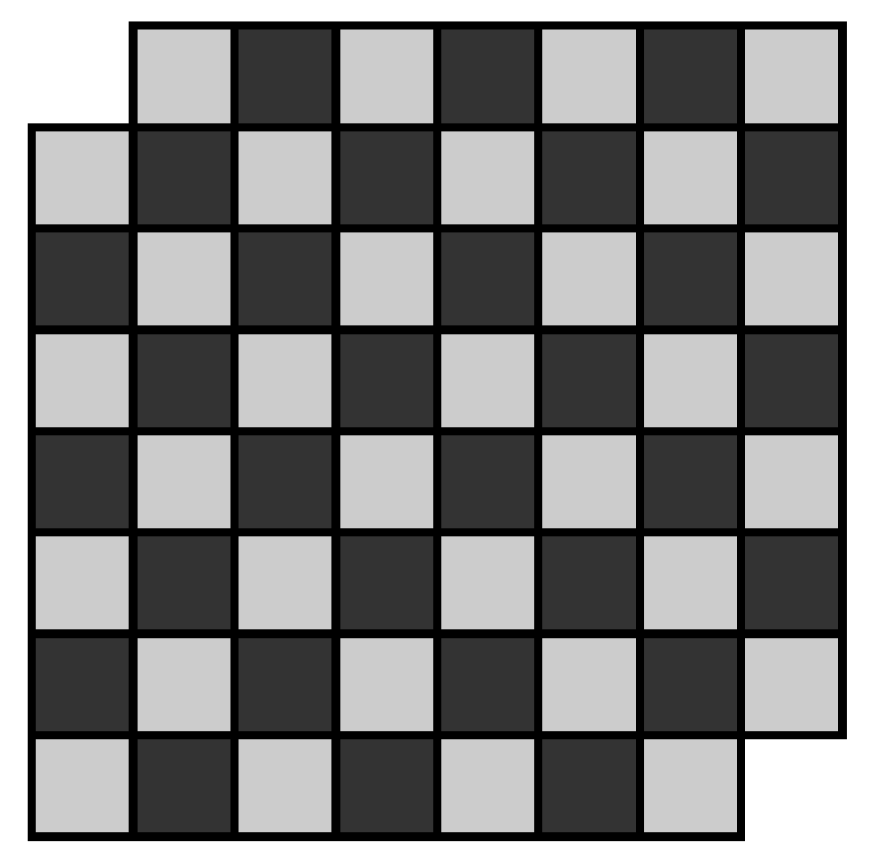
In 1954, Golomb [8] introduced the following famous problem, discussed by others [9,10,11], which motivates the type of colouring arguments used in this article. Remove the two opposite corners of an $8\times 8$ chessboard (see Figure 1). Can the 62 squares be exactly covered by 31 dominoes, with both orientations permitted?

Each domino placed on the chessboard covers exactly one black square and one white square. Thus, if the dominoes exactly tile the board they must cover a total of 31 black squares and 31 white squares. However, the ‘mutilated chessboard’ has 32 white squares and 30 black squares. Thus, the answer is clearly ‘no’.

The focus of this article is the decision problem of whether or not a given set of polyominoes tiles a finite region of the plane called the ‘target region’. The general decision problem is $\mathcal{NP}$-complete [12] and so large problems rapidly become intractable. To help tackle this problem we apply ‘checkerboard’ colouring arguments to the polyominoes and target region, which in certain cases prove the polyominoes do not tile the region. To this end we consider the ‘parity’ of the checkerboard coloured polyominoes or target region, which for a given region is the difference between the number of black squares and the number of white squares. Although checkerboard colouring arguments are common in the literature, a systematic mathematical treatment without using a more theoretical algebraic approach is lacking. The colouring arguments we use yield sufficient, but not necessary conditions for a tiling problem to have no solution, and are generally weaker than the more theoretical tools of Combinatorial Group theory [10,11,13,14,15]. Our main contribution is to tackle this problem algorithmically using colouring arguments, which leads to an efficient numerical method implemented in MATLAB. In addition to developing a systematic method for finding impossible tiling problems we also prove some interesting associated results about polyominoes and their parity values.

Our checkerboard colouring technique identifies impossible tiling problems using polyominoes of arbitrary shape. In graph theory, there is a well-known related approach, which is limited to tiling with dominoes. In that case, black and white squares of the checkerboard coloured region to be tiled are represented by black and white vertices of a graph. A link is made between any two adjacent squares of the region. Then Hall’s marriage theorem gives necessary and sufficient conditions for the existence of a tiling of the region using dominoes, requiring the construction and examination of every possible subset of the white vertices [16].

A checkerboard colouring is not the only way two colours can help prove a tiling problem has no solution. Other colouring schemes have been successfully used in specific cases (see Figure 2 for colouring schemes applied to an $8\times 8$ square [2,8]). However, using two colours, it is only a checkerboard colouring that seems to have wide applicability and hence is amenable to a systematic mathematical description.

The rest of this article has the following structure. In Section 2, we define the basic terminology and concepts. We also prove a number of theoretical results about polyominoes and their parity values. Section 3 concerns what we call a ‘parity violation’, which is a sufficient condition involving the concept of parity for a given set of polyominoes to not tile a target region. We also discuss the combinatorial problem of finding parity violations. In Section 4, we convert the combinatorial problem into the problem of solving a linear Diophantine equation and illustrate our algorithmic approach in Section 5 with some large examples computed in MATLAB. We make some concluding comments regarding possible future work in Section 6. The appendices list some polyomino ‘families’ (Appendix A), and details about our MATLAB solvers for linear Diophantine Equations (Appendix B).

2. Preliminaries

Consider a finite set of F free polyominoes (‘tiles’) in the lattice ${\mathbb{Z}}^2$, denoted ${\left\{P_i\right\}}_{i=1}^F$, $F\ge 1$. We assume the polyominoes are simply-connected, i.e., have no ‘holes’. The area of each polyomino $P_i$ is denoted $c_i$. Consider another arbitrary union of a finite number of edge-connected cells in the lattice ${\mathbb{Z}}^2$ denoted R with area c. We assume R is connected, but not necessarily simply-connected, thus the region R can have ‘holes’. We attempt to tile the target region R with $n_i$ ($n_i\ge 1$) copies of each free polyomino $P_i$, $i=1,\dots ,F$, without ‘gaps’ or tiles overlapping, i.e., we have an exact cover problem. Obviously a necessary condition for a solution to a tiling problem is that the sum of the areas of the tiles must equal the area of the target region, i.e., ${\sum }_{i=1}^F{c}_i{n}_i=c$.

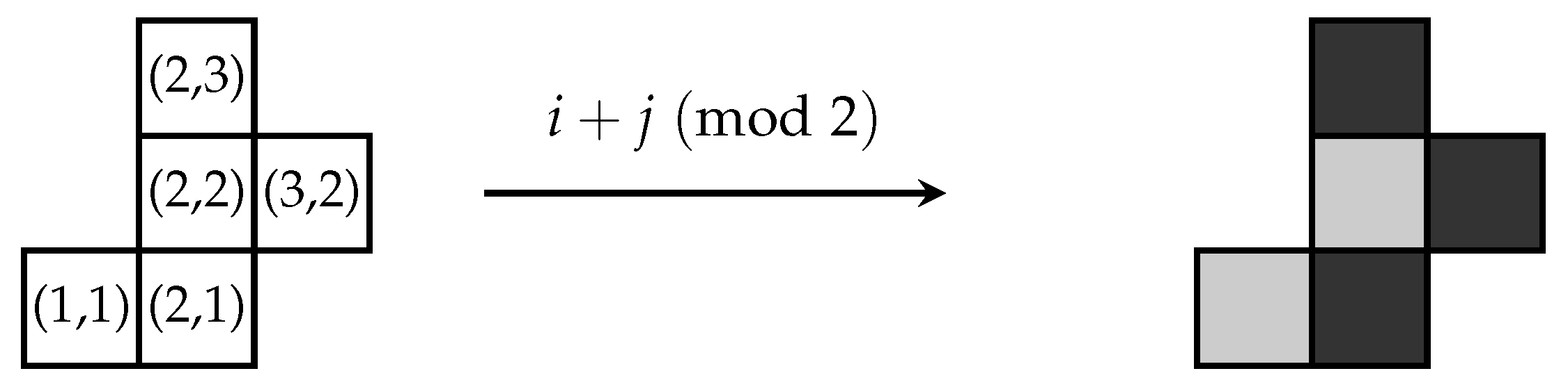
Suppose we colour the cells of a polyomino, or the region we wish to tile, either black or white in such a way that each black cell is edge connected only to white cells and each white cell is edge connected only to black cells. We call this a checkerboard colouring. A checkerboard colouring is rigorously defined using modular arithmetic by identifying each black cell with the number 1 and each white cell with the number 0. If the centre of each cell of a region has coordinates $(i,j)\in {\mathbb{Z}}^2$ then a map $f:{\mathbb{Z}}^2\mapsto \mathbb{Z}$ given by $f(i,j)=i+j\left(\mathrm{mod}2\right)$ defines a checkerboard colouring [17]. If we have $f(i,j)=i+j+1\left(\mathrm{mod}2\right)$ then we reverse the colouring of cells. See Figure 3 for an example (we colour the ‘white’ cells of a checkerboard coloured region light grey, to distinguish them from any holes in the region, which we colour white).

We define the parity (pl. parities) of a checkerboard coloured region as the number of black cells minus the number of white cells. We start each tiling problem by assigning the target region R a fixed checkerboard colouring with parity p, $p\in \mathbb{N}\cup \left\{0\right\}$. A polyomino placed in a checkerboard coloured region R acquires the colouring of the cells it covers. If the parity of a polyomino is non-zero, then it has two parity values $\pm p_i$, $p_i\in \mathbb{N}$, depending on its placement in R. Rotating, reflecting or translating the polyomino in the region may reverse its parity. If a polyomino has zero parity then $p_i=0$. If a polyomino $P_i$ has parity $+p_i$, then its parity becomes $-p_i$ by reversing the colouring of cells (and vice versa).

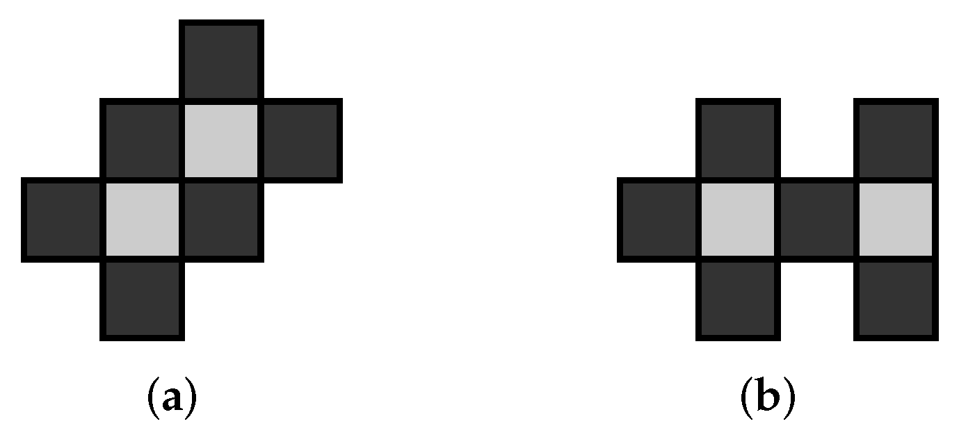
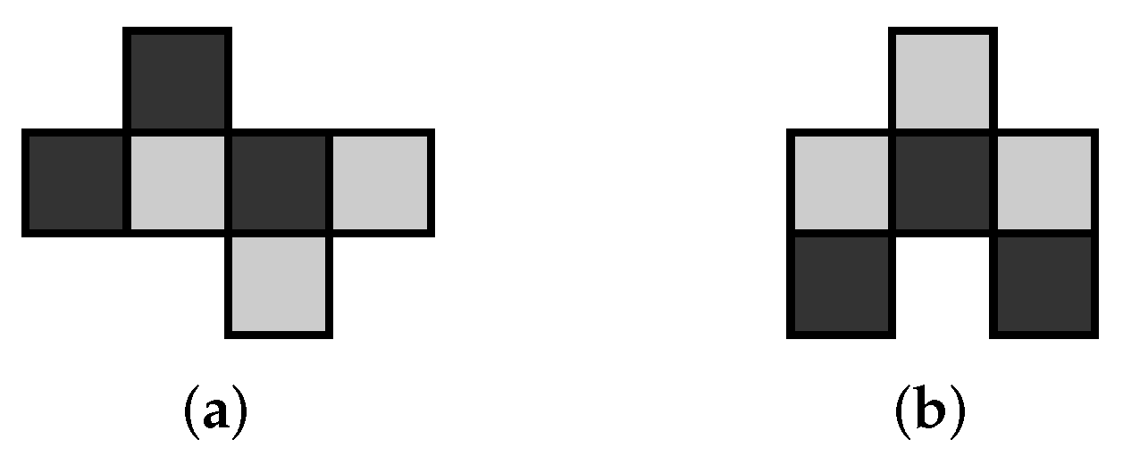
Consider two distinct polyominoes $P_1$ and $P_2$, with the same area n and parities $\pm p_1$ and $\pm p_2$, respectively. Then $P_1$ and $P_2$ are parity equivalent n-ominoes if $p_1=p_2$. Clearly, if $P_1$ and $P_2$ are parity equivalent n-ominoes then $P_1$ can be transformed into $P_2$ (and vice versa) by rearranging the black and white cells. Parity equivalence of n-ominoes is an equivalence relation. An example of parity equivalent 8-ominoes is illustrated in Figure 4.

Consider a polyomino $P_i$ with $b_i$ black cells and $w_i$ white cells. We state the following simple results without proof, as they are immediate consequences of the equations for area ($c_i=b_i+w_i$) and parity ($p_i=b_i-w_i$) of a polyomino (or region) and elementary mathematical induction.

Proposition 1.

(i) 

Parity equivalent n-ominoes have the same number of black squares and the same number of white squares.

(ii) 

Consider the set of all free polyominoes. The parities of polyominoes in this set take on all possible values in $\mathbb{Z}$.

(iii) 

Consider an $m\times n$ rectangle in ${\mathbb{Z}}^2$. If $mn$ is even the parity of the rectangle is 0. If $mn$ is odd the parity is $\pm 1$.

(iv) 

Consider a polyomino $P_i$ with area $c_i$ and parity $\pm p_i$. Then $c_i$ is odd (resp. even) if and only if $\pm p_i$ is odd (resp. even) (we avoid using the term ‘parity’ here in the usual sense to avoid confusion with its alternate definition in this article).

(v) 

Let the number of black cells and white cells of a checkerboard coloured polyomino $P_i$ with area $c_i$ be $b_i$ and $w_i$, respectively. If the parity of $P_i$ is $\pm p_i$, then $b_i=(c_i\pm p_i)/2$, and  $w_i=(c_i\mp p_i)/2$.

As we shall see in later sections, (iii) is useful when we consider the problem of fitting a given set of polyominoes into a rectangle. Additional results for more general polyomino constructions are given in Appendix A, where we give the explicit relationships between area and parity. The results follow from elementary results for sequences and series and mathematical induction.

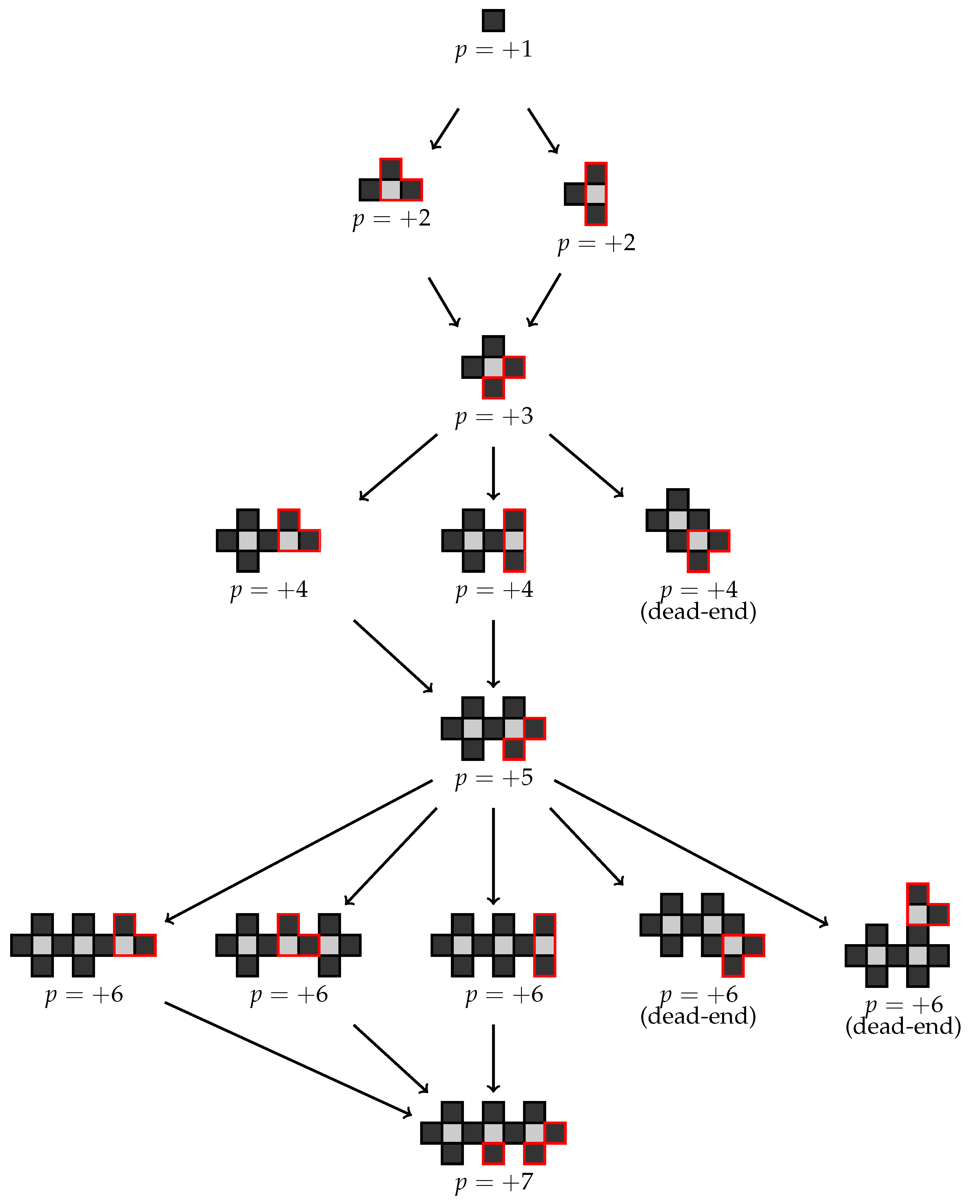
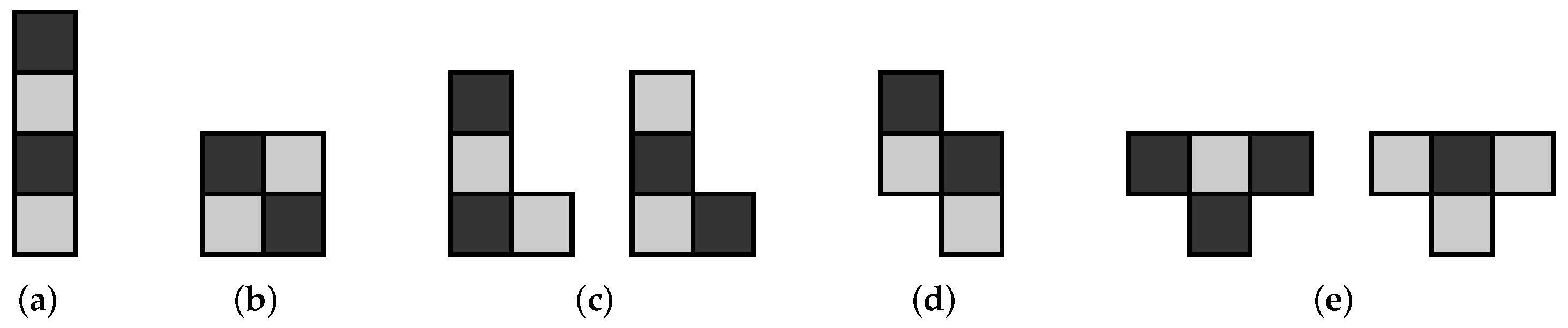
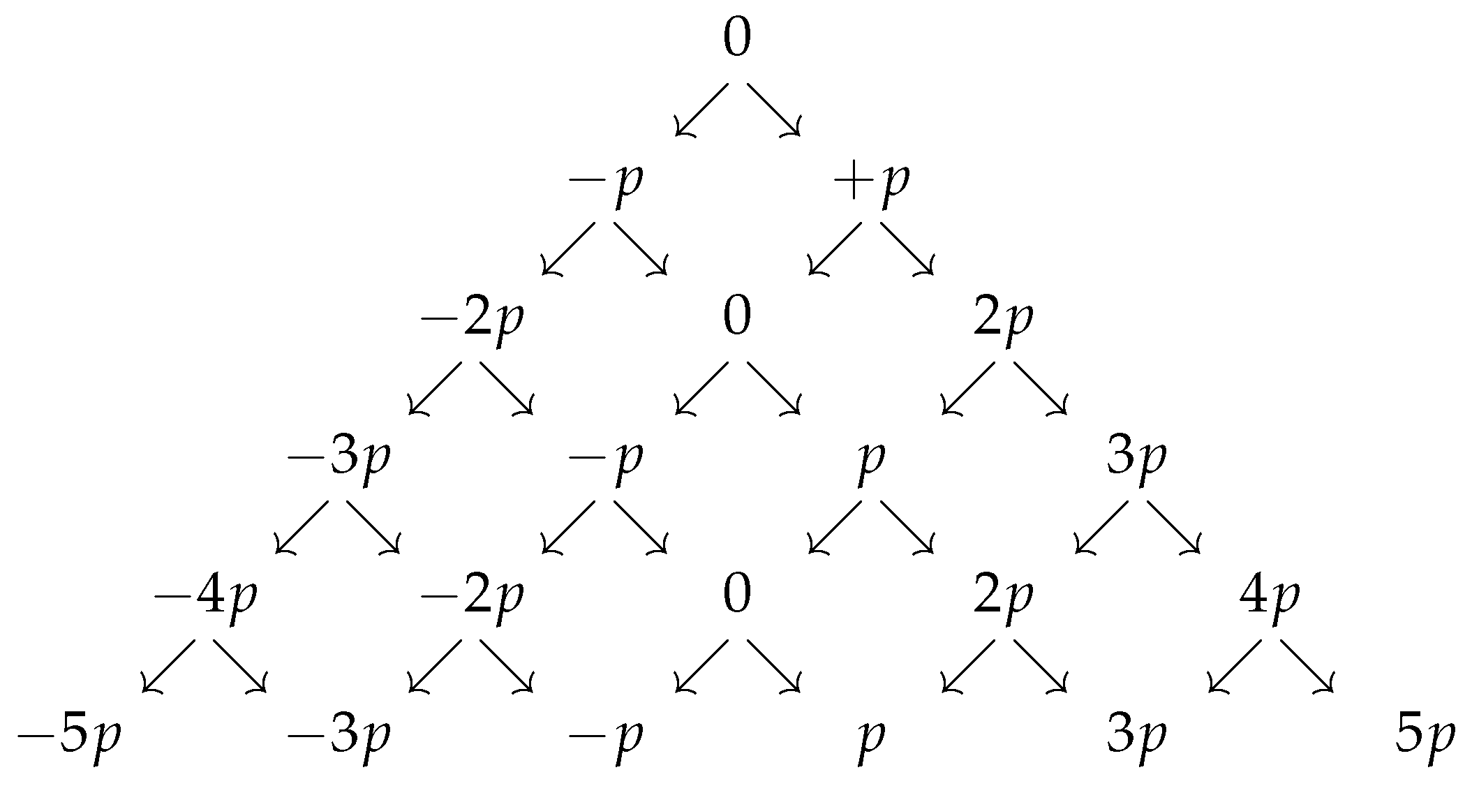
Consider the sequence of free polyomino constructions shown in Figure 5. Starting with a black square, at each stage we add the minimum number of black and white squares to increase the parity by exactly one unit. (If necessary, we allow a re-arrangement of the squares to create all possible parity equivalent n-ominoes at each level, as is the case with the 2nd construction for $p=+6$). From the figure we see that we must initially add a straight trimino , or an L-shaped trimino , (all orientations permitted) and then in the next step a black square, and repeat, yielding the parity sequence $\{+1,+2,+3,\dots \}$. At each level in the construction the shapes are parity equivalent n-ominoes.

The following result clarifies the relationship between the areas and the parities of the polyominoes constructed in Figure 5.

Theorem 1.

Consider the sequence of polyominoes constructed in Figure 5 together with a domino. If the areas of the polyominoes are denoted by $c_p$ with parities $p\in \mathbb{Z}$, then

$$c_p=\left\{\begin{array}{cc}2\left|p\right|-mod(p,2)\hfill & if\left|p\right|\in \mathbb{N},\hfill \\ 2\hfill & ifp=0.\hfill \end{array}\right.$$

(1)

Furthermore, every polyomino in the sequence has minimal area with respect to its parity, or equivalently, maximal parity with respect to its area.

Proof. 

We assume throughout the proof that $p>0$. Similar arguments apply for the case $p<0$ and the result is clearly true for $p=0$ (the case with $p=0$ corresponds to a domino with parity zero). We use induction on p. The result is clearly true for $p=1$. Assume the result is true for p, then we have two cases to consider. If p is even, then $c_p=2p-mod(p,2)=2p$. By construction, we get the next polyomino in the sequence with a parity of $p+1$ by adding a single black square, yielding an area of $2p+1=2(p+1)-1=2(p+1)-mod(p+1,2)$ as $p+1$ is odd. If p is odd, then $c_p=2p-mod(p,2)=2p-1$. By construction we get the next polyomino in the sequence with a parity of $p+1$ by adding two black squares and one white square. So the area becomes $c_p=2p-1+3=2(p+1)=2(p+1)-mod(p+1,2)$ as $p+1$ is even.

At each stage of the construction procedure in Figure 5 we add the least number of black and white squares to increase the parity by one unit. If the parity is odd, no white squares are accessible, so we must add either an L-shaped trimino or a straight trimino. There are various ways to do this and the resulting even parity constructions are parity equivalent n-ominoes. Although all the odd parity polyominoes have minimal area with respect to their parity, some of them cannot be continued in the sequence (labelled ‘dead-end’). If a white square is not accessible, then the only way the parity can be increased by one unit is by adding one white square and two black squares, resulting in a polyomino that no longer has minimal area (e.g., the third polyomino with $p=+4$). Even if a white square is accessible, we cannot always add a single black square to increase the parity by a single unit. For example, in the fifth polyomino construction with $p=+6$, adding a black square to the single accessible white square is not permitted as this yields a shape that is not simply-connected, contradicting our definition of a polyomino. Thus, in this case, and similar ones, the only way to legitimately increase the parity is by adding three squares (two black and one white), again resulting in a polyomino that no longer has minimal area. As we progress down more levels of the tree the same pattern of polyomino constructions continue, although when the parity is even we get more parity equivalent n-ominoes.

The sequence of polyominoes also have maximal parity with respect to their area. If this were not true then it would be possible to reduce the area of a polyomino without changing its parity. To do this we would have to remove an equal number of black squares and white squares. However, we cannot remove a single white square from any of the polyominoes as the resulting shape would no longer be simply-connected, contradicting our definition of a polyomino.       □

Theorem 1 leads to a simple upper bound for the parity of a polyomino with respect to its area as shown in the following corollary.

Corollary 1.

Consider a polyomino $P_i$ with area $c_i$ and parity $\pm p_i$ $(p_i\in \mathbb{N})$. Then for all $p_i\in \mathbb{N}$ we have

$$p_i\le \left\{\begin{array}{cc}{c}_i/2\hfill & if{p}_{i}iseven,\hfill \\ (c_i+1)/2\hfill & if{p}_{i}isodd.\hfill \end{array}\right.$$

Proof. 

From Theorem 1 the least possible area for a polyomino $P_i$ with area $c_i$ and parity $\pm p_i$ is given by

$$c_{\min }=2p_i-mod(p_i,2)\le c_i\mathrm{for}\mathrm{all}{p}_i\in \mathbb{N},$$

and if the parity is zero then $c_i\ge 2$. Thus, for all $p_i\in \mathbb{N}$

$$\begin{array}{cc}\hfill p_i& \le \frac{c_i+mod(p_i,2)}{2}=\left\{\begin{array}{cc}{c}_i/2\hfill & \mathrm{if}{p}_i\mathrm{is}\mathrm{even},\hfill \\ (c_i+1)/2\hfill & \mathrm{if}{p}_i\mathrm{is}\mathrm{odd},\hfill \end{array}\right.\hfill \end{array}$$

as required.       □

A proof of the less sharp result $p_i\le (c_i+1)/2$ is given in ([18], p. 42) using a different argument.

3. Parity Violations

3.1. A Sufficient Condition for a Non-Tileable Region

We describe a simple sufficient condition for a tiling problem to have no solution based on the parity of the target region and the parities of the tiles.

We attempt to tile a region R with parity p using F free polyominoes ${\left\{P_i\right\}}_{i=1}^F$ with copies ${\left\{n_i\right\}}_{i=1}^F$, $n_i\ge 1$. Assume the polyominoes have parity values ${\{\pm p_i\}}_{i=1}^F$ (if the parity value is zero then for ease of notation the parity is still represented as $\pm p_i$). Denote the multiset of all possible sums of $N={\sum }_{i=1}^F{n}_i$ parity values by ${\left\{s_j\right\}}_{j=1}^M$, $M\ge 1$. The following elementary result is key to the arguments that follow:

Proposition 2.

A necessary (but not sufficient) condition for the polyominoes to tile a region R is that $s_j=p$ for at least one $j\in \{1,2,\dots ,M\}$.

Proof. 

Assume the polyominoes ${\left\{P_i\right\}}_{i=1}^N$ tile the target region R. For each polyomino $P_k$ with $b_k$ black cells and $w_k$ white cells the parity is given by $\pm p_k=b_k-w_k$ and thus there exists a $j\in \{1,2,\dots ,M\}$ such that

$$s_j=\sum _{k=1}^N(\pm p_k)=\sum _{k=1}^N(b_k-w_k)=\sum _{k=1}^N{b}_k-\sum _{k=1}^N{w}_k=b-w=p.$$

 □

When none of the possible parity sums equals the parity of the target region we call this a parity violation which implies it is impossible for the given polyominoes to tile the target region.

Example 1.

Consider the problem of tiling the target regions R in Figure 6 with three dominoes, both orientations permitted. The parity of a domino is zero and thus it is always the case that $s_j=0$ for pure domino tiling problems. Furthermore, the parities of the checkerboard coloured target regions in Figure 6a,b are zero, so the necessary condition of Proposition 2 is always satisfied. However, Figure 6a illustrates that this condition is not sufficient.

We consider some simple tiling problems that lead to a parity violation.

Example 2.

Apply a checkerboard colouring to the five free tetrominoes, yielding seven free checkerboard coloured tetrominoes, illustrated in Figure 7.

Any rectangle tiled by the five free tetrominoes must have an area of 20 cells, and as the area is even the parity of the target region must be zero; see Proposition 1 (iii). From Figure 7 we see that the sum of parities of the five tetrominoes is given by $s_1=+2$ or $s_2=-2$, thus from Proposition 2 we conclude that the tetrominoes do not tile any rectangle. This result is proved in ([2], p. 17) using a similar checkerboard colouring argument to the one presented here, but without parity considerations.

Example 3.

Consider the problem of tiling any rectangle with the 35 free hexominoes [2]. Any rectangle tiled by these polyominoes must have an area of $35\times 6=210$ cells, thus the parity of the target region is zero. Of the 35 hexominoes, 11 polyominoes have a parity of $\pm 2$, while the remaining 24 polyominoes have a parity of zero. Observe that the sum of 11 numbers from the set $\{-2,+2\}$ can never equal zero, thus application of Proposition 2 yields that the 35 free hexominoes can never tile a rectangle. This result is proved in ([2], p. 10) using a similar checkerboard colouring argument to the one presented here, but without parity considerations.

Example 4.

Is it possible for 15 T-shaped tetrominoes (see Figure 8b) to tile the checkerboard coloured region shown in Figure 8a? The target region is the 5th polyomino in the ‘diamond-shapes’ family (see Appendix A), but with a square removed from the middle. Thus, the target region has area $c_5-1=36+25-1=60$ and parity $p_5+1=11+1=+12$. The parity values of the tetrominoes are $\pm 2$. However, it is not possible for a one-dimensional walk along the integers with 15 steps from $\{-2,+2\}$ to arrive at $+12$. Thus, the answer is ‘no’.

These simple examples illustrate that when using a parity violation to prove a tiling problem has no solution we must solve a combinatorial problem. We need to consider all possible sums of the parities of the polyominoes and verify that none of them equals the parity of the region we wish to tile.

3.2. Combinatorial Considerations

In the practical application of Proposition 2 to large tiling problems we must compute all possible parity sums for a given set of polyominoes, i.e.,:

(${\mathrm{P}}_1$)  find all possible sums ${\left\{s_j\right\}}_{j=1}^M$ given by:

$$\begin{array}{c}\hfill \left\{\begin{array}{cc}\hfill & n_1\mathrm{elements}\mathrm{drawn}\mathrm{from}\{-p_1,+p_1\},\mathrm{with}\hfill \\ \hfill & n_2\mathrm{elements}\mathrm{drawn}\mathrm{from}\{-p_2,+p_2\},\mathrm{with}\hfill \\ \hfill & ⋮⋮\hfill \\ \hfill & n_F\mathrm{elements}\mathrm{drawn}\mathrm{from}\{-p_F,+p_F\},\hfill \end{array}\right.\end{array}$$

where $n_i\in \mathbb{N}$ and $p_i,p\in \mathbb{N}\cup \left\{0\right\}$, for $i=1,2,\dots ,F$.

With N polyominoes we have $2^N$ different ways to sum the parity values, assuming the parities are distinct and non-zero. However, it is often the case that many of the polyominoes have the same parity value, or are zero, which reduces the number of possible sums of parities. We define the parity problem as the decision problem of whether any of the parity sums equals p. This problem is similar to the general subset sum problem, which is $\mathcal{NP}$-complete [19]. The tree diagram in Figure 9 illustrates the possible ways of adding five elements from $\{-p,+p\}$ (here, the arrow ↘ denotes adding $+p$ while the arrow ↙ denotes adding $-p$).

The following are some related results:

Proposition 3.

(i) 

All possible sums of $n_k$ elements drawn from $\{-p_k,+p_k\}$ are given by

$$s_j=p_k(n_k-2j),n_k\ge 0,j=0,1,\dots ,n_k.$$

(ii) 

The number of sums we can form in the combinatorial problem $\left(P_1\right)$ is given by

$$M=\prod _{k=1}^F(1+n_k).$$

(iii) 

Consider a tiling problem using $n_k$ copies of each free polyomino $P_k$ for $k=1,2,\dots ,F$, where each polyomino has $z_k$ parity equivalent polyominoes. If the tiling problem yields a parity violation then the number of equivalent parity violation problems is given by:

$$\prod _{k=1}^F\left(\begin{array}{c}{z}_k+n_k-1\\ n_k\end{array}\right).$$

Proof. 

(i)

If the number of occurrences of $-p_k$ in the sum is j, $j\in \{0,1,\dots ,n_k\}$, then the number of occurrences of $+p_k$ in the sum is $n_k-j$, yielding the sums

$$s_j=j(-p_k)+(n_k-j)(+p_k)=p_k(n_k-2j),\mathrm{for}j=0,1,\dots ,n_k.$$

(ii)

From (i) we see that the total number of sums of $n_k$ elements drawn from the set $\{-p_k,+p_k\}$ is given by $1+n_k$. The result then follows if we apply the Fundamental Counting Principle over all sets for $k=1,\dots ,F$.

(iii)

The number of combinations of $z_k$ parity equivalent polyominoes taken $n_k$ at a time with repetition is given by $\left(\begin{array}{c}{z}_k+n_k-1\\ n_k\end{array}\right)$ ([20], p. 36). Thus, applying the Fundamental Counting Principle again over all F equivalence classes yields the result.

□

Proposition 3 (iii) is illustrated in the following example:

Example 5.

Consider the problem of tiling the $8\times 8$ square with the following polyominoes

,all orientations permitted, using $n_1=3$, $n_2=2$, and $n_3=3$ copies, respectively. The target region has a parity of zero, and the total area of the tiles is $3\left(4\right)+2\left(8\right)+3\left(12\right)=64$ as required. The polyominoes have parity values of $0,\pm 4,\pm 6$, respectively, and it is easily verified that this problem yields a parity violation. We note that $z_1=4$, $z_2=3$, and $z_3=5$ (see Figure 5 and Figure 7). Thus, from Proposition 3 (iii) the number of equivalent parity violation problems is given by

$$\prod _{i=1}^3\left(\begin{array}{c}{z}_i+n_i-1\\ n_i\end{array}\right)=\left(\begin{array}{c}6\\ 3\end{array}\right)\left(\begin{array}{c}4\\ 2\end{array}\right)\left(\begin{array}{c}7\\ 3\end{array}\right)=4200.$$

The parity sums $s_j$ are bounded by the maximum and minimum possible sums of parity values, i.e.,

$$\sum _{k=1}^F(-p_k)\le s_j\le \sum _{k=1}^F(+p_k),j=1,\dots ,M.$$

(2)

Thus, we obtain a parity violation if p lies outside the bounds for $s_j$ given in Equation (2). In this case we say we have a trivial parity violation as there is no combinatorial problem to solve. A simple example of this type is when the parity of the target region is non-zero and the parities of all the tiles are zero (as is the case with the first example in this article involving a mutilated checkerboard). As a result, any region that is tileable by dominoes must have zero parity, i.e., the number of black squares must equal the number of white squares. Another example of a trivial parity violation is given below:

Example 6.

Consider the problem of tiling the 4th member of the ‘diamond-shapes’ (see Appendix A) using five L-shaped tetrominoes and seven straight triminoes , all orientations permitted. The tetrominoes and triminoes have parity values of zero and $\pm 1$, respectively. The target region has a parity of $+9$ and an area of $41$. The total area of the tiles is $5\left(4\right)+7\left(3\right)=41$ as required, however, the parity of the target region lies outside the bounds for the maximum possible sum of the parities of the tiles, namely $\pm 7$, which implies we have a trivial parity violation for this problem.

4. Linear Diophantine Equation Approach

In this section, we convert the combinatorial problem of finding parity violations into the problem of solving linear Diophantine equations. The theoretical results form the basis for a practical algorithm implemented in MATLAB for identifying all possible parity violations of a given tiling problem, presented in Section 5.

Consider the problem of whether F free polyominoes ${\left\{P_i\right\}}_{i=1}^F$ with areas $c_i$ and $n_i$ ($n_i\ge 1$) copies of each polyomino $P_i$ are able to tile a target region R with area c. The total number of polyominoes used is $N:={\sum }_{i=1}^F{n}_i$. If the number of copies of each polyomino is not specified then we have the following linear Diophantine equation in F unknowns ${\left\{n_i\right\}}_{i=1}^F$ to solve for:

$$c_1{n}_1+c_2{n}_2+\cdots +c_F{n}_F=c,\mathrm{for}{n}_i\in \mathbb{N},i=1,\dots ,F.$$

(3)

A well-known classical result (e.g., see (([21], p. 30)) is that a necessary condition for the existence of integer solutions (and hence also positive integer solutions) of (3) is

$$gcd(c_1,c_2,\dots ,c_F)\mid c,$$

(4)

where $gcd(c_1,c_2,\dots ,c_F)$ denotes the greatest common divisor of the numbers $c_1,c_2,\dots ,c_F$. Now denote the solutions of (3) by the set of F-tuples

$$S_c:=\{(n_1,n_2,\dots ,n_F):n_i\in \mathbb{N}\},$$

(5)

which may be empty. The subscript c of $S_c$ indicates that the solution set depends on c in (3).

Assume the target region R has a fixed parity $p\in \mathbb{N}\cup \left\{0\right\}$ and the polyominoes $P_i$ have parities $\pm p_i$, $p_i\in \mathbb{N}\cup \left\{0\right\}$ and W.L.O.G. the first r polyominoes, $0\le r\le F-1$ have zero parity.

In the arguments below we will need the following simple lemma:

Lemma 1.

Let $\mathcal{O}$ and $\mathcal{E}$ denote the set of odd and even integers, respectively. Then for all $a_i,b_i,c_i\in \mathbb{Z}$

$$\sum _{i=1}^M(a_i+b_i)c_i\in \mathcal{O}(resp.\mathcal{E})\iff \sum _{i=1}^M(a_i-b_i)c_i\in \mathcal{O}(resp.\mathcal{E}).$$

Proof. 

Recall from the elementary properties of odd and even numbers that the sum of two numbers $a+b$ is odd (resp. even) if and only if the difference $a-b$ is odd (resp. even). After setting $a:={\sum }_{i=1}^M{a}_i{c}_i$ and $b:={\sum }_{i=1}^M{b}_i{c}_i$ the result follows.    □

The following theorem is the theoretical basis of Algorithm 1 presented in Section 4:

Theorem 2.

Let the variable $a_i\in \mathbb{N}\cup \left\{0\right\}$ denote how many of the $n_i$ elements drawn from $\{-p_i,+p_i\}$ are $+p_i$, $0\le a_i\le n_i$, $i=r+1,r+2,\dots ,F$. A solution $(n_1,n_2,\dots ,n_F)$ of the linear Diophantine Equation (3) (if it exists) yields a parity violation if and only if one of the following mutually exclusive conditions holds:

(i) 

$gcd(p_{r+1},p_{r+2},\cdots ,p_F)\cancel{|}k$, where

$$k:=(p+p_{r+1}{n}_{r+1}+p_{r+2}{n}_{r+2}+\dots +p_F{n}_F)/2\in \mathbb{Z}.$$

(ii) 

$gcd(p_{r+1},p_{r+2},\dots ,p_F)\mid k$ but there is no solution to the following linear Diophantine equation in $F-r$ unknowns ${\left\{a_i\right\}}_{i=r+1}^F$:

$$p_{r+1}{a}_{r+1}+p_{r+2}{a}_{r+2}+\dots +p_F{a}_F=k.$$

(iii) 

There exists one or more solutions to the linear Diophantine equation in (ii), but none of the solutions satisfy the bounds

$$0\le a_i\le n_i,a_i\in \mathbb{N}\cup 0,i=r+1,r+2,\dots ,F.$$

Proof. 

To find possible parity violations we need an equation that matches the sum of the parities of the tiles to the parity of the target region. Our starting point is the parity problem of Section 3.2. As we have $a_i$ choices for how many of the $n_i$ elements drawn from $\{-p_i,+p_i\}$ are $+p_i$, we must have $n_i-a_i$ choices of $-p_i$, $0\le a_i\le n_i$, $i=r+1,r+2,\dots ,F$ (recall, the parities of the first r polyominoes are zero). Then the equation $s_j=p$ becomes

$$\begin{array}{cc}\hfill & (+p_{r+1})a_{r+1}+(-p_{r+1})(n_{r+1}-a_{r+1})+(+p_{r+2})a_{r+2}+(-p_{r+2})(n_{r+2}-a_{r+2})+\hfill \\ \hfill & \cdots +(+p_F)a_F+(-p_F)(n_F-a_F)=p,\hfill \end{array}$$

or after some simplification

$$\begin{array}{cc}\hfill & 2p_{r+1}{a}_{r+1}+2p_{r+2}{a}_{r+2}+\cdots +2p_F{a}_F\hfill \\ \hfill & =p+p_{r+1}{n}_{r+1}+p_{r+2}{n}_{r+2}+\cdots +p_F{n}_F,\mathrm{for}r\in \{0,1,\dots ,F-1\},\hfill \end{array}$$

(6)

which is a linear Diophantine equation in $F-r$ unknowns ${\left\{a_i\right\}}_{i=r+1}^F$ (if all F polyominoes have zero parity then we obtain a trivial parity violation if $p\ne 0$).

We claim that the right hand side of Equation (6) is an even number. To show this we prove that p is even (resp. odd) exactly when $p_1{n}_1+p_2{n}_2+\cdots +p_F$ is even (resp. odd), and thus from the elementary property that the sum of two even (resp. odd) numbers is even the result will follow. Recall that we denote the number of black and white squares in a polyomino $P_i$ by $b_i$ and $w_i$, respectively. Assume p is even (resp. odd), then from Proposition 1 (iv) we know c is even (resp. odd) and hence from (3)

$$c_1{n}_1+c_2{n}_2+\cdots +c_F{n}_F=(b_1+w_1)n_1+(b_2+w_2)n_2+\cdots +(b_F+w_F)n_F$$

is also even (resp. odd). However, from Lemma 1

$$\begin{array}{cc}\hfill & (b_1-w_1)n_1+(b_2-w_2)n_2+\cdots +(b_F-w_F)n_F\hfill \\ \hfill & =0+0+\cdots +p_{r+1}{n}_{r+1}+p_{r+2}{n}_{r+2}+\cdots +p_F{n}_F\hfill \end{array}$$

is also even (resp. odd), and so the result follows. As a consequence we can safely divide through by 2 in Equation (6) yielding

$$\begin{array}{cc}\hfill & p_{r+1}{a}_{r+1}+p_{r+2}{a}_{r+2}+\cdots +p_F{a}_F=k\in \mathbb{Z}.\hfill \\ \hfill & \mathrm{where}k:=(p+p_{r+1}{n}_{r+1}+p_{r+2}{n}_{r+2}+\cdots +p_F{n}_F)/2,\hfill \\ \hfill & \mathrm{for}0\le a_i\le n_i,a_i\in \mathbb{N}\cup 0,i=r+1,r+2,\dots ,F.\hfill \end{array}$$

(7)

The appropriate necessary condition for the existence of integer solutions (and hence also for non-negative integer solutions) of Equation (7) is

$$gcd(p_{r+1},p_{r+2},\dots ,p_F)\mid k.$$

(8)

So for each value of k, depending on a solution from (5), we have the (possibly empty) solution set given by

$$S_k:=\{(a_{r+1},a_{r+2},\dots ,a_F):a_i\in \mathbb{N}\cup \left\{0\right\}\}.$$

So if either the gcd condition (8) is not satisfied, or, when the gcd condition is satisfied, but the linear Diophantine Equation (7) has no solution, then the solution $(n_1,n_2,\dots ,n_F)$ of the linear Diophantine Equation (3) yields a parity violation. Furthermore, in the case that the linear Diophantine Equation (7) has one or more solutions, we also get a parity violation if none of the solutions in the set $S_k$ satisfy the bounds (7).       □

Algorithm 1 An algorithm for finding all possible parity violations of a tiling problem

1: Input ${\left\{p_i\right\}}_{i=1}^F$, ${\left\{c_i\right\}}_{i=1}^F$, p, and c. Parities $p_1,p_2,\dots ,p_r$ are zero ($0\le r\le F-1$). 2: Identify r from the user input of ${\left\{p_i\right\}}_{i=1}^F$. 3: $S\leftarrow$ positive integer solutions of (3), computed using DIOPHANTINE_ND_POSITIVE 4: $ns\leftarrow$ length of S 5: $S1\leftarrow \varnothing$ 6: $S2\leftarrow \varnothing$ 7: for$i=1$ to $ns$ do 8:      $si\leftarrow$ith solution of S 9:      $sp\leftarrow$ entries of $si$ corresponding to nonzero parities {solution of form      ($n_{r+1},n_{r+2},\dots ,n_F$)} 10:      $max\_sum\leftarrow$ maximum possible sum of parities using (2) 11:      if $max\_sum<p$ then 12:           Add $si$ to $S1$ 13:           Continue {Go to next iteration in For Loop} 14:      end if 15:      $k\leftarrow (p+p_{r+1}{n}_{r+1}+p_{r+2}{n}_{r+2}+\cdots +p_F{n}_F)/2$ as in (7) 16:      $T\leftarrow$ non-negative integer solutions of (7), computed using DIOPHANTINE_ND_NONNEGATIVE 17:      $nt\leftarrow$ length of T 18:      $flag\leftarrow 2$ 19:      for $j=1$ to $nt$ do 20:           $tj\leftarrow$jth solution of T 21:           if all $tj\le sp$ then 22:                $flag\leftarrow 0$ 23:                break {Leave current For Loop} 24:           end if 25:      end for 26:      if $flag==2$ then 27:           Add $si$ to $S2$ 28:      end if 29: end for

5. Numerical Results

In this section, we illustrate the theoretical approach for finding large impossible tiling problems with an efficient algorithm implemented in MATLAB.

The open-source MATLAB (R2021b) programs used in this section are freely available in a repository, POLYOMINO_PARITY (v2.0.0) [22], and run on a Mac Pro (OS X 12.0.1) with 32 GB of memory and a 3.5 GHz 6-core Intel Xeon E5. We describe an algorithm based on Theorem 2 guaranteed to find all possible parity violations of a given tiling problem. To this end we must solve linear Diophantine equations in n variables ${\sum }_{i=1}^n{a}_i{x}_i=b$, where the coefficients $a_i$ and the right hand side value b are strictly positive integers. We wish to find all solutions $x_i$ which are either nonnegative or strictly positive integers. Under the assumptions on a and b, there are only a finite number of nonnegative or strictly positive integer solutions. We constructed the MATLAB functions DIOPHANTINE_ND_NONNEGATIVE and DIOPHANTINE_ND_POSITIVE with the syntax

•   x = Diophantine_nd_nonnegative(a,b)
•   x = Diophantine_nd_positive(a,b)

which accept the coefficient n-vector a and right hand side b of a Diophantine equation, and return the set of solutions in an $n\times k$ array x. Further details are given in Appendix B.

Our starting point is a given set of F free polyominoes ${\left\{P_i\right\}}_{i=1}^F$ with areas ${\left\{c_i\right\}}_{i=1}^F$. The numbers of copies of the free polyominoes ${\left\{n_i\right\}}_{i=1}^F$ is initially left unspecified. Once we have chosen a target region (e.g., from the families of polyominoes in Appendix A) we use Algorithm 1 implemented in MATLAB using the function PV_SEARCH with the syntax

•   [ S1, S2 ] = pv_search ( par, ord, p, c ),

which accepts the positive (or zero) parities of the polyominoes par, the areas of the polyominoes ord, and the parity p and area c of the target region. PV_SEARCH returns S1, the solutions to the area equation yielding trivial parity violations and S2, the solutions to the area equation yielding non-trivial parity violation.

We illustrate this algorithm with several examples. In each problem we use PV_SEARCH to find all possible parity violations. In the first three examples we also use the open-source MATLAB programs, POLYOMINOES (v2.0.0) [23] (described in [24]), to yield successful tiling of the target regions concerned, However, there were many possible solutions and we made no attempt to enumerate them all, even for a particular choice of ${\left\{n_i\right\}}_{i=1}^F$.

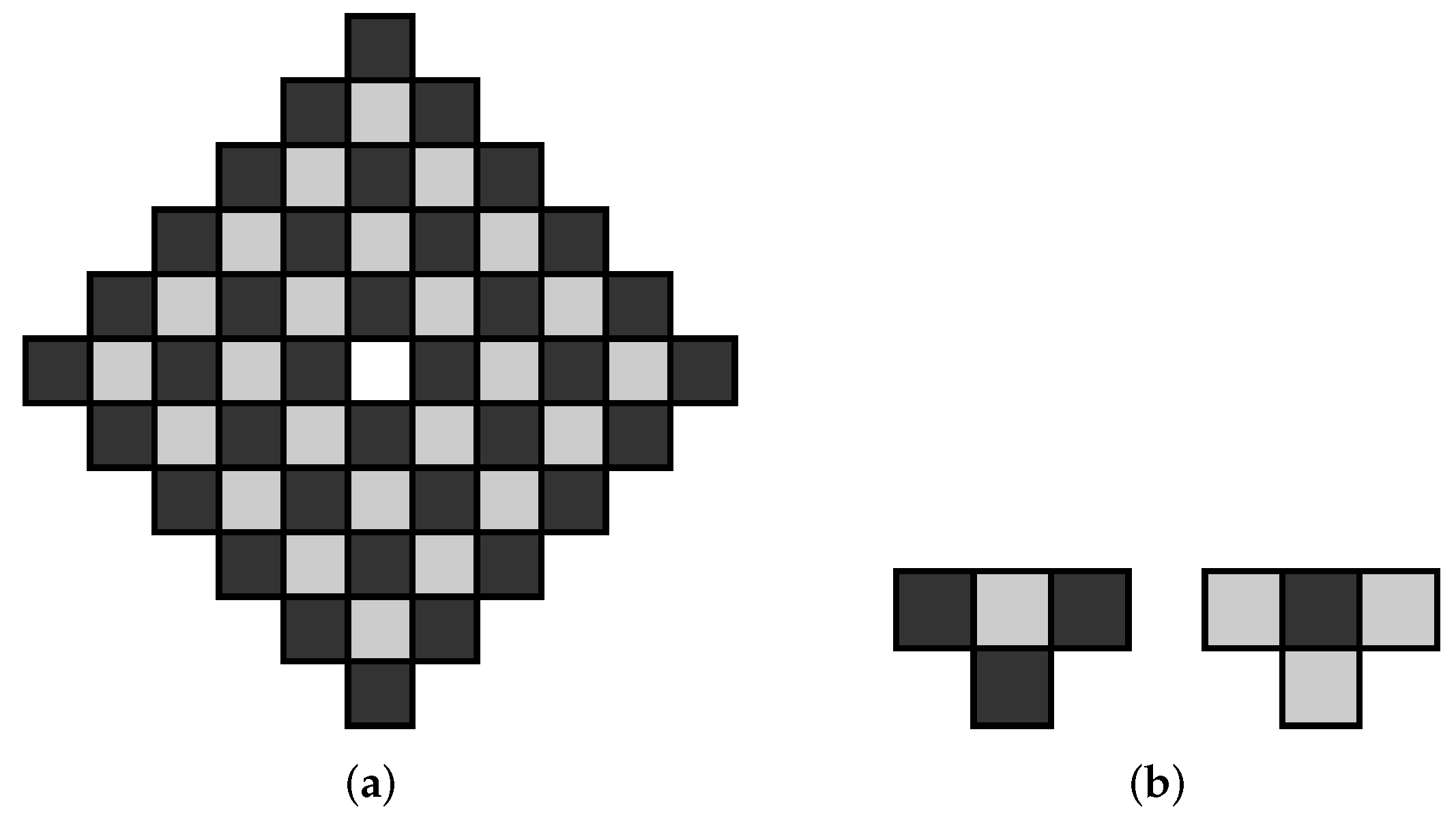
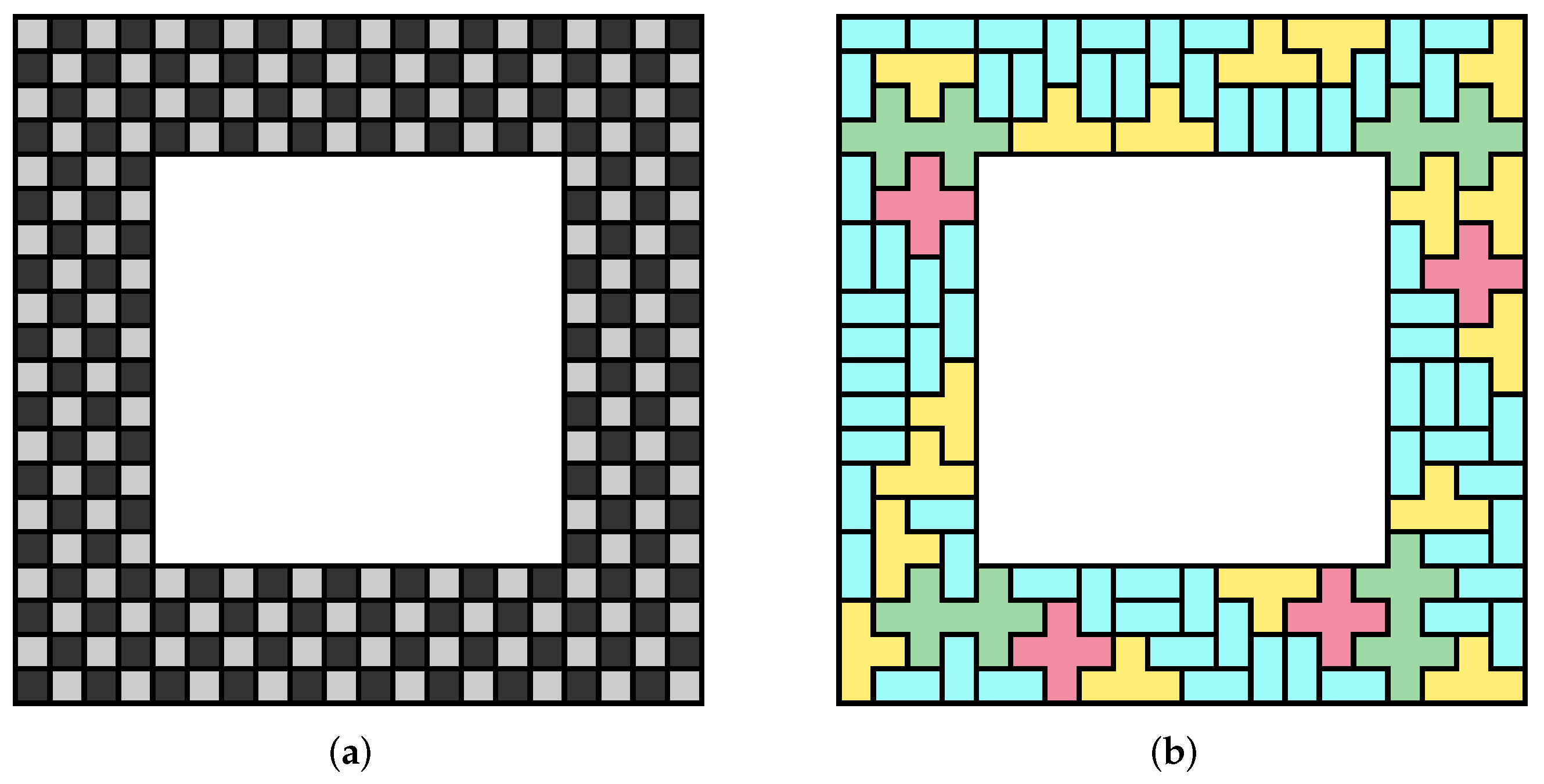
Example 7.

We consider the problem of tiling the checkerboard coloured region shown in Figure 10a with copies of

.

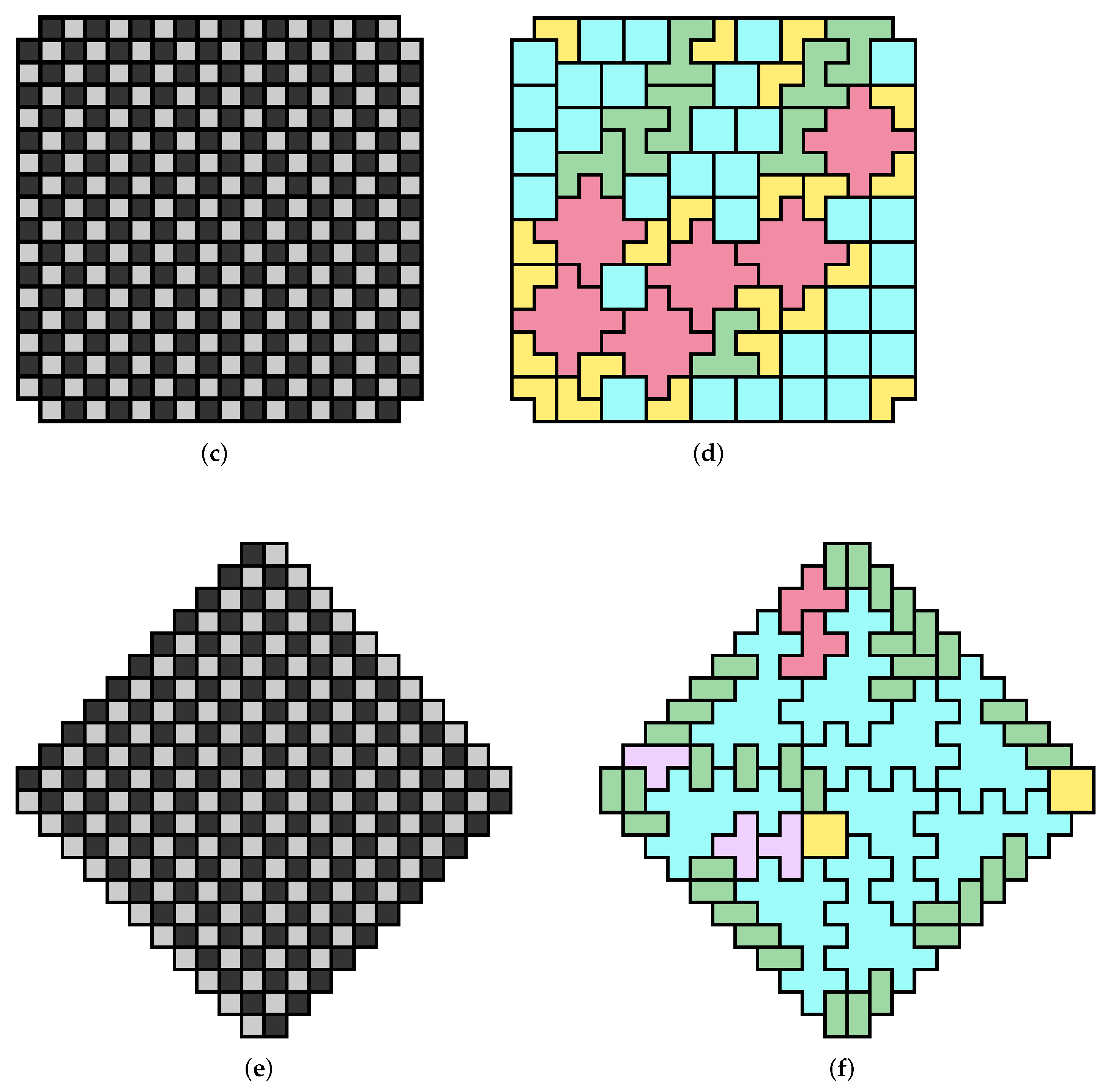
The tiles have parities $\{0,\pm 2,\pm 3,\pm 5\}$ and areas $\{2,4,5,9\}$, respectively. The target region (see Appendix A) has an area of $256$ and a parity value of zero. Solving the linear Diophantine equation $2n_1+4n_2+5n_3+9n_4=256$ yields $6896$ solutions.PV_SEARCHfound in $1.24$ s that only $26$ of these solutions yielded parity violations (see

Table 1. The 26 solutions of $2n_1+4n_2+5n_3+9n_4=256$ yielding a parity violation.

#	1	2	3	4	5	6	7	8	9	10	11	12	13
$n_1$	4	9	13	18	22	27	31	36	40	45	49	54	58
$n_2$	1	2	1	2	1	2	1	2	1	2	1	2	1
$n_3$	2	1	2	1	2	1	2	1	2	1	2	1	2
$n_4$	26	25	24	23	22	21	20	19	18	17	16	15	14
#	14	15	16	17	18	19	20	21	22	23	24	25	26
$n_1$	63	67	72	76	81	85	90	94	99	103	108	112	117
$n_2$	2	1	2	1	2	1	2	1	2	1	2	1	2
$n_3$	1	2	1	2	1	2	1	2	1	2	1	2	1
$n_4$	13	12	11	10	9	8	7	6	5	4	3	2	1

):

With the particular choice $(n_1,n_2,n_3,n_4)=(66,17,4,4)$ the polyominoes tile the target region (see Figure 10b).

Example 8.

We consider the problem of tiling the checkerboard coloured region shown in Figure 10c with copies of

.

We note that these tiles have parities $\{0,\pm 1,\pm 2,\pm 5\}$ and areas $\{4,3,6,13\}$, respectively. The target region (see Appendix A) has an area of 320 and a parity value of zero. Solving the linear Diophantine equation $4n_1+3n_2+6n_3+13n_4=320$ yields 5158 solutions. PV_SEARCH found in $1.50$ s that only six of these solutions yielded parity violations (see

Table 2. The six solutions of $4n_1+3n_2+6n_3+13n_4=320$ yielding a parity violation.

#	1	2	3	4	5	6
$n_1$	3	16	29	42	55	68
$n_2$	1	1	1	1	1	1
$n_3$	1	1	1	1	1	1
$n_4$	23	19	15	11	7	3

):

With the particular choice of $(n_1,n_2,n_3,n_4)=(32,22,8,6)$ the polyominoes tile the target region (see Figure 10d).

Example 9.

We consider the problem of tiling the checkerboard coloured region shown in Figure 10e with copies of .

We note that these tiles have parities $\{0,0,\pm 2,\pm 1,\pm 8\}$ and areas $\{2,4,4,5,18\}$, respectively. The target region (see Appendix A) has an area of 264 and a parity value of zero. Solving the linear Diophantine equation $2n_1+4n_2+4n_3+5n_4+18n_5=264$ yields 51,923 solutions. PV_SEARCH found in 12.91 s that 609 of these solutions yielded parity violations (see

Table 3. Ten solutions of $2n_1+4n_2+4n_3+5n_4+18n_5=264$ yielding a parity violation.

#	1	2	3	4	5	6	7	8	9	10
$n_1$	36	36	36	36	36	36	36	36	36	36
$n_2$	3	4	12	13	21	22	30	31	39	40
$n_3$	2	1	2	1	2	1	2	1	2	1
$n_4$	2	2	2	2	2	2	2	2	2	2
$n_5$	9	9	7	7	5	5	3	3	1	1

for the ten solutions with $n_1=36$):

With the particular choice of $(n_1,n_2,n_3,n_4,n_5)=(36,2,3,2,9)$ the polyominoes tile the target region (see Figure 10f).

6. Conclusions and Future Work

The main contribution of our article is to make some classical colouring techniques in tiling theory algorithmic. Previous work in colouring theory for tiling was typically applied on a case-by-case basis, or used theoretical algebraic techniques. Our article provides a systematic mathematical treatment of checkerboard colouring arguments and leads to a new algorithm, implemented via a suite of MATLAB codes called POLYOMINO_PARITY (v2.0.0) [22].

For a given choice of target region and a set of polyominoes, with an unspecified number of copies of each polyomino, the algorithm presented in this article finds all associated parity violations. Each parity violation corresponds to an impossible tiling problem.

The ideas presented in this article show promise in opening up new techniques for the analysis of polyomino tiling problems that benefit from the power of modern scientific computing.

There are several possible lines of inquiry we could pursue for future work. For tiling problems where solutions are not excluded by parity arguments, backtrack algorithms are often used to find solutions if they exist [25,26,27,28]. Such algorithms work by exploring a tree of possible polyomino placements. For each polyomino placement, the remaining untiled region and the remaining polyominoes define a new tiling sub-problem. The same parity arguments can be applied to each sub-problem to decide if that branch of the search tree is necessarily unsolvable. It would be interesting to explore by adding monitoring for parity violations to backtrack algorithms if there is a reduction in solve times for some problems. Matthew Busche [25] conducted preliminary investigations along these lines using a modern backtrack algorithm called ‘POLYCUBE’, optimized in C++ (personal communication, 8 June 2021).

Another promising line of inquiry that we are currently investigating is to use the colouring techniques presented in this article to formulate an improved tiling procedure for polyominoes. By combining the checkerboard colouring techniques with the linear programming approach presented in [24] we are able to improve the computational efficiency of tiling in many problems. This technique relies on the fact that checkerboard colouring can split large tiling problems into many smaller tiling subproblems that are embarrassingly parallel, and hence solvable via a ‘divide-and-conquer’ strategy.

A famous open problem in the theory of polyominoes is to enumerate polyominoes as a function of area, and sometimes as a function of perimeter [29,30,31,32,33,34,35,36,37,38,39,40]. In the context of checkerboard colouring we ask how many distinct polyominoes there are with a given (fixed) area $c=b+w$, where b and w denote the number of black and white squares, respectively. We introduce a (new) related open problem:

Problem 1.

Consider the set of checkerboard coloured polyominoes with b black squares and w white squares. Enumerate the number of distinct (free, one-sided, or fixed) polyominoes as a function of the (fixed) parity $p=b-w$.

Even with the simpler situation of a fixed area, i.e., we are enumerating parity equivalent n-ominoes (see Section 2), this is a complicated combinatorial problem. Hopefully this question stimulates further research.

While this article focuses on two-dimensional tiling problems on a square lattice, the arguments and techniques presented here are easily extended to tiling problems in higher dimensions, and to other lattice structures (e.g., polyiamonds, polyhexes, etc.).