No Cell Left behind: Automated, Stochastic, Physics-Based Tracking of Every Cell in a Dense, Growing Colony

Abstract

Motivation: Precise tracking of individual cells—especially tracking the family lineage, for example in a developing embryo—has widespread applications in biology and medicine. Due to significant noise in microscope images, existing methods have difficulty precisely tracking cell activities. These difficulties often require human intervention to resolve. Humans are helpful because our brain naturally and automatically builds a simulation “model” of any scene that we observe. Because we understand simple truths about the world—for example cells can move and divide, but they cannot instantaneously move vast distances—this model “in our heads” helps us to severely constrain the possible interpretations of what we see, allowing us to easily distinguish signal from noise, and track the motion of cells even in the presence of extreme levels of noise that would completely confound existing automated methods. Results: Here, we mimic the ability of the human brain by building an explicit computer simulation model of the scene. Our simulated cells are programmed to allow movement and cell division consistent with reality. At each video frame, we stochastically generate millions of nearby “Universes” and evolve them stochastically to the next frame. We then find and fit the best universes to reality by minimizing the residual between the real image frame and a synthetic image of the simulation. The rule-based simulation puts extremely stringent constraints on possible interpretations of the data, allowing our system to perform far better than existing methods even in the presense of extreme levels of image noise. We demonstrate the viability of this method by accurately tracking every cell in a colony that grows from 4 to over 300 individuals, doing about as well as a human can in the difficult task of tracking cell lineages.

“What I cannot create, I do not understand.”

—Richard P. Feynman (Nobel Prize in Physics, 1965)

1. Introduction and Motivation

A human watching a video of closely-packed cells can usually identify each individual and reconstruct events far better than existing algorithms, which is why armies of biology students spend an inordinate amount of time tagging individual cells one-at-a-time, frame-by-frame in videos of cell cultures. Though expensive, this method is used because humans are good at interpreting what is happening in a scene based upon our common-sense knowledge of what is physically possible; we effectively simulate the scene “in our heads”, allowing us to readily distinguish signal from noise and eliminate interpretations that are physically implausible. Accordingly, in this paper we introduce Cell Universe, a simple proof-of-concept algorithm that builds a physics-based simulation model (the “universe”) of all the members of a colony of cells; like a human, our model is based on simple common-sense rules of what cells can do across the short interval of time between frames: they can move a bit, rotate a bit, grow a bit, and occasionally split into two daughter cells. They cannot disappear into thin air, appear out of nowhere, or jump great distances in a short amount of time. These simple physical rules tightly constrain what is possible and what is not, greatly increasing the robustness of Cell Universe’s output compared to existing algorithms.

We represent a single bacterium as a rectangle with rounded ends; each cell thus has a length, width (with the rounded ends being semi-circles with a diameter equal to the width), and an orientation; if sufficiently long, it is allowed one “bend” near the middle which requires two rectangles with joined ends. An example synthetic image of such bacteria is depicted in the top image of Figure 1.

We initialize the simulation using positions and orientations of cells in the first video frame; at each frame i we duplicate and perturb the simulated universes into an ensemble of nearly-identical universes, each member of which is advanced stochastically via simple physics-based rules to plausible futures at frame $i+1$. At frame $i+1$, a synthetic image is generated depicting the state of each simulated universe in the ensemble. These synthetic images are each compared to the real video frame $i+1$ using an objective function based on image subtraction (cf. Figure 1). The top few universes ranked by this objective are kept, while the rest are discarded. This process of fitting a simulation to reality is called “data assimilation”. Then we iterate: these top-scoring universes are duplicated, perturbed, and propagated forward to frame $i+2$. Currently our “laws of cell physics” allow only Brownian motion, small stochastic rotations, slow linear growth, and possible cell division; the laws are easily adaptable to other situations. As Feynman’s quote above alludes to, our program creates universes that follow simple physics-based “laws”; those simulated universes that are observationally compatible with the real one essentially understand what is happening in the real Universe to a level of detail far beyond current methods: simulation output variables can be interpreted as measurements of the current and historical position, orientation, size, and family tree of every cell in the simulation. Since our “laws of motion” severely constrain what is possible, our method easily ignores extreme levels of image noise that confound other programs; for example we can account for the temporary disappearance of cells from view—but not from the universe—so no individual is ever lost unless it disappears from view for an extended period. Our method is readily generalizable to three dimensions and to more general types of cells than bacteria.

2. Previous Work

A very broad outline of medical imaging is given by the recent survey [1]. In the specific area of cell tracking, two broad categories are described in the existing literature: tracking by detection and tracking by model evolution [2,3].

Tracking by detection is a two-stage method. The first stage involves processing each frame of a cell video to identify individual cells, segmenting on the basis of gradient, intensity, textures, etc. The second stage involves applying an optimization strategy to determine cell correspondence from frame to frame [4]. There are numerous tracking-by-detection methods detailed in the literature. Most algorithms use some variation of intensity of the image. For example, Ref. [5] use an adaptive threshold of intensity, optimized at each pixel via integer programming into a binary cell detection at that pixel [5]. Seeded watershed algorithms primarily use intensity and its gradient to isolate probable locations of cells [6], while a two-stage “split and merge” has recently been proposed [7]. Gradient-based edge-detection attempts to isolate the boundary between a cell and its surroundings [8]. Shift-invariant wavelet frame transformations can isolate cells by optimizing coupled minimum-cost flow tracking [9]. Most open-source, readily-available software falls within this paradigm, including CellTrack [10], CellCounter [11], and most prominently, CellProfiler [12,13].

Tracking-by-detection methods can be computationally inexpensive, but many of them require the user to estimate the gating threshold [6,14]. Some advancements in the tracking-by-detection paradigm directed at remedying these problems include SAMTRA [15], which attempts to automatically determine gating thresholds, and Lineage Mapper [16], which uses segmented masks to bypass dependency on any particular segmentation method. Some tracking-by-detection methods do not require the user to estimate the gating threshold (for example, [9]), but these methods typically have less robust noise-handling techniques [4,15].

Many of the above methods are designed to work on a single image, and fail to leverage the extra information available in a sequence of video frames, where information in adjacent (or even distant) frames can add significant value to interpretation of the current frame. Tracking by model evolution involves simultaneously segmenting and tracking cells in each frame of a cell video; the results of each frame are used to initialize the analysis of the following frame. This paradigm more easily accommodates morphological features of cells or user information about cell behavior. For example, models may be designed to allow cell division but prevent cell fusion [17]. Most model evolution methods evolve the contours of the cells [18,19,20]. Other approaches rely on topology-constrained level set methods [2,21].

Although our method falls squarely within the model evolution paradigm, we make use of ensemble simulation rather than contour tracking or similar methods. Ensemble simulation involves building a realistic computer simulation of some system, and then initializing an ensemble of simulations of various states of the real system, all within the observational uncertainty of the real system. The simulations are then propagated, following approximately the same path as the real system for some nontrivial duration. The process of choosing which simulations best approximate the real system and re-synchronizing the real and simulated systems when necessary is called data assimilation. Ensemble simulation combined with data assimilation is heavily used in weather prediction, where it has a diverse array of applications, including global [22] and regional [23] weather forecasting, flood forecasting [24], and carbon dioxide emissions simulations [25].

Our method is somewhat reminiscent of the method of multi-hypothesis tracking described by [14,26]. Ref. [14] write that the most accurate solution to single-particle tracking is provided by the method of multi-hypothesis tracking (MHT). In MHT, given particle positions in every frame, all particle paths within the bounds of expected particle behavior are constructed throughout the whole movie. The largest non-conflicting ensemble of paths is then chosen as the solution; Ref. [14] attempt to approximate MHT by solving a two-stage linear assignment problem. Even so, they describe this method as computationally prohibitive even with tens of particles tracked over tens of frames.

Fortunately, modern-day computers are sufficiently powerful to track millions of independent universes, each containing dozens or hundreds of cells. Parallelization further reduces the computational burden. Our method is trivially parallelizable—each universe evolves separately from all the others and can be placed in a separate thread. Thus, we are able to track up to hundreds of cells over as many frames with little difficulty.

Novelty

Here we highlight the novel aspects of our cell tracking algorithm compared to existing work.

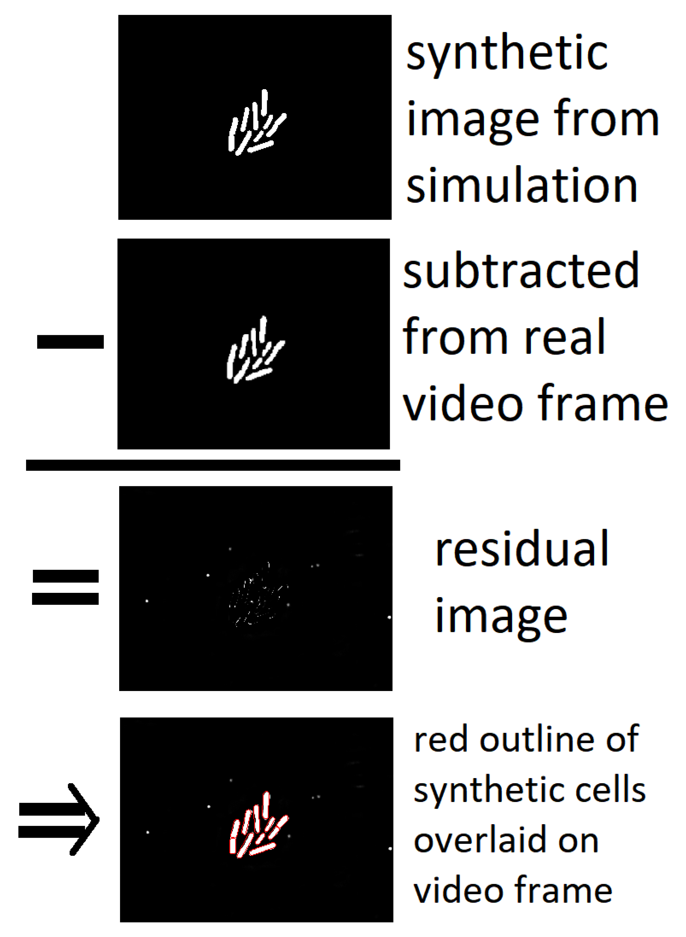
• We maintain a physically-based model of the “universe” so we “know” where every bacterium is at any given moment.
• The model has tight physical constraints over what changes are allowed between frames, so the model effectively “understands” what is possible and what is not.
• These constraints allow us to easily disregard large amounts of noise in the image if they reflect changes that are physically impossible within the constraints of the model.
• Since each and every bacterium has a physical “presence” in our model, it’s highly unlikely to “lose track” of any individual unless even a human would have difficulty tracking the individual (e.g., if it moves off screen or becomes blurred and difficult to distinguish from closely-packed neighbors).

3. Methods

Initialization and Simulation Rules

Our input is preprocessed so that each video frame is binarized into a 0–1 image, using a simple binary threshold. Other methods call this image segmentation, and expend enormous effort to create high-quality segmented images in this prepossessing step (Figure 2). We label the binarized frames of the video from 0 through k, representing times $t_0$ through $t_k$ at equally spaced intervals $\Delta t$. These represent the Universe (the capital U distinguishes the real Universe from simulated universes in our ensemble). Within our simulation, each cell c in the system has a position $x_c\left(t\right)$, orientation ${\theta }_c\left(t\right)$, and length $l_c\left(t\right)$. We simulate the evolution of these variables between two nearby, discrete times t and $t+\delta t$ ($\delta t\ll \Delta t$) by insisting that all state variables are continuous in time: $x_c,l_c,$ and ${\theta }_c$ can each change by some small stochastic amount bounded by $O\left(\delta t\right)$, between t and $t+\delta t$. In addition, each cell c is allowed one “bend” point of angle ${\varphi }_c$ if it is longer than a global constant C. Cells that grow beyond the specified maximum length or bend-constant B are presumed to have split. Each cell furthermore has a small probability of splitting into two daughter cells; this probability can be constant, or depend upon parameters such as its current length. Finally, cells are discouraged from overlapping using a simple Hooke’s law-based repulsion when their borders overlap. No other transitions are allowed.

Since the simulation evolves stochastically, it will diverge from the real Universe. To feasibly track the real Universe we we need to create a relatively large ensemble E of simulated universes in the hopes that some fraction of them will remain close to the real Universe; this also requires that $\Delta t$, the time between video frames, is not too large. The simulation is initialized with an ensemble $E_0$ containing one universe $u_0$ at time 0 which resembles the real Universe in video frame 0. We assume that at each time $t_k$, we start with a relatively small ensemble $E_k$ of simulations that satisfy the following properties: (a) they are all within the observational uncertainty of video frame k; (b) they are numerous enough and dispersed from each other enough to reflect the range of possibilities represented by frame k. Then, the simulation progresses from time $t_k$ to $t_{k+1}=t_k+\Delta t$ as follows: we set time $t=t_k$; each universe u in the ensemble $E_k$ evolves independently of all the others from t to $t+\delta t$ using our stochastic, physics-based rules, duplicating as necessary to represent the range of near-futures at $t+\delta t$. We then set $t:=t+\delta t$ and continue until $t=t_k+\Delta t$.

At this point, the ensemble $E_k\left(t_{k+1}\right)$ will contain many more universes u than it started with at $E_k\left(t_k\right)$. As depicted in Figure 1, for each universe $u\in E_k\left(t_{k+1}\right)$ we generate a synthetic binarized image $I_u$ depicting the state of the simulation for universe $u\left(t_{k+1}\right)$, and compute the residual left after subtracting $I_u$ from the binarized video frame $k+1$. We retain only those universes u from $E_k\left(t_{k+1}\right)$ whose residual from the image subtraction falls below some threshold, subject to the same constraints (a) and (b) listed above.

Due to stochastic noise, even our “best” universes may not be very close to the real Universe. Thus, we attempt to improve these remaining universes by “pulling” them as close to reality as possible (cf. Figure 3). We accomplish this by iterating over each universe and checking whether we can lower its residual cost by perturbing the position, orientation, and size each of its bacteria, iterating this process until each universe converges to a local minimum residual. This tends to produce universes in the new space $E_{k+1}$ of the highest possible quality. One might think that all the simulated universes converge to the same point, which would defeat the goal of maintaining sufficient diversity among our population of universes, but this is not observed, for two reasons: our Hooke’s law repulsion disallows all bacteria to simultaneously move to an ideal position; and each universe may have a different number of bacteria since, if a real bacterium has split into two daughter cells between frames i and $i+1$ and the split is not clear, some universes may choose to model this as one bent bacterium and others may decide a split has occured, and the two cases may equally well fit the observations. This step may require modification for more complex systems.

Because of the design of our simulation, the best-fitting universe at $t_{k+1}$ may not have come from the best-fitting universe at time t. This means that the sequence of best-fitting universes may not form a consistent set representing the evolution of one possible universe. In particular, we have observed that, while following a sequence of best-fitting universes from frame-to-frame, it can sometimes occur that two bacteria at time $t_k$ reunite into one bacterium in frame $t_{k+1}$; this is, of course, impossible in the real world (and therefore never happens in any one of our simulated universes), and visually happens only because the best frame at $t_{k+1}$ did not come from the best-fitting one at time $t_k$. However, every universe at time $t_{k+1}$ came from some universe at $t_k$, so continuity can be constructed by following a universe backwards in time. Accordingly, so as to be able to generate consistent lineage trees, we can construct a single universe that is consistent from the beginning to the end of the video by selecting any universe at the end and tracing it backwards through time to frame 0.

The traceback stage also helps address ambiguity introduced by inconsistent or poor segmentation. Suppose, for example, frame k is properly segmented, k + 1 is over-segmented, and k + 2 is properly segmented. In that case, the “correct” universe—that is, the universe most closely corresponding to reality—will simply fail to be the best universe at k + 2. However, its overall cost at the end of the simulation will be lower than that of any other universe, and thus we can consistently trace back the best-scoring universe even if individual frames were poorly segmented.

The simulation takes the most time when generating new universes and their costs, so runtime complexity is based on the total time the simulation spends creating universes. The runtime complexity may be calculated as follows: let the number of bacteria be N and the runtime complexity of the initial cost function be $O\left(N\right)$. For each frame at time t, we generate about F future universes per bacterium, containing N bacteria per universe. There are K universes in the space S. Thus, the total time for generating universes is $FKN$, and the total runtime complexity is $O\left(FK{N}^2\right)$.

4. Results

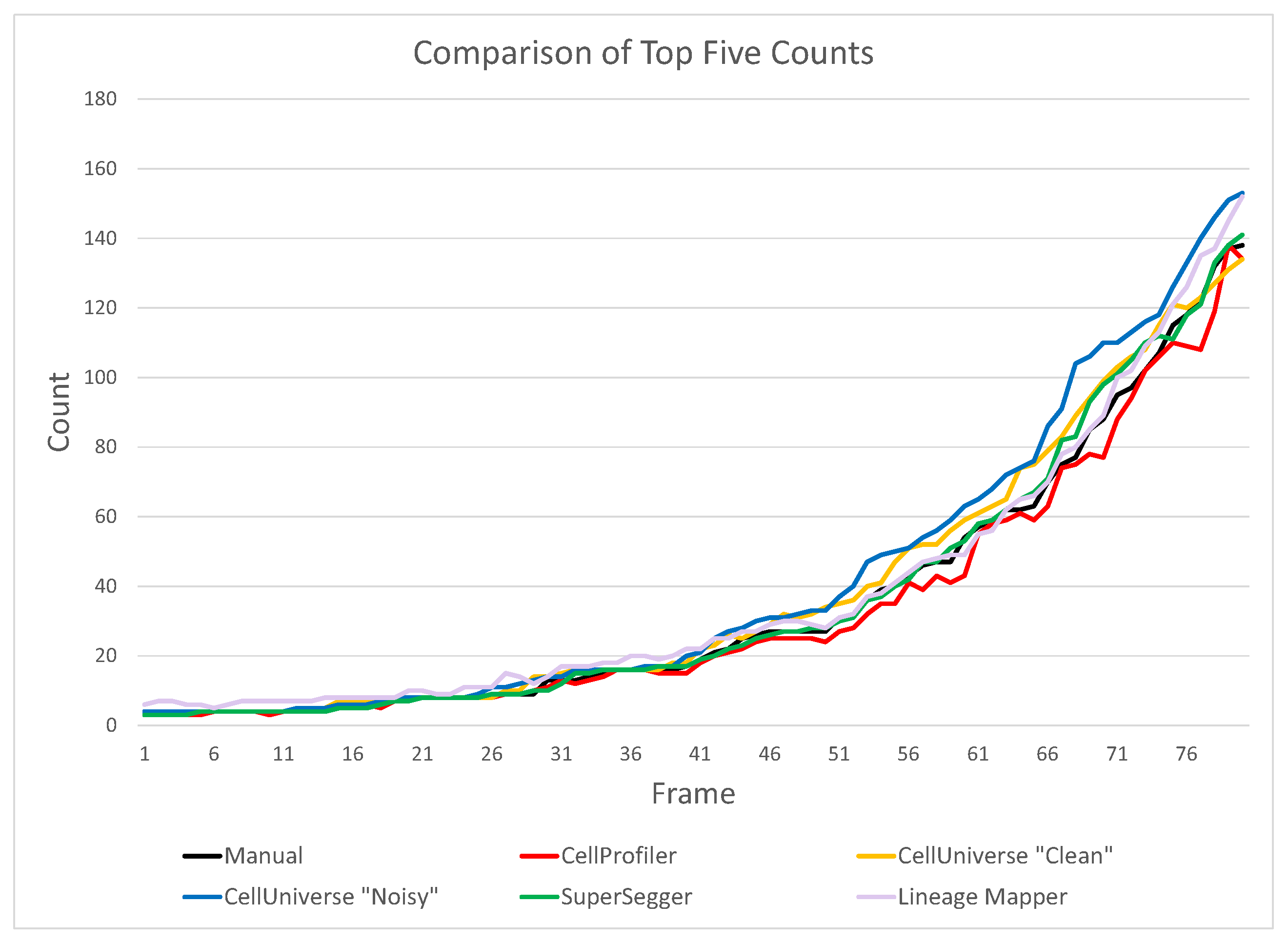
4.1. Bacterial Counting

To evaluate the quality of our simulation’s counts, we ran our simulation on two sets of binarized frames: a “noisy” set and a “clean” set. We used both sets in order to demonstrate that our software is not impeded even by high amounts of noise as depicted at the top of Figure 2. Then, we compared the frame-by-frame bacterial counts produced by our simulation to frame-by-frame bacterial counts we conducted manually on the original video and to the counts produced by a variety of other cell counting and lineage tracking programs, including established programs like CellProfiler [12,13] and more recent programs like SuperSegger [27]. Results are presented in

Table 1. Absolute and relative bacteria count errors for each tested program compared to manual counts, sorted best to worst. A “—” indicates that we were unable to get the program to work on our video. Note: CPU times for all programs other than Cell Universe are only approximate, because each program used its own specific environment (MacOS, Windows, Linux, Matlab, with or without a GUI, etc.). Thus, these tests were run on a highly heterogeneous set of machines with various amounts of RAM, cores, CPU clock speeds, etc.

Program	Err.	%Err.	CPU (s)	Comment
SuperSegger [27]	0.80	2.24	∼2400	10 min $\times 4$ cores on 2.9 GHz Mac
CellProfiler [12,13]	−2.20	−6.17	∼3600	15 min $\times 4$ cores on 3.2 GHz Lenovo G500s i5-3230M
Lineage Mapper [16]	2.84	7.95	∼300	Required enormous effort (days) to tune its parameters
Cell Universe “Clean”	2.85	7.99	9900	20 min $\times 8$ cores on CentOS 2.4 GHz Opteron 6378
TLM-Tracker [28]	−3.55	5.41	∼300	5 min; very sensitive to noise; clean images only.
Cell Universe “Noisy”	5.85	16.40	17,000	35 min $\times 8$ cores on CentOS 2.4 GHz Opteron 6378
ImageJ Reg. Count.	−10.99	−30.80	∼10,000	20 min $\times 8$ cores on CentOS 2.4 GHz Opteron 6378
CellCounter [11]	14.56	40.82	∼1000
Oufti [29]	−29.08	−89.50	∼1000
TrackMate/Fiji [30,31]	37.11	104.30	∼1000
TimeLapseAnal. [32]	—	—	?
LEVER [33]	—	—	?

and depicted in Figure 4.

Our simulation was able to precisely count the number of cells in each frame at least until Frame 66. Between Frames 1–66, any deviations from the manual count were simply because our simulation counted cells as having split into two daughters one frame before they actually did, not because any cells were lost. However, starting in Frame 67 (see Figure 5), problems with the real video began to impact the quality of not only our simulation’s count and the counts of the other techniques, but also our “gold standard” manual count. The real video became blurry as crowding at the center of the colony began to push certain individual bacteria off the camera’s focal plane under the mass of the colony. As a result, neither our simple “clean” nor “noisy” binarizations were entirely able to capture all of the bacteria actually “in” the frame. The combination of blurring and crowding made it difficult for the cost function to measure the difference between reality and the synthetic images created from our simulated universes. However, it is still true that our simulation “knows” some cells are hidden, since they still exist in the simulation even if they are difficult or impossible to discern in the image.

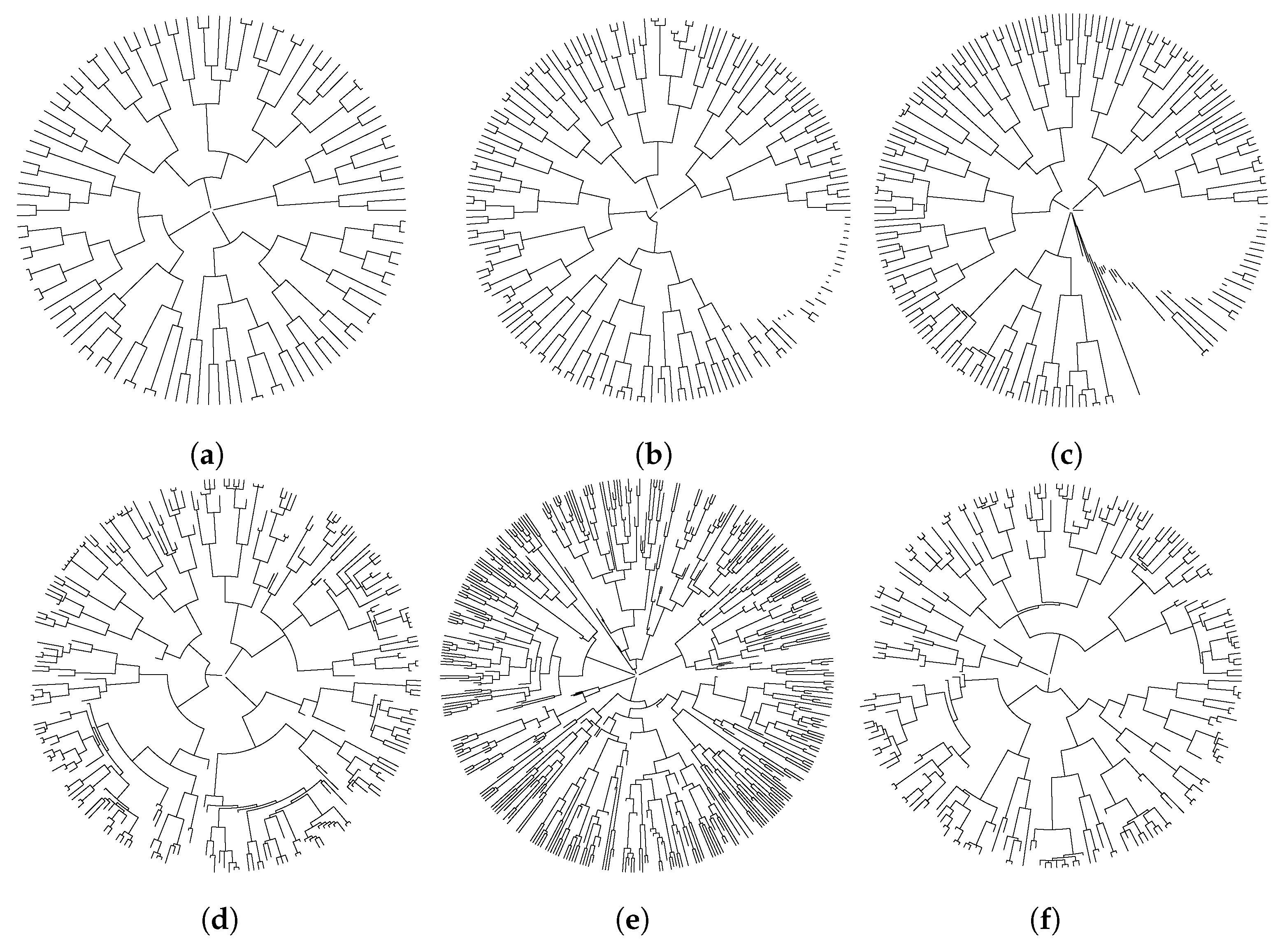
4.2. Cell Lineage Trees

As Table 1 makes evident, Cell Universe is neither the best or the worst at cell counting, although it is significantly better than most, and it was capable of precisely counting up until the point where even a human observer would have begin to have difficulty pinpointing cells. However, simply being able to count individuals without knowing who they are or where they come from is a weak criterion for measuring the success of a tracking algorithm. A stringent, meaningful standard for tracking requires the algorithm to be able to actually track not only the motion of every single individual cell, but also each cell’s entire motion history and family lineage all the way back to the first frame. Cell Universe handily meets this standard, while to our knowledge no other package does.

In the simulation, we give each bacterium a name which is a binary string, and whenever it splits the two daughters inherit the parent’s name with a 0 or 1 appended. For example, a bacterium named ’10’ will split into two children named ’100’ and ’101’. We output the name, position, and orientation of every bacterium in a universe in a corresponding text file. This naming system enables us to construct a lineage tree of all bacteria at the end of the simulation. This tree appears in Figure 6a alongside the best comparison trees from the programs we tested. Observe that our method does not lose any members, tracks every cell that existed at the beginning of the simulation completely until the end of the simulation, and captures binary splits—the only kind of split that is biologically possible. Contrast our lineage tree with the lineage trees produced by the best of the current methods. In (b,c), cells disappear completely from the simulation or appear spontaneously from nowhere, and in (d), some cells divide into more than two daughters, while (e,f) both losses and over-splitting. We think it worth reiterating that by virtue of our reliance on physical rules, our model does not make any of these mistakes. We are thus able to accurately track bacterial lineages even when the bacteria are packed edge-to-edge, a feat that essentially requires a physical understanding of both the scene and of the plausible events that can occur between frames.

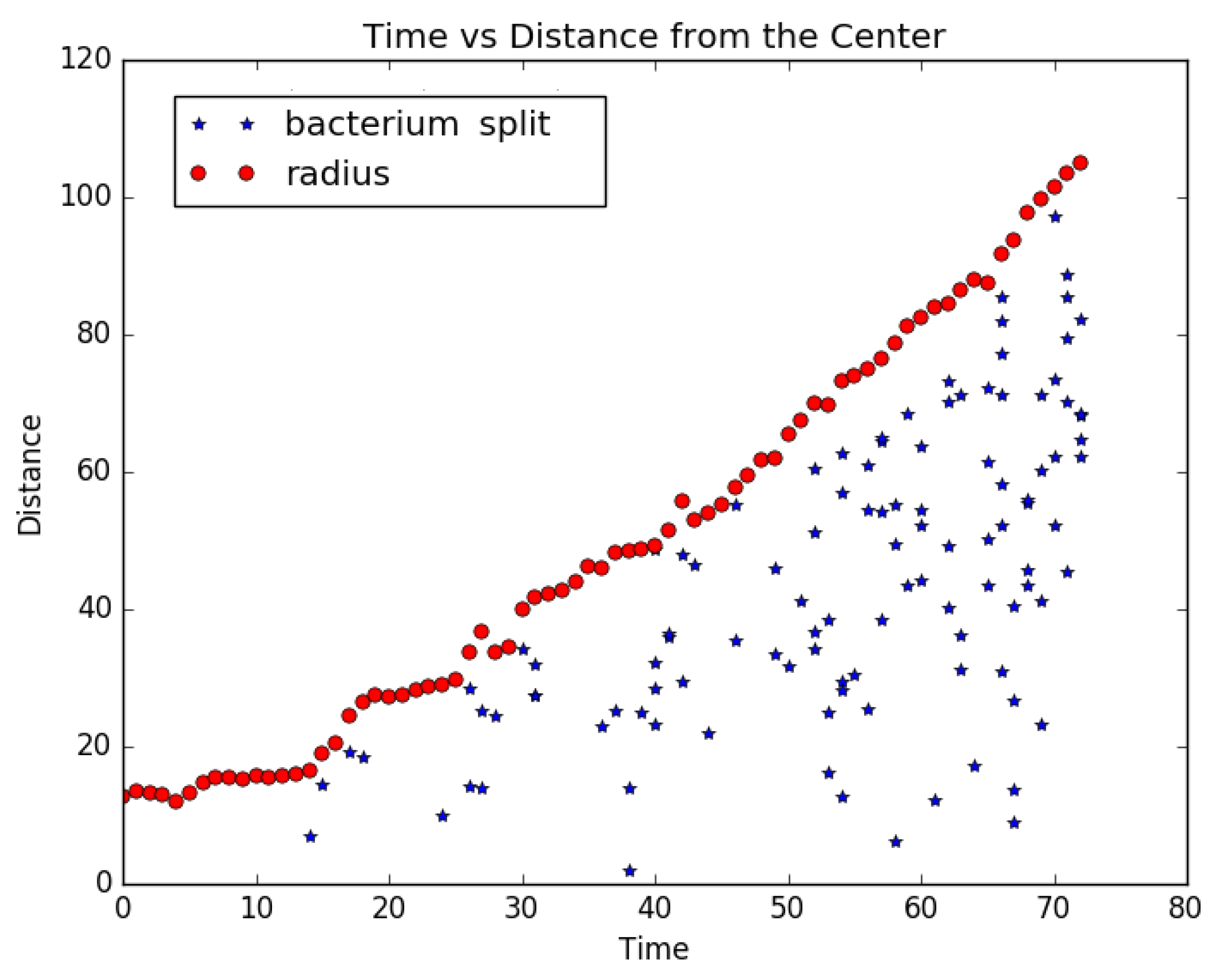
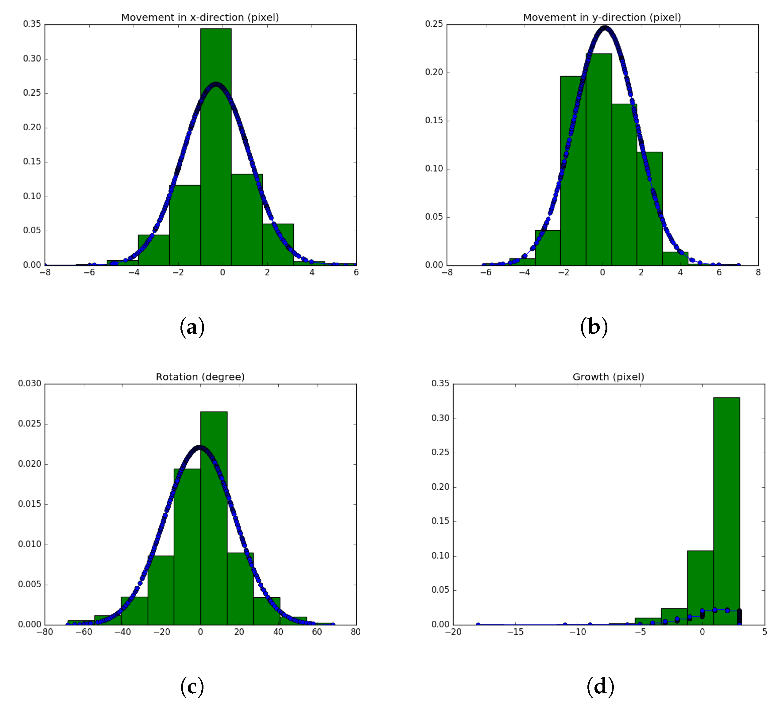
4.3. Precise Motility Measurements

Our detailed knowledge of both the current state and the time-line of historical events allows us to extract information about cell behavior, both individually and in conglomerate, that is otherwise impossible to get. For example, we can make a plot of distance of a bacterium from the center of its colony as a function of time where it splits (Figure 7) and correlate this with which generation a bacterium is in when it splits. Consider Figure 7 beyond frame 70: it is clear that bacteria far from the center of the colony are reproducing before those near the center; furthermore, our linear tree informs us that the bacteria along the periphery of the colony near frame 74 are one full generation ahead of the rest of the colony. Thus, reproduction is consistently occurring faster near the periphery by about 14–17% (since frame 70 contains bacteria in both the 6th and 7th generations). This could be due to resource depletion near the center of the colony, or genetic programming telling the closely-packed cells near the center to “slow down” their reproductive rates, or for some other reason—but the fact that reproduction is occurring faster near the periphery would be difficult to discern otherwise, and certainly warrants further investigation.

The ability to directly measure reproduction rates along family lineages illustrates how our method could conceivably help detect the most aggressively growing individual cells in a cancer tumor. For instance, researchers working on single-cell genomic sequencing of cancer cells [34] could use Cell Universe to accurately identify cell lineages inside a tumor that are reproducing the fastest, and then sequence them to measure correlations between mutations and cancer aggression. This effect would be virtually impossible to detect without reliable tracking of every individual in the colony and the resulting highly-accurate family tree, since without the family tree it would be difficult to impossible to determine each cell’s generation, in turn making it difficult to discern which cell lines are reproducing fastest.

Recall that our simulation model maintains a precise location and orientation of every bacterium. Since our synthetic image is precisely fit to the real image (cf. Figure 1), these positions tend to be extraordinarily precise. For example, since each cell occupies dozens of pixels, the mean location of the cell’s “center” can be determined to sub-pixel accuracy. This allows us to infer detailed statistics on cell motility simply by outputting the positions and orientations of our simulated bacteria, since these are good approximations to that of the real bacteria they represent. Figure 8 plots histograms of per-frame individual bacteria movement, rotation, and growth between video frames. We can see that all the movement and rotation distributions seem to fit a Gaussian curve, while growth in length is more constant at about 2 pixels per frame. We allow slight negative growth not because it is feasible in real life, but because it allows the simulation to correct minor over-estimates in length that can occasionally accumulate over a few consecutive frames.

As evidence of how accurate our per-frame motion measurements are, note that the histogram of motion in the y-direction has a very pronounced skew to the left; motion in the x direction is also skewed left, though is less pronounced. Keep in mind that these distributions are measuring microscopic, sub-pixel sized motions of each and every individual bacterium in each frame, and that these motions are frequently less than a pixel in size between frames. Together, this population average across the motion of individual bacteria suggests that, on average, the colony is moving both downwards and to the left of the image as the video progresses. Interestingly, this conglomerate motion can be easily observed by comparing Figure 2—in which the few bacteria near the beginning of the video are close to the center of the frame—and Figure 5, by which time the entire colony has clearly migrated significantly downwards and to the left in the frame of the camera—exactly as our per-frame distributions suggest. The fact that minuscule, per-frame motion of individual bacteria amounting to only about a pixel per frame, averaged across the population, can easily detect conglomerate motion of the entire colony, attests to the frame-by-frame accuracy of our model colony compared to the real one.

5. Summary, Conclusions & Future Work

We have introduced Cell Universe, which maintains an internal model of the “universe” of cells it is tracking—essentially a complete simulation of the relevant variables of the system being observed—enabling it to “understand” what is happening in the scene, greatly facilitating accuracy and robustness in tracking every single cell that remains clearly visible in the video, without losing track of any individual or its pedigree.

History has shown that learning how to simulate a system can aid making predictions of that system; one could imagine how simulations like those in Cell Universe could aid prediction. For example, we noted that in Figure 8, the per-frame motion in both the x and y directions is skewed slightly towards the negative, allowing us to effectively measure the long-term, large-scale mean motion of the entire colony based on the averaged, short-term and small-scale frame-by-frame motions of its individuals. Thus, the statistical properties of the per-frame motility distributions depicted in Figure 8 have detected a very subtle effect that even we, as the authors, did not notice in the video until we asked ourselves why the distributions were skewed. The next question, of course, is why did the culture grow more quickly towards the bottom left? It could be random, but other possibilities include: was the glass plate tilted? was there a gradient in the density of nutrients on the glass plate? If the latter, then we could potentially derive an empirical relationship between the gradient of nutrient density, and cell movement. Such empirically-derived “laws” could then be used in other contexts to make statistical predictions about cell motility in the large as a function of the environment.

Although Cell Universe offers highly accurate tracking and considerable detail about individual cells, there are several obvious ways in which it could be improved.

• Some systems can capture three-dimensional images whereas Cell Universe currently only handles two dimensions. This will require 3D models of cells to be developed, which adds to the size of the parameter space to be searched. In the case of simply-shaped cells such as bacteria, a model consisting of a cylinder with hemispherical ends would readily extend the current 2D rectangle with semi-circular ends.
• Cells can have more complex shapes than bacteria, and higher resolution images may also display interior structure of the cells. Simulating these aspects may require significantly more parameters that need to be optimized; efficiently dealing with a larger number of optimization parameters per cell could be challenging, though the increasing availability of parallel processing may alleviate some of the cost.
• The speed of Cell Universe could be greatly improved by using less costly algorithms such as simulated annealing to optimize just one universe in place of ensemble simulation.
• Its speed could also be greatly increased by moving from Python to a compiled language such as C++.

References

1. Rundo, L.; Militello, C.; Vitabile, S.; Russo, G.; Sala, E.; Gilardi, M.C. A survey on nature-inspired medical image analysis: A step further in biomedical data integration. Fundam. Inform. 2020, 171, 345–365. [Google Scholar] [CrossRef]
2. Li, K.; Chen, M.; Kanade, T.; Miller, E.D.; Weiss, L.E.; Campbell, P.G. Cell Population Tracking and Lineage Construction with Spatiotemporal Context. Med. Image Anal. 2008, 12, 546–566. [Google Scholar] [CrossRef] [PubMed]
3. Maška, M.; Ulman, V.; Svoboda, D.; Matula, P.; Matula, P.; Ederra, C.; Urbiola, A.; España, T.; Venkatesan, S.; Balak, D.M.; et al. A benchmark for comparison of cell tracking algorithms. Bioinformatics 2014, 30, 1609–1617. [Google Scholar] [CrossRef] [PubMed]
4. Meijering, E.; Dzyubachyk, O.; Smal, I.; van Cappellen, W.A. Tracking in cell and developmental biology. Semin. Cell Dev. Biol. 2009, 20, 894–902. [Google Scholar] [CrossRef] [PubMed]
5. Li, F.; Zhou, X.; Ma, J.; Wong, S.T.C. Multiple nuclei tracking using integer programming for quantitative cancer cell cycle analysis. IEEE Trans. Med. Imaging 2010, 29, 96–105. [Google Scholar]
6. Al-Kofahi, O.; Radke, R.J.; Goderie, S.K.; Shen, Q.; Temple, S.; Roysam, B. Automated cell lineage construction: A rapid method to analyze clonal development established with murine neural progenitor cells. Cell Cycle 2006, 5, 327–335. [Google Scholar] [CrossRef] [PubMed] [Green Version]
7. Gamarra, M.; Zurek, E.; Escalante, H.J.; Hurtado, L.; San-Juan-Vergara, H. Split and merge watershed: A two-step method for cell segmentation in fluorescence microscopy images. Biomed. Signal Process. Control 2019, 53, 101575. [Google Scholar] [CrossRef]
8. Zhang, H.P.; Be’er, A.; Florin, E.-L.; Swinney, H.L. Collective motion and density fluctuations in bacterial colonies. Proc. Natl. Acad. Sci. USA 2010, 107, 13626–13630. [Google Scholar] [CrossRef] [Green Version]
9. Padfield, D.; Rittscher, J.; Roysam, B. Coupled minimum-cost flow cell tracking for high-throughput quantitative analysis. Med. Image Anal. 2011, 15, 650–668. [Google Scholar] [CrossRef]
10. Sacan, A.; Ferhatosmanoglu, H.; Coskun, H. CellTrack: An open-source software for cell tracking and motility analysis. Bioinformatics 2008, 24, 1647–1649. [Google Scholar] [CrossRef] [Green Version]
11. Li, X.; Yang, H.; Huang, H.; Zhu, T. Cellcounter: Novel Open-Source Software for Counting Cell Migration and Invasion In Vitro. BioMed Res. Int. 2014, 2014, e863564. [Google Scholar] [CrossRef] [PubMed]
12. Carpenter, A.E.; Jones, T.R.; Lamprecht, M.R.; Clarke, C.; Kang, I.H.; Friman, O.; Guertin, D.A.; Chang, J.H.; Lindquist, R.A.; Moffat, J.; et al. CellProfiler: Image analysis software for identifying and quantifying cell phenotypes. Genome Biol. 2006, 7, R100. [Google Scholar] [CrossRef] [PubMed] [Green Version]
13. Lamprecht, M.R.; Sabatini, D.M.; Carpenter, A.E. CellProfiler: Free, versatile software for automated biological image analysis. BioTechniques 2007, 42, 71–75. [Google Scholar] [CrossRef] [PubMed] [Green Version]
14. Jaqaman, K.; Loerke, D.; Mettlen, M.; Kuwata, H.; Grinstein, S.; Schmid, S.L.; Danuser, G. Robust single particle tracking in live cell time-lapse sequences. Nat. Methods 2008, 5, 695–702. [Google Scholar] [CrossRef] [PubMed] [Green Version]
15. Kan, A.; Chakravorty, R.; Bailey, J.; Leckie, C.; Markham, J.; Dowling, M. Automated and semi-automated cell tracking: Addressing portability challenges. J. Microsc. 2011, 244, 194–213. [Google Scholar] [CrossRef] [PubMed]
16. Chalfoun, J.; Majurski, M.; Dima, A.; Halter, M.; Bhadriraju, K.; Brady, M. Lineage mapper: A versatile cell and particle tracker. Sci. Rep. 2016, 6, 36984. [Google Scholar] [CrossRef] [Green Version]
17. Zhang, B.; Zimmer, C.; Olivo-Marin, J.C. Tracking fluorescent cells with coupled geometric active contours. In Proceedings of the 2004 2nd IEEE International Symposium on Biomedical Imaging: Nano to Macro, Arlington, VA, USA, 18 April 2004; pp. 476–479. [Google Scholar]
18. Baker, R.M.; Brasch, M.E.; Manning, M.L.; Henderson, J.H. Automated, contour-based tracking and analysis of cell behaviour over long time scales in environments of varying complexity and cell density. J. R. Soc. Interface 2014, 11, 386. [Google Scholar] [CrossRef] [PubMed]
19. Dzyubachyk, O.; Essers, J.; van Cappellen, W.A.; Baldeyron, C.; Inagaki, A.; Niessen, W.J.; Meijering, E. Automated analysis of time-lapse fluorescence microscopy images: From live cell images to intracellular foci. Bioinformatics 2010, 26, 2424–2430. [Google Scholar] [CrossRef] [PubMed] [Green Version]
20. Maška, M.; Danek, O.; Garasa, S.; Rouzaut, A.; Munoz-Barrutia, A.; Ortiz-de Solorzano, C. Segmentation and Shape Tracking of Whole Fluorescent Cells Based on the Chan-Vese Model. IEEE Trans. Med. Imaging 2013, 32, 995–1006. [Google Scholar] [CrossRef]
21. Nath, S.K.; Palaniappan, K.; Bunyak, F. Cell Segmentation Using Coupled Level Sets and Graph-Vertex Coloring. Med. Image Comput. Comput. Assist. Interv. 2006, 9 Pt 1, 101–108. [Google Scholar]
22. Whitaker, J.S.; Hamill, T.M.; Wei, X.; Song, Y.; Toth, Z. Ensemble Data Assimilation with the NCEP Global Forecast System. Mon. Weather. Rev. 2008, 136, 463–482. [Google Scholar] [CrossRef] [Green Version]
23. Wang, Y.; Bellus, M.; Wittmann, C.; Steinheimer, M.; Weidle, F.; Kann, A.; Ivatek-Šahdan, S.; Tian, W.; Ma, X.; Tascu, S.; et al. The Central European limited-area ensemble forecasting system: ALADIN-LAEF. Q. J. R. Meteorol. Soc. 2011, 137, 483–502. [Google Scholar] [CrossRef]
24. Demeritt, D.; Cloke, H.; Pappenberger, F.; Thielen, J.; Bartholmes, J.; Ramos, M. Ensemble predictions and perceptions of risk, uncertainty, and error in flood forecasting. Environ. Hazards 2007, 7, 115–127. [Google Scholar] [CrossRef]
25. Dai, A.; Meehl, G.A.; Washington, W.M.; Wigley, T.M.; Arblaster, J.M. Ensemble simulation of twenty–first century climate changes: Business–as–usual versus CO2 stabilization. Bull. Am. Meteorol. Soc. 2001, 82, 2377–2388. [Google Scholar] [CrossRef] [Green Version]
26. Chenouard, N.; Bloch, I.; Olivo-Marin, J.C. Multiple Hypothesis Tracking for Cluttered Biological Image Sequences. IEEE Trans. Pattern Anal. Mach. Intell. 2013, 35, 2736–3750. [Google Scholar] [CrossRef]
27. Stylianidou, S.; Brennan, C.; Nissen, S.B.; Kuwada, N.J.; Wiggins, P.A. SuperSegger: Robust image segmentation, analysis and lineage tracking of bacterial cells: Robust segmentation and analysis of bacteria. Mol. Microbiol. 2016, 102, 690–700. [Google Scholar] [CrossRef] [Green Version]
28. Klein, J.; Leupold, S.; Biegler, I.; Biedendieck, R.; Münch, R.; Jahn, D. Tlm-tracker: Software for cell segmentation, tracking and lineage analysis in time-lapse microscopy movies. Bioinformatics 2012, 28, 2276–2277. [Google Scholar] [CrossRef] [Green Version]
29. Paintdakhi, A.; Parry, B.; Campos, M.; Irnov, I.; Elf, J.; Surovtsev, I.; Jacobs-Wagner, C. Oufti: An integrated software package for high-accuracy, high-throughput quantitative microscopy analysis. Mol. Microbiol. 2016, 99, 767–777. [Google Scholar] [CrossRef]
30. Schindelin, J.; Arganda-Carreras, I.; Frise, E.; Kaynig, V.; Longair, M.; Pietzsch, T.; Preibisch, S.; Rueden, C.; Saalfeld, S.; Schmid, B.; et al. Fiji: An open-source platform for biological-image analysis. Nat. Methods 2012, 9, 676. [Google Scholar] [CrossRef] [Green Version]
31. Tinevez, J.-Y.; Perry, N.; Schindelin, J.; Hoopes, G.M.; Reynolds, G.D.; Laplantine, E.; Bednarek, S.Y.; Shorte, S.L.; Eliceiri, K.W. TrackMate: An open and extensible platform for single-particle tracking. Methods 2017, 115, 80–90. [Google Scholar] [CrossRef]
32. Huth, J.; Buchholz, M.; Kraus, J.M.; Mølhave, K.; Gradinaru, C.; Wichert, G.v.; Gress, T.M.; Neumann, H.; Kestler, H.A. Timelapseanalyzer: Multi-target analysis for live-cell imaging and time-lapse microscopy. Comput. Methods Programs Biomed. 2011, 104, 227–234. [Google Scholar] [CrossRef] [PubMed]
33. Winter, M.; Mankowski, W.; Wait, E.; Temple, S.; Cohen, A.R. Lever: Software tools for segmentation, tracking and lineaging of proliferating cells. Bioinformatics 2016, 32, 3530–3531. [Google Scholar] [CrossRef] [PubMed] [Green Version]
34. Tsoucas, D.; Yuan, G.-C. Recent progress in single-cell cancer genomics. Curr. Opin. Genet. Dev. 2017, 42, 22–32. [Google Scholar] [CrossRef] [PubMed]
Figure 1. Fitting a synthetic image to the corresponding video frame. We use Frame 26 (cf. Figure 2). (Top) synthetic image derived from the positions, sizes, and orientations of the bacteria in one of the many stochastically simulated “universes”at the time of Frame 26, drawn as a binary image of equal dimensions to the real video image. (Second image) the “clean” image of Figure 2. (Residual image) the pixel-by-pixel difference, in absolute value, between the real and synthetic images; black is zero difference. (Bottom) the outline, drawn in red, of the synthetic bacteria of the top image, overlaid on top of the “clean” video frame of Figure 2.
Algorithms 15 00051 g001
Figure 2. Simple thresholding can result in significant noise as seen in Frame 26 (top right). While Cell Universe has no problem dealing with such levels of noise—even across various choices of threshold—most algorithms we tested against require a much cleaner preprocessed (“segmented”) image such as the one at the bottom right. Video courtesy of YouTube https://www.youtube.com/watch?v=UccyM8QeIeE (accessed on 1 December 2021).
Algorithms 15 00051 g002
Figure 3. Schematic diagram of method: We depict moving from frame 40 to frame 41 of the video, with time t labeled along the horizontal axis. The disk represents a small volume element inside the high-dimensional “phase space” containing all relevant measures of the system being tracked. The green dot in the center of the disk represents “reality” (e.g., positions + orientations of all cells), and the size of the disk represents the extent of observational error (e.g., video resolution). All points inside the disk thus represent plausible measurements of the real system to within observational uncertainty. The black dots are the “ensemble” of simulated universes, all assumed to be within observational uncertainty of the real system. The second, largest disk represents the expansion of the ensemble to many plausible futures—many more universes than we had at frame 40, all of them plausible future trajectories of the system, and now occupying a space much larger than the video uncertainty. Between the 2nd and 3rd disks, we perform a “pulling” operation on all the universes, by performing a preliminary fit of each one to video frame 41, which pulls them all “closer” to the reality depicted in frame 41. However, even after this pulling stage, some members of the ensemble remain implausible—outside the measurement uncertainty of video frame 41. These are discarded, giving the smaller disk at the end of the pulling stage, which is then propagated to frame 41. Finally, if there are too many members of the ensemble that remain at frame 41, we take a final sample of the “best-fitting” members to initialize the process at frame 41.
Algorithms 15 00051 g003
Figure 4. The comparison of the counts returned by the top four methods.
Algorithms 15 00051 g004
Figure 5. Between Frames 67 and 68, our algorithm (as well as all of the other techniques) begins to encounter difficulty tracking cell movements in the center of the colony as cells move off of the focal plane (a,b). Some cells removed by our more aggressive “clean” thresholding (c,d) are visible in our lenient, “noisy” thresholding (e,f).
Algorithms 15 00051 g005
Figure 6. A comparison of six lineage trees. They were generated from the parent-child relationship provided for each cell found in each frame. Gaps in the lineage trees, resulting from cells being temporarily untracked for several frames, were filled in. Time starts at the center of the disk and proceeds outwards. (a) Cell Universe Lineage Tree; (b) SuperSegger Lineage Tree; (c) Lineage Mapper Lineage Tree; (d) CellProfiler Lineage Tree; (e) TrackMate Lineage Tree; (f) TLM-Tracker Lineage Tree.
Algorithms 15 00051 g006
Figure 7. Scatter plot showing how far each bacterium was from the center of the image as a function of the time that it split. Red dots represent whichever bacterium is furthest from the center. Past frame 70 it can be seen that splitting is occurring at the periphery before it does closer to the center, because beyond frame 70 there are 12 splits occuring at 40 pixels or more from the center, and zero occurring closer than 40 pixels. Our detailed lineage tree tells us that the resulting daughter cells are in the 7th generation while those closer to the center are only in the 6th, suggesting bacteria near the periphery are are reproducing faster than those near the center—an observation that would be impossible without a correct, detailed family tree.
Algorithms 15 00051 g007
Figure 8. Distribution of per frame changes in position, orientation, and length, derived from fitting our synthetic universe images to the corresponding actual video frame. We see that the motion in the x and y directions tend to be about 1 pixel in magnitude per frame, while rotation average about 20 degrees and growth about 1–3 pixels per frame. (a) Movement in x-direction (pixels); (b) Movement in y-direction (pixels); (c) Rotation (degrees); (d) Growth (pixels).
Algorithms 15 00051 g008