Clustering with Nature-Inspired Algorithm Based on Territorial Behavior of Predatory Animals

Abstract

Clustering constitutes a well-known problem of division of unlabelled dataset into disjoint groups of data elements. It can be tackled with standard statistical methods but also with metaheuristics, which offer more flexibility and decent performance. The paper studies the application of the clustering algorithm—inspired by the territorial behaviors of predatory animals—named the Predatory Animals Algorithm (or, in short: PAA). Besides the description of the PAA, the results of its experimental evaluation, with regards to the classic k-means algorithm, are provided. It is concluded that the application of newly-created nature-inspired technique brings very promising outcomes. The discussion of obtained results is followed by areas of possible improvements and plans for further research.

1. Introduction

The past few years have brought the increasing role of data science and machine learning as universal research domains allowing to get valuable insights from data coming from a variety of fields. Learning paradigms can be classified as supervised and unsupervised. The supervised learning model assumes the availability of the information on the class membership of each training instance [1]. Unsupervised learning corresponds to the task of extracting useful information from unlabelled data. It does not assume any prior knowledge, and it is usually associated with the problems of clustering and outlier detection [2]. Clustering or cluster analysis corresponds to the task of data division into coherent structures, named clusters, which are grouping similar data elements.

While numerous approaches to clustering based on statistical modeling have already been proposed, the use of metaheuristics has become an alternative strategy. It allows not only to achieve substantial clustering quality but also a possibility of including additional factors, such as the variable number of clusters, multiple objectives, etc. [3,4].

The aim of this paper is to provide a new method of clustering based on natural inspiration. It mimics the territorial behaviors of predatory animals. Unlike most of the existing algorithms, it does not use a centroid-based representation of clustering solutions. At the same time, it focuses on forming natural local clusters without employing traditional evaluation criteria based on internal validation indices. We demonstrate here that the proposed approach can bring high quality of clustering solutions, especially for multidimensional problems, with multiple clusters potentially present in the data.

The paper is organized as follows. The following section is dedicated to the description of related results and methods. It overviews the problem of clustering and nature-inspired techniques used to solve it. In Section 3, the description of the proposed algorithm, in both descriptive and more formal (pseudo-code) way are provided. Section 4 provides the results of numerical experiments aimed at evaluating the performance of the introduced algorithm and comparing it to the standard k-means clustering technique. The paper concludes in Section 5 with final comments and plans for further research.

2. Methodological Background

2.1. Task of Clustering

Let us denote $Y=[y_1,y_2,\dots ,y_M]$ as the dataset under consideration. The task of clustering is equivalent to finding an assignment of data elements $y_1,\dots ,y_M$ to one of the sets (clusters) $C{L}_1,C{L}_2,\dots ,C{L}_C$. This assignment should ascertain that elements designated to the same cluster should be similar to each other.

Typical examples of clustering algorithms include the partitional approach of k-means [5], hierarchical grouping also known as agglomerative clustering [6] and density-based algorithms such as DBSCAN [7], or more recent clustering with density peaks [8].

Clustering quality can be measured with a variety of quantitative indicators. So-called internal validity indices are the ones using only labeled results of clustering, and they measure geometrical properties of clustering structures. Among many indices of this type one can name Davies–Bouldin index [9], Calinski–Harabasz index [10] or Silhouette index [11]. Experimental comparison of these indices can be found in [12,13].

2.2. Nature-Inspired Algorithms in Clustering

Clustering approaches using heuristic optimization typically use centroid-based representation of clustering solution. It means that solution is being represented by cluster centers:

$$x_p=\left[u_1,u_2,\dots ,u_C\right].$$

(1)

The problem of clustering is then presented as the standard continuous optimization task, i.e., to find $x^{\ast }$ which satisfies:

$$f\left(x^{\ast }\right)=\underset{x\in S}{max}f\left(x\right),$$

(2)

where $S\subset R^D$, and $f\left(x\right)$ constitutes solution’s x objective function value.

Broad range of existing nature-inspired metaheuristics have been already used for clustering. It includes Particle Swarm Optimization [14], Krill Herd Algorithm [15], Gravitational Search Algorithm [16] or Social Spider Optimization [17].

The well-known K-means algorithm uses within-cluster variance as an optimization criterion. Using metaheuristics allows us to employ a variety of other indicators. Internal validation indices constitute a natural choice for the objective function in clustering [12]. With this respect, among others, Davies–Bouldin index (e.g., in [9]), Calinski–Harabasz index (e.g., in [18]), were already under investigation. The summary of algorithms and optimization criteria used in metaheuristic clustering can be found in [19].

The algorithm introduced in this paper is not conventional in that respect, as it does not employ internal validation indices for performance evaluation. It also does not limit the shape of the clusters to the spherical ones. It makes the solution being worked-out here attractive for solving real-world clustering problem instances.

3. Proposed Approach

Observing solitary, territorial predators, for example, tigers (Panthera tigris), can yield interesting results concerning the shape of their territories and hunting areas. Female tigers tend to form separate, convex territories around areas densely populated with their prey, which can be intuitively considered a natural example of clustering of prey. Each territory is marked unambiguously by a single female individual by their scent and other marks they left, but should an individual left an area for a time long enough, and those marks will fade, leaving the territory ownerless. In this paper, the approach imitating the behavior of tigers (or other similar solitary, territorial predators such as lynxes) is proposed. The generalization of their behavior is proposed as follows:

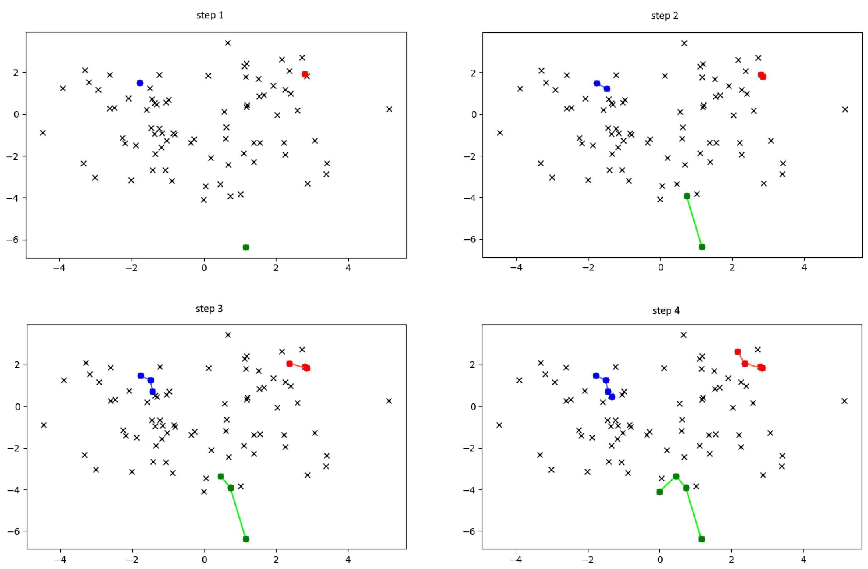
• Clustering is done by the set of (individuals). Each individual has their single position in the given space of instances. This point is always the position of one of the instances and represents the prey the individual is currently hunting. Each individual aims to create a cluster representing their territory.
• Individuals perform jumps between the prey during consecutive turns. On each turn, each individual jumps to a semi-randomly chosen point in the set from the fraction of their closest points, unmarked by other individuals.
• Upon a jump, the individual marks the point they jumped to. From now, it is considered a part of their territory (i.e., their cluster).
• After an individual performs a vast number of jumps far from a point they marked, the traces they left fade, and the location becomes unmarked once again.
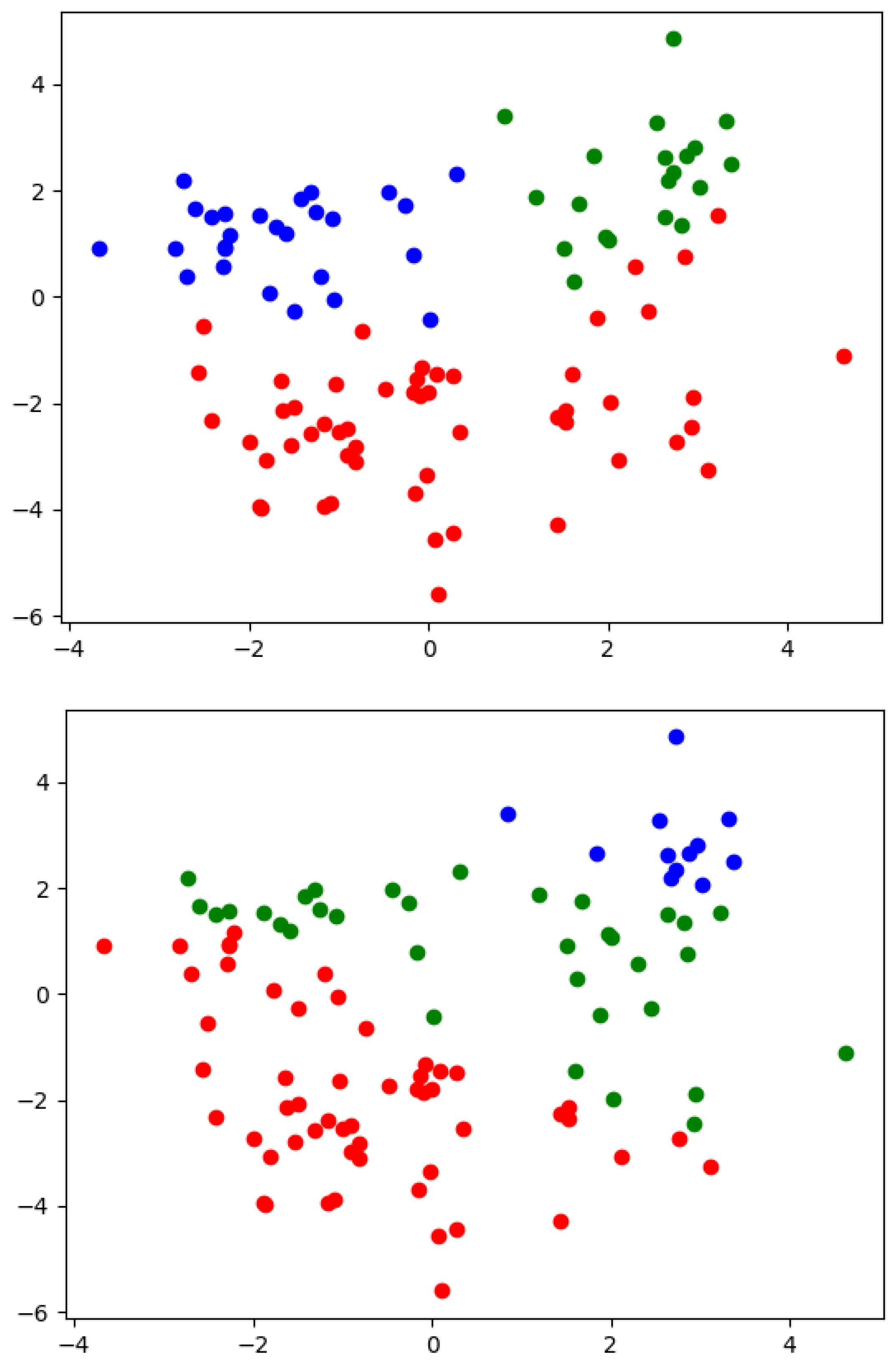
• After all points are marked by individuals, small adjustments are made to simulate fading of areas left behind and making their shape more convex and condensed.

The algorithm generally consists of two phases—the search phase and the correction phase. During the search, individuals create their initial territories (clusters), that are later corrected to simulate the changes that occur in nature. The general pseudo-code of the algorithm can be expressed as in Algorithm 1.

In the formulation of the algorithm the following notation was used:

• $\mathit{dataSet}$ consists of N points, each having their $\mathit{position}$ and $\mathit{cluster}$ (initialized as $\mathit{null}$);
• k is the number of clusters to partition the set into—it has to be predetermined in advance;
• $t_{\mathit{search}}$ is a fraction of the set that will be taken into consideration while determining the next jump of an individual;
• $t_{\mathit{correct}}$ is a is a fraction of the set that will be taken into consideration while determining if it should be corrected;
• b, $M_0$ and S are the parameters of the exponential function used in determining the jump weights;
• $\mathit{alpha}$ is the multiplier factor for correction that simulates the reluctance of changing a set during the correction phase;
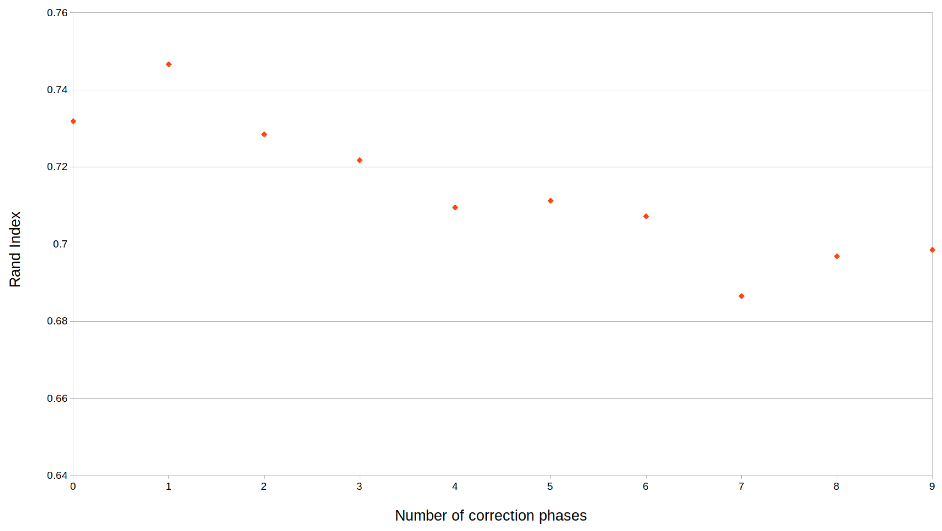
• $\mathit{correctionRuns}$ is the number of times the correction phase is applied;
• F is correction function. Its arguments are $D_{\mathit{mean}}$; the mean distance of points from a given cluster and p, the percentage amount of points from a certain cluster in total points surrounding a point;
• t determines how long does an individual needs to stray from a point it marked for it to become an unmarked point again;
• the algorithm requires the initialization of k; individuals. In this example, their numbers are also the number of their clusters, while the ID of a point is its index.

Algorithm 1 Clustering with Predatory Animals Algorithm.

1: procedurefindClusters($\mathit{dataSet}$, k, $t_{\mathit{correct}}$, $t_{\mathit{search}}$, b, $M_0$, S, $\alpha$, $\mathit{correctionRuns}$, F, T) 2:     $\mathit{MAXTOL}$ ← $\frac{N}{k}\ast T$ 3:     Initialize $I_1,\dots I_k$ as individuals at positions of random points from the set 4:     Set $TTL$ of all points to 0 5:     Set cluster numbers of all points in $\mathit{dataSet}$ as $\mathit{null}$ 6:     for all $I_i\in$ indvididuals do 7:         $\mathit{randomNumber}\leftarrow \mathit{randomIntegerFrom}(0,\mathit{dataSet}.\mathit{size})$ 8:         $I_i.\mathit{position}\leftarrow \mathit{dataSet}\left[\mathit{randomNumber}\right].\mathit{position}$ 9:         $\mathit{dataSet}\left[\mathit{randomNumber}\right].\mathit{cluster}=I_i.\mathit{cluster}\mathit{Id}$ 10:         Remove $\mathit{randomNumber}$ from futher random integer generation in this loop 11:     end for 12:     while there exists at least one point with $\mathit{cluster}=\mathit{null}$ do 13:         for $i\in [1,k]$ do 14:            $\mathit{points}\leftarrow$ set of $t_{\mathit{search}}\ast \mathit{dataSet}.\mathit{size}$ closest points to $I_i$ 15:            $u\leftarrow \frac{\mathit{number}\mathit{Of}(\mathit{points}.\mathit{unmarked})}{t_{\mathit{search}}\ast \mathit{dataSet}.\mathit{size}}$ 16:            for all $P_j\in \mathit{points}$ do 17:                $P_j.\mathit{weight}\leftarrow {(M_0+Su)}^{\frac{1}{b+\mathit{distance}(I_i,P_j)}}$ 18:            end for 19:            $\mathit{point}\mathit{To}\mathit{Jump}\mathit{To}\leftarrow \mathit{randomize}\mathit{With}\mathit{Weights}\left(\mathit{points}\right)$ 20:            $I_i.\mathit{position}\leftarrow \mathit{point}\mathit{To}\mathit{Jump}\mathit{To}.\mathit{position}$ 21:            $\mathit{point}\mathit{To}\mathit{Jump}\mathit{To}.\mathit{cluster}\leftarrow I_i.\mathit{cluster}\mathit{Id}$ 22:         end for 23:         for all $P_j\in$ marked points do 24:            if There exists individual that is closer to $P_j$ than the one that marked it then 25:                $TT{L}_j$ ← $TT{L}_j+1$ 26:                if $TT{L}_j>\mathit{MAXTOL}$ then 27:                    $P_j.\mathit{cluster}$ ← $\mathit{null}$ 28:                end if 29:            end if 30:            Else $TT{L}_j$ ← 0 31:         end for 32:     end while 33:     for $\mathit{iter}=1,2,\dots ,CR$ do 34:         $\mathit{new}\mathit{Cluster}\mathit{Numbers}\leftarrow \mathit{DataSet}.\mathit{cluster}\mathit{Numbers}$ 35:         for all $P_i\in \mathit{DataSet}$ do 36:            $\mathit{points}\leftarrow$ set of $t_{\mathit{correct}}\ast \mathit{DataSet}.\mathit{size}$ closest points to $P_i$ 37:            Initialize table of weights $\mathit{weights}$, its size being the number of clusters 38:            for all $c\in 1,2,\dots ,k$ do 39:                $D_{\mathit{mean}}\leftarrow$ mean distance to all points from cluster c from $\mathit{points}$ 40:                $p\leftarrow$ number of points from cluster c in $\mathit{points}$ divided by size of $\mathit{points}$ 41:                $\mathit{weight}\left[c\right]\leftarrow F(D_{\mathit{mean}},p)$ 42:                if $c\ne P_i.\mathit{cluster}$ then 43:                    $\mathit{weight}\left[c\right]\leftarrow \mathit{weight}\left[c\right]\ast \alpha$ 44:                end if 45:            end for 46:            $\mathit{max}\mathit{Weight}\leftarrow \mathit{index}\mathit{Of}\mathit{Max}\mathit{Element}\left(\mathit{weight}\right)$ 47:            $\mathit{new}\mathit{Cluste}\mathit{Numbers}\left[i\right]\leftarrow \mathit{max}\mathit{Weight}$ 48:         end for 49:         $\mathit{dataSet}.\mathit{cluster}\mathit{Numbers}\leftarrow \mathit{new}\mathit{Cluster}\mathit{Numbers}$ 50:     end for       return $\mathit{dataSet}.\mathit{cluster}\mathit{Numbers}$ 51: end procedure

The first phase (search phase) is performed in turns, during which individuals perform ’jumps’ between unmarked points. An example of few first steps for a simple, small set is shown in the Figure 1. During this phase, the following steps are performed:

• Each individual $I_i$ considers $t_{search}\ast N$ closest points. For each of those points, the individual calculates weight according to the equation $P_j.weight={(M_0+Su)}^{\frac{1}{b+distance(I_i,P_j)}}$, where $P_j$ is the point being evaluated, $M_0,S$ and b are the parameters of the algorithm, and u is the ratio of unmarked points in the evaluated set of points.
• After assigning weights, individuals ‘jump’ to single points they draw with weights they calculated. Those points become their new positions.
• Each marked point is assigned a Time-to-Live value that begins at 0. Each time any of the individuals others than the one that marked the point is the closest individual to that point, the Time-to-Live is incremented. As it reaches $t\frac{N}{k}$, the point becomes unmarked again. Should the individual that marked it become the closest individual, the Time-to-Live value is set to 0 again.
• Individuals perform their jumps in turns until there are no unmarked points. After each turn Time-to-Live values are evaluated for all points in the dataset.

The second phase is focused on slight corrections to the clustered set—it aims to correct points that are surrounded by points from other clusters and not by the points from their own cluster. This is performed in the following way:

• During the correction phase, all points are evaluated separately.
• $t_{correction}\ast N$ nearest points to the evaluated one are considered.
• For each point, for each cluster, values $D_{mean}$ and p are calculated. $D_{mean}$ is the mean normalized distance between the point and points from the currently evaluated cluster and p is the percentage of points from this cluster in the neighbors of the evaluated point.
• Weights determining the cluster to which the given point should be assigned are calculated using correction function $F:{[0,1]}^2\to R$. A cluster with maximum weight is chosen. Function F should be nondecreasing for increasing values of p and not increasing for increasing values of $D_{mean}$. In practice a simple formula $F(p,D_{mean})=D_{mean}/(1.1---p)$ can be used.

It can be seen that the algorithm is based on the natural formation of clusters into disjoint territories. Unlike standard partitional metaheuristic clustering it does not use centroid-based representation and does not rely on internal validation of clusters. The following Section provides an experimental evaluation of this strategy.

4. Experimental Results

During the experimental runs, the proposed algorithm was compared to the standard k-means approach, which is widely used both in research and technical applications.

For the comparison, selected labeled datasets taken from UCI Machine Learning Repository have been used [20]. We have also employed two-dimensional datasets known as s-sets in this experiment [21]. They are characterized by different ratio of clusters overlap. The list of benchmark data used for the experiments can be found in

Table 1. Datasets used in the experiments.

Name	Dimensionality	Number of Clusters	Number of Instances	Source
wine	13	3	178	[22]
glass	10	7	214	[23]
anuran calls	22	10	7195	[24]
gestures	33	5	1000	[25]
libras	90	15	360	[26]
yeast	8	10	1484	[27]
s1	2	15	5000	[21]
s2	2	15	5000	[21]
s3	2	15	5000	[21]
s4	2	15	5000	[21]

.

Both algorithms were executed 100 times. For the newly-introduced PAA we have used the parameters set provided in

Table 2. Parameters of PAA used in the experiments.

Parameter	Value
$t_{search}$	0.05
$t_{correct}$	0.05
$M_0$	2
S	1
$\alpha$	0.8
b	0.001
T	0.3
$F(D_{mean},p)$	$\frac{D_{mean}}{1.1-p}$

.

Table 3. Values of Rand index for PAA and K-means and results of the t-test.

	${\overline{\mathit{R}}}_{\mathbf{PAA}}$	${\overline{\mathit{R}}}_{\mathit{K}}$	Significant Diff.
wine	0.646324	0.658763	0
glass	0.60919	0.506494	0
anuran calls	0.682589	0.471739	+
gestures	0.7235056	0.6380335	+
libras	0.856796	0.8072391	+
yeast	0.621127	0.627	0
s1	0.871717	0.934503	−
s2	0.869067	0.924032	0
s3	0.840887	0.896415	−
s4	0.876354	0.874768	+

provide the results of experiments, with mean of Rand index [28], calculated versus class labels, being used as a performance indicator. The ${\overline{R}}_{\mathit{PAA}}$ represents the average value obtained by the proposed algorithm, while $\overline{R_K}$ the average value obtained using K-Means algorithm. In both cases, the results were taken from 100 repetitions. The last column displays the results of t-test, with significant performance advantage (at $\alpha =0.05$ significance level) of PAA denoted with +, of K-means with −, and not significant difference with 0.

It can be observed that while PAA-based clustering in terms of performance reaches the level of k-means, or it under-performs for simple data division problems (such as s1 or wine) it becomes more competitive for datasets with higher dimensionality. It also offers better performance for clustering instances with overlapping clusters and a more significant number of groups.

Figure 2 illustrates the result of clustering obtained for a dataset consisting of 100 randomly generated points. The positions of the points in the set were created randomly with Gaussian distribution around one point and along three line segments. It has an irregular structure of clusters which are overlapping each other and vary in the density of points. In such a case, the use of PAA is again highly recommended, as it can be observed that a classic algorithm (K-means) yields poor results.

We have also studied the performance of the proposed technique in comparison with the one of the well-know density-based DBSCAN algorithm. In our investigation, we tuned DBSCAN parameters in order to obtain the same number of clusters as for PAA.

Table 4. Values of Rand index for PAA and DBSCAN.

	${\overline{\mathit{R}}}_{\mathbf{PAA}}$	${\overline{\mathit{R}}}_{\mathbf{DBSCAN}}$	DBSCAN Parameters
wine	0.646324	0.408029	$eps=4.7,min\_samples=2$
glass	0.60919	0.59830	$eps=1.35,min\_samples=2$
anuran calls	0.682589	0.749186	$eps=0.33,min\_samples=5$
gestures	0.7235056	0.1193016	$eps=2.9,min\_samples=5$
libras	0.856796	0.74157	$eps=0.9,min\_samples=4$
yeast	0.621127	0.394240	$eps=0.068,min\_samples=4$
s1	0.871717	0.7987187	$eps=2840,min\_samples=20$
s2	0.869067	0.8243575	$eps=2650,min\_samples=20$
s3	0.840887	0.7602578	$eps=2200,min\_samples=20$
s4	0.876354	0.7737063	$eps=1900,min\_samples=20$

contains the results of this experiment. Again, proposed algorithm is superior, in terms of higher Rand index values, for nine out of ten datasets.

It is noticeable that the algorithm’s behavior is controlled by multiple parameters. First of all, it requires the number of clusters k to be provided. As the algorithm has a tendency to considerably reduce sizes of final clusters, providing slightly more clusters than expected as the value of k can be beneficial.

Search threshold $t_{search}$ determines how many of the closets points are considered when creating a new point (making a ’jump’). Increasing this parameter (usually beyond 0.1) makes the algorithm less stable and allows clusters to span along larger distances. Together with $M_0$ this parameter determines the chance for the cluster to form over far-reaching points, thus allowing the algorithm to cross gaps and cluster non-convex points, but also making the shape of the cluster less consistent. Values less or equal to 0.05 of this parameter could be recommended.

Correction threshold $t_{correct}$ determines how many of the closest points are considered when performing correction phase. With this parameter set to 0, the algorithm skips the correction phase. With small values (so that $t_{correct}$*N, N-size of the set is less than 10), it only considers the closest points. Increasing this number beyond $0.01\ast k$ leads to more accurate, yet potentially dangerous correction where certain clusters sizes are unproportionally increased. That is why a value of $0.1$ could be recommended.

After obtaining values of weights used for correction of cluster assignment for each point, the weight of other clusters are multiplied by so called correction reluctance $\alpha$, in order to to reduce chaotic switching points between clusters that are close to each other. Setting this to 0 switches off correction phase, value of 1 makes each cluster treated equally, and raising this value above 1 makes preference for switching cluster to the current one. We have established that the value of $\alpha =0.8$ could be preferable from the performance point of view.

Number of correction runs $CR$ determines how many times correction phase is applied. The larger this number is, the more convex and compact the clusters should be. It is due to removal of small anomalies and points belonging to the clusters outside of them. Setting this value above 1 may lead to smoothing of clusters along planes. During experimental evaluation, optimal number of correction runs $CR$ was estimated to be equal to 1. The illustration for this fact was shown on Figure 3, which provides the average values of Rand index, obtained for 100 runs of the clustering algorithm on the anuran calls dataset.

Finally, each time a new point is chosen randomly to be a part of a cluster, its weight is calculated as ${(M_0+Su)}^{\frac{1}{b+D(I_i,P_j)}}$, where u is number of points where the search occurs divided by search threshold and dataset size. At the same time, D denotes distance between the ith predator and jth point of the considered set. $M_0$ and S scale the base of this exponential function; thus, their increase should lead to less chaotic creation of clusters. As the sum $M_0+Su$ approaches 1, the choice of the next point becomes less influenced by its actual distance to a cluster, up to the limit where it becomes a random choice from uniform distribution. The exponent is the inverse of the distance with b added there to prevent almost-zero values from causing value explosions for small distances. Setting b provides the maximum value the exponent can reach, therefore limiting the value of the whole function. Consequently a values of jump weight exponent bias b, jump weight base $M_0$ and jump weight base scaling S equal to $0.01$, 2 and 1 respectively, could be suggested.

5. Conclusions

The algorithm utilizes an interesting area of animal behavior, focusing on the territorial behaviour of solitary predators rather than the herding behaviour of some species. Although the exact simulation of tigers marking their hunting areas would require including more factors (such as a mating season, reproduction and the differences between the territories of male and female individuals), the first results presented in this paper are either slightly better or at least comparable to those obtained by k-means. In particular, the algorithm seems to work very well for highly dimensional datasets and the ones where many clusters should be identified.

The proposed algorithm can be modified in many various ways, such as studying other weighting functions or considering more factors during the correction phase. The ’territory dissolution’ mechanics of the algorithm can also be changed to a more complex and potentially more effective way of simulating the natural decline of an abandoned territory.

References

1. Sathya, R.; Abraham, A. Comparison of Supervised and Unsupervised Learning Algorithms for Pattern Classification. Int. J. Adv. Res. Artif. Intell. 2013, 2, 34–38. [Google Scholar] [CrossRef] [Green Version]
2. Celebi, M.; Aydin, K. Unsupervised Learning Algorithms; Springer International Publishing: Berlin/Heidelberg, Germany, 2016. [Google Scholar]
3. Srikanth, R.; George, R.; Warsi, N.; Prabhu, D.; Petry, F.; Buckles, B. A variable-length genetic algorithm for clustering and classification. Pattern Recognit. Lett. 1995, 16, 789–800. [Google Scholar] [CrossRef]
4. Bong, C.W.; Mandava, R. Multiobjective clustering with metaheuristic: Current trends and methods in image segmentation. Image Process. IET 2012, 6, 1–10. [Google Scholar] [CrossRef]
5. MacQueen, J. Some methods for classification and analysis of multivariate observations. In Proceedings of the Fifth Berkeley Symposium on Mathematical Statistics and Probability, University of California, Berkeley, CA, USA, 21 June–18 July 1967; pp. 281–297. [Google Scholar]
6. Ward, J.H., Jr. Hierarchical Grouping to Optimize an Objective Function. J. Am. Stat. Assoc. 1963, 58, 236–244. [Google Scholar] [CrossRef]
7. Ester, M.; Kriegel, H.P.; Sander, J.; Xu, X. A Density-Based Algorithm for Discovering Clusters in Large Spatial Databases with Noise; AAAI Press: Menlo Park, CA, USA, 1996; pp. 226–231. [Google Scholar]
8. Rodriguez, A.; Laio, A. Clustering by fast search and find of density peaks. Science 2014, 344, 1492–1496. [Google Scholar] [CrossRef] [PubMed] [Green Version]
9. Kowalski, P.A.; Łukasik, S.; Charytanowicz, M.; Kulczycki, P. Clustering based on the Krill Herd Algorithm with selected validity measures. In Proceedings of the 2016 Federated Conference on Computer Science and Information Systems (FedCSIS), Gdansk, Poland, 11–14 September 2016; pp. 79–87. [Google Scholar]
10. Caliński, T.; Harabasz, J. A dendrite method for cluster analysis. Commun. Stat. 1974, 3, 1–27. [Google Scholar] [CrossRef]
11. Rousseeuw, P.J. Silhouettes: A graphical aid to the interpretation and validation of cluster analysis. J. Comput. Appl. Math. 1987, 20, 53–65. [Google Scholar] [CrossRef] [Green Version]
12. Arbelaitz, O.; Gurrutxaga, I.; Muguerza, J.; Pérez, J.M.; Perona, I. An extensive comparative study of cluster validity indices. Pattern Recognit. 2013, 46, 243–256. [Google Scholar] [CrossRef]
13. Cebeci, Z. Comparison of Internal Validity Indices for Fuzzy Clustering. J. Agric. Inform. 2019, 10, 1–14. [Google Scholar] [CrossRef]
14. Alswaitti, M.; Albughdadi, M.; Isa, N.A.M. Density-based particle swarm optimization algorithm for data clustering. Expert Syst. Appl. 2018, 91, 170–186. [Google Scholar] [CrossRef]
15. Abualigah, L.M.; Khader, A.T.; Hanandeh, E.S. Hybrid Clustering Analysis Using Improved Krill Herd Algorithm. Appl. Intell. 2018, 48, 4047–4071. [Google Scholar] [CrossRef]
16. Han, X.; Quan, L.; Xiong, X.; Almeter, M.; Xiang, J.; Lan, Y. A novel data clustering algorithm based on modified gravitational search algorithm. Eng. Appl. Artif. Intell. 2017, 61, 1–7. [Google Scholar] [CrossRef]
17. Shukla, U.P.; Nanda, S.J. Parallel social spider clustering algorithm for high dimensional datasets. Eng. Appl. Artif. Intell. 2016, 56, 75–90. [Google Scholar] [CrossRef]
18. Łukasik, S.; Kowalski, P.A.; Charytanowicz, M.; Kulczycki, P. Clustering using flower pollination algorithm and Calinski–Harabasz index. In Proceedings of the 2016 IEEE Congress on Evolutionary Computation (CEC), Vancouver, BC, Canada, 24–29 July 2016; pp. 2724–2728. [Google Scholar] [CrossRef]
19. Nanda, S.J.; Panda, G. A survey on nature inspired metaheuristic algorithms for partitional clustering. Swarm Evol. Comput. 2014, 16, 1–18. [Google Scholar] [CrossRef]
20. UCI Machine Learning Repository. Available online: http://archive.ics.uci.edu/ml/ (accessed on 19 February 2021).
21. Fränti, P.; Virmajoki, O. Iterative shrinking method for clustering problems. Pattern Recognit. 2006, 39, 761–775. [Google Scholar] [CrossRef]
22. Aeberhard, S.; Coomans, D.; de Vel, O. Comparative analysis of statistical pattern recognition methods in high dimensional settings. Pattern Recognit. 1994, 27, 1065–1077. [Google Scholar] [CrossRef]
23. Evett, I.W.; Spiehler, E.J. Rule Induction in Forensic Science; Technical Report; Central Research Establishment, Home Office Forensic Science Service: London, UK, 1987.
24. Colonna, J.G.; Cristo, M.; Júnior, M.S.; Nakamura, E.F. An incremental technique for real-time bioacoustic signal segmentation. Expert Syst. Appl. 2015, 42, 7367–7374. [Google Scholar] [CrossRef]
25. Gardner, A.; Kanno, J.; Duncan, C.A.; Selmic, R. Measuring Distance between Unordered Sets of Different Sizes. In Proceedings of the 2014 IEEE Conference on Computer Vision and Pattern Recognition, Columbus, OH, USA, 23–28 June 2014; pp. 137–143. [Google Scholar] [CrossRef] [Green Version]
26. Dias, D.B.; Madeo, R.C.B.; Rocha, T.; Bíscaro, H.H.; Peres, S.M. Hand Movement Recognition for Brazilian Sign Language: A Study Using Distance-Based Neural Networks. In Proceedings of the 2009 International Joint Conference on Neural Networks, Atlanta, GA, USA, 14–19 June 2009; pp. 2355–2362. [Google Scholar]
27. Horton, P.; Nakai, K. A Probabilistic Classification System for Predicting the Cellular Localization Sites of Proteins. In Proceedings of the Fourth International Conference on Computational Biology: Intelligent Systems for Molecular Biology, Washington University, St. Louis, MO, USA, 12–15 June 1996; Volume 4, pp. 109–115. [Google Scholar]
28. Parvin, H.; Alizadeh, H.; Minati, B. Objective criteria for the evaluation of clustering methods. J. Am. Stat. Assoc. 1971, 66, 846–850. [Google Scholar]
Figure 1. Example behaviour of four individuals randomly initialized in a small dataset during first four steps.
Algorithms 15 00043 g001
Figure 2. Comparison of an irregular set clustered by the proposed algorithm (upper figure) and K-means algorithm (bottom figure).
Algorithms 15 00043 g002
Figure 3. The impact of the number of correction runs C R on the performance of the algoritm for anuran calls dataset measured by Rand index.
Algorithms 15 00043 g003