Algorithms for Detecting and Refining the Area of Intangible Continuous Objects for Mobile Wireless Sensor Networks

Abstract

Detecting the intangible continuous object (ICO) is a significant task, especially when the ICO is harmful as a toxic gas. Many studies used steady sensors to sketch the contour and find the area of the ICO. Applying the mobile sensors can further improve the precision of the detected ICO by efficiently adjusting the positions of a subset of the deployed sensors. This paper proposed two methods to figure out the area of the ICO, named Delaunay triangulation with moving sensors (MDT) and convex hull with moving sensors (MCH). First, the proposed methods divide the sensors into ICO-covered and ICO-uncovered sensors. Next, the convex hull algorithm and the Delaunay triangulation geometric architecture are applied to figure out the rough boundary of the ICO. Then, the area of the ICO is further refined by the proposed sensor moving algorithm. Simulation results show that the figured out area sizes of MDT and MCH are 135% and 102% of the actual ICO. The results are better than the planarization algorithms Gabriel Graph (GG) and Delaunay triangulation without moving sensors, that amount to 137% and 145% of the actual ICO. The simulation also evaluates the impact of the sensors’ moving step size to find the compromise between the accuracy of the area and the convergence time of area refinement.

1. Introduction

Wireless sensor networks help us remotely explore unknown fields or dangerous areas such as military areas, hazard environment sensing, and high-temperature industrial monitoring. These tiny devices can monitor the information of their locations and deliver the collected data to the data center via the wireless communication technique. These sensing techniques can reduce the exploring workforce and prevent humans from stepping into dangerous regions.

Numerous studies have focused on detecting the boundary area of the intangible continuous object. Some of these studies organize the deployed sensors into multiple clusters [1,2]. The methods in these studies provide rough boundary results of the continuous object. Their main objective is to track the boundary of a mobile object. Similar proposed studies trace the boundary of a mobile object by using grid architecture [3,4]. These methods divided the deployed region into multiple grids. The sensor in each grid reports whether the continuous object exists or not. The grid size determines the precision of the detected boundary. For refining the detected results, each grid is further divided into multiple smaller grids [4] to improve the detection precision.

In addition, many boundary detection studies used planarization algorithms to figure out the boundary of the continuous object [5,6,7,8,9,10,11]. The sensors in these studies are stationary after being deployed. Their proposed methods treat the sensors as vertices on the planer graph. They create a coarse boundary region to detect the boundary of the continuous objects. The sensors that are covered by the continuous object and close to the boundary line are the inner boundary nodes, and the sensors, which are near the boundary line but uncovered by the continuous object, are outer boundary nodes. All these inner and outer boundary nodes are involved in building the boundary faces. Then, these methods applied the planarization algorithms, such as the Gabriel Graph (GG), Relative Neighborhood Graph (RNG), and k-Localized Delaunay Graph (LDel^k), to create the boundary faces. Considering the communication latency caused by delivering the positions of the sensors, Kundu et al. proposed the farthest-first routing technique to lower the latency [12].

Generally, these planarization algorithms assume that the sensors’ communication range is infinity. The assumption that every sensor can directly communicate with others without considering the physical distance is unrealistic. While considering the limited communication range, the network may determine that the sensors cannot return their positions to the controller. In this scenario, the planarization algorithms will lose their functionality.

Therefore, some studies proposed using mobile sensors to refine the detected boundary of the continuous object [13,14,15]. These methods use a set of mobile sensors traveling within the deploying area to refine the boundary that the stationary sensors have roughly figured out [13,14], or use all sensors to explore all areas of the continuous object. When the continuous object has a long boundary line, these methods may lose their timeliness.

The above methods using stationary sensors to detect the boundary without considering the sensors’ limited communication range are impractical. Therefore, this paper assumes that the sensors have a limited communication range and gives them the mobile ability to refine the boundary precision. The proposed methods applied the convex hull and the Delaunay triangulation methods to estimate the initial area of the continuous object. Next, the sensors’ moving algorithm is adapted to refine the contour of the intangible continuous object (ICO).

2. Related Works

The existing continuous object detection and tracking methods have three classes. The first class comprises the cluster-based methods. Generally, the number of deployed sensors is high. It causes sensors to consume much energy on data propagation. Therefore, this class divides sensors into several small clusters. Every cluster selects a cluster head (CH) to coordinate the sensors’ data communication and collection. Then, the CH aggregates data and delivers them to the sink to reduce the sink’s data receiving requests.

The Dynamic Cluster Structure for Object Detection and Tracking algorithm [1], denoted as DCSODT, proposed by Ji et al., is a cluster-based method. DCSODT adopted a location-based clustering method to trace the continuous object. At first, DCSODT elects the boundary sensors according to the sensing status of the sensors. Next, it verifies the states of the one-hop neighbors of these boundary sensors to determine the cluster. When the continuous object shifts, DCSODT will update the boundary sensors and reform the sensors’ cluster. Although sensors in DCSODT reduce the numerous data transmission to the sink via the cluster structure, they still need to frequently exchange messages with their one-hop neighbors to update the cluster structure.

Chang et al. also proposed a Continuous-Object Detection and Tracking Algorithm, denoted as CODA [2]. CODA dynamically clusters the sensors to detect and trace the continuous object. At first, it divides the sensors into multiple clusters. The CH of each cluster evaluates the locations of the newly joined sensors. Next, CODA models the sensors as the vertices in the geometrical plane and then applies the convex hull algorithm to select the boundary sensors. For reducing the energy consumption of the sensors, the clusters that included any boundary sensors can only send new data to the sink. CODA continuously performs the clustering procedure to update the boundary sensors. The message exchanging during the continuous clustering operation will generate great penalties in communication.

Using the planarization algorithms to detect the boundary area is the role of the second class. The widely used planarization algorithms for constructing the boundary area of the continuous object are Gabriel Graph (GG) [5], Relative Neighborhood Graph (RNG) [6], Delaunay Triangulation [7], k-Localized Delaunay Graph (LDel^k) [8], and Yao Graph (YG) [9]. Generally, the planarization algorithms treat the sensors as vertices on the planer graph. Sun et al. compared the impact of GG, RNG, LDel^k, and YG to analyze the accuracy of detecting the continuous object [16]. They concluded that LDel^k has the best results. They classified the sensors into inner nodes and outer nodes according to whether the sensors detect the event or not. Nodes create a coarse boundary region to predict the boundary of the continuous objects. Usually, these methods focus on building the geometry planer graph and ignore the practical communication range of the sensors.

The third class uses the mobile sensors to adjust the initially deployed positions and then computes a more accurate boundary area. Shu et al. proposed a novel boundary area detection technique named DeGas scheme [13]. DeGas also treats sensors as the vertices of a graph and divides sensors into the inner boundary node (IBN) and the outer boundary node (OBN). Each IBN constructs a link to each one-hop OBN neighbor. This kind of link is named critical edge (CE). The DeGas scheme chooses a CE to explore the connection edges between IBNs and OBNs to build an enclosed area (also called a boundary face) with a mobile car. The proposed method tries to avoid deploying too many redundant sensors.

Shu et al. extended the idea of the DeGas scheme to detect the dangerous area of toxic gases [17]. This method considers the scenario that sensors may be out of function after operating for a while. Each sensor determines itself to be an IBN or an OBN for constructing the Outer Boundary Area (OBA) and Inner Boundary Area (IBA) by checking its one-hop neighbors’ status. The OBA and the IBA are composed of numerous boundary faces, and these faces cover the dangerous area. The area estimation is obtained simply by calculating these irregular boundary faces. This study concluded that creating the boundary faces with the YG graph can yield the highest precision. Ping et al. also proposed a method that uses the planarization algorithms to locate and trace the boundary area of the continuous object with Duty-Cycled WSNs [14]. They used the Kriging algorithm to refine the boundary face area [18]. Zhang et al., proposed a similar novel mechanism for continuous object boundary region detection [15]. To detect a practice boundary, a set of mobile sensors traverses the predicted boundary. It uses a heuristic algorithm like ant colony optimization (ACO) to find the optimal routings for mobile sensors. Experimental results show that the proposed mechanism could get a precise boundary area. Wang et al. used a gas concentration gradient to estimate and track the boundary [19]. A single moving platform with sensors constantly measures the gas concentration [20]. The proposed algorithm controls the motion of a single unmanned underwater vehicle (UUV). As in [19], the initial detection of the cloud boundary and the tracking procedures in this study are obtained according to the calculated toxic substance concentration gradient.

Our previous study proposed an incremental deployment method for detecting the intangible event region, named Incremental Deployment with Gravitational Force (IDGF) [21]. IDGF applied the virtual force model to calculate subsequent sensor positions to track the boundary. Agents are continuously deployed within the region of the intangible events before the coverage area becomes stable. It can reduce the deployed sensors to cover the intangible event’s region. Krzyszto ’n et al., proposed a similar method with five procedures for calculating the optimal values of these parameters [22]. The proposed method also used the virtual force to deploy the sensors.

These methods use stationary sensors to figure out the continuous object. Their precision is limited once the sensors are placed in the deployed area. By involving the mobile sensors, the figured out boundary area of the continuous object can be adjusted further. Thus, this paper adopts mobile sensors to improve precision. The deployed sensors start by building a rough boundary area. Then, the proposed strategy for moving sensors is applied to improve the precision.

3. Proposed Methods

This section gives the main idea of the proposed methods. The first part presents the preliminaries and assumptions. The second part contains the two proposed methods, Delaunay triangulation with moving sensors and convex hull with moving sensors (named MDT and MCH). MDT and MCH use the Delaunay triangulation architecture and the convex hull algorithm to find the rough boundary of the continuous object, respectively. Then they use a sensor moving strategy and a boundary-refining mechanism to improve the precision of the estimated area.

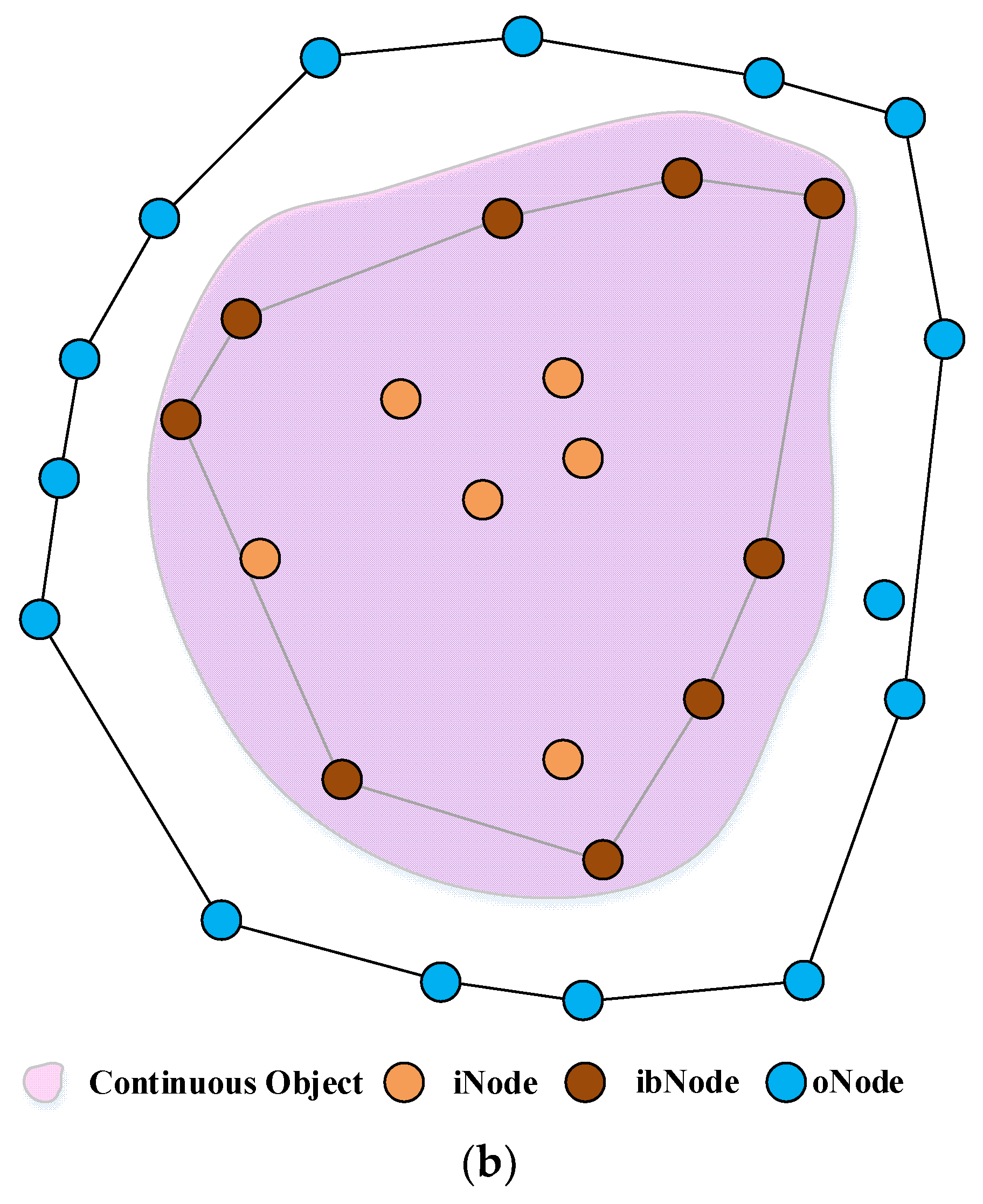
3.1. Preliminaries and Assumptions

In the beginning, sensors are randomly deployed within the region of interest (RoI). These deployed sensors are homogeneous, with the same communication range and sensing range. Each sensor is moveable and can accurately obtain its position. All sensors periodically send their sensed data, identity, and position information to the sink node if the newly sampled data are different from the last ones. The continuous object has an irregular shape. We define that a sensor detects the event if it is within the coverage of the continuous object and its sensed concentration is higher than the threshold.

3.2. The Continuous Object Area Computation

This section shows how the MDT and the MCH figure out the rough area of the continuous object and how to adjust the positions of the boundary sensors to refine the rough area by using the mobile sensors.

3.2.1. Compute the Rough Area of the Continuous Object

All sensors are treated as the vertices (or nodes) on the geometrical plane. All sensors are classified into inner and outer nodes, denoted as the iNode or the oNode. The sensors enclosed within the coverage area of the continuous object are iNodes, and those uncovered are oNodes. In the real world, an iNode is a sensor that detects the concentration of the event higher than a predefined threshold. Here, the notations Ψ_i and Ψ_o are represented as the set of the iNodes and oNodes, respectively.

Next, the MDT applies the Delaunay triangulation to figure out the rough contour of the continuous object. The iNodes, which have any one-hop neighbor in Ψ_o, are retrieved as inner boundary nodes, denoted as ibNodes. Here we use Ψ_i^d′ to represent the set of ibNodes. The one-hop neighbors of iNodes which belong to Ψ_o are outer boundary nodes, denoted as obNodes. We use Ψ_o^d′ as the set of obNodes. Note that a neighbor of a node indicates that its physical distance is shorter than the communication range. All nodes are the vertices of the geographical plane. The Delaunay triangulation of vertices in set Ψ_o^d′∪Ψ_i^d′ is constructed. The summarized areas of these triangulations in the Delaunay triangulation architecture will be the rough area of the continuous object shown in Figure 1. The reason for including the iNodes in set Ψ_i^d′ is to reduce the computation. The iNodes, which are not in Ψ_i^d′, must be in the area enclosed by the sensors in Ψ_i^d′. Therefore, computing the Delaunay triangulation can exclude them to reduce the computation. Involving the oNodes included in Ψ_o^d′ is a way of trying to select the sensors, which are the closest ones to the boundary of the continuous object, for covering all iNodes.

MCH uses the convex- hull algorithm to enclose the continuous object, shown in Figure 2. After finding out the sets Ψ_i and Ψ_o, MCH applies the Graham scan algorithm to obtain the convex hull of the nodes in Ψ_i, shown in Figure 2a. Those nodes, which construct the convex hull of the vertices in Ψ_i, are marked as ibNodes. Let Ψ_i^c′ be the set of these ibNodes. Similarly, the nodes which belong to Ψ_o and are the one-hop neighbors of the vertices in Ψ_i^c′ will be the candidate outer boundary nodes, and we denoted Ψ_o^c as the set of these nodes. The nodes which organize the convex hull of the vertices in Ψ_o^c will be the rough area of the continuous object, shown in Figure 2b. To simplify the presentation, let Ψ_o^c′ be the set of these sensors.

3.2.2. Refine the Enclosed Area with Mobile Sensors

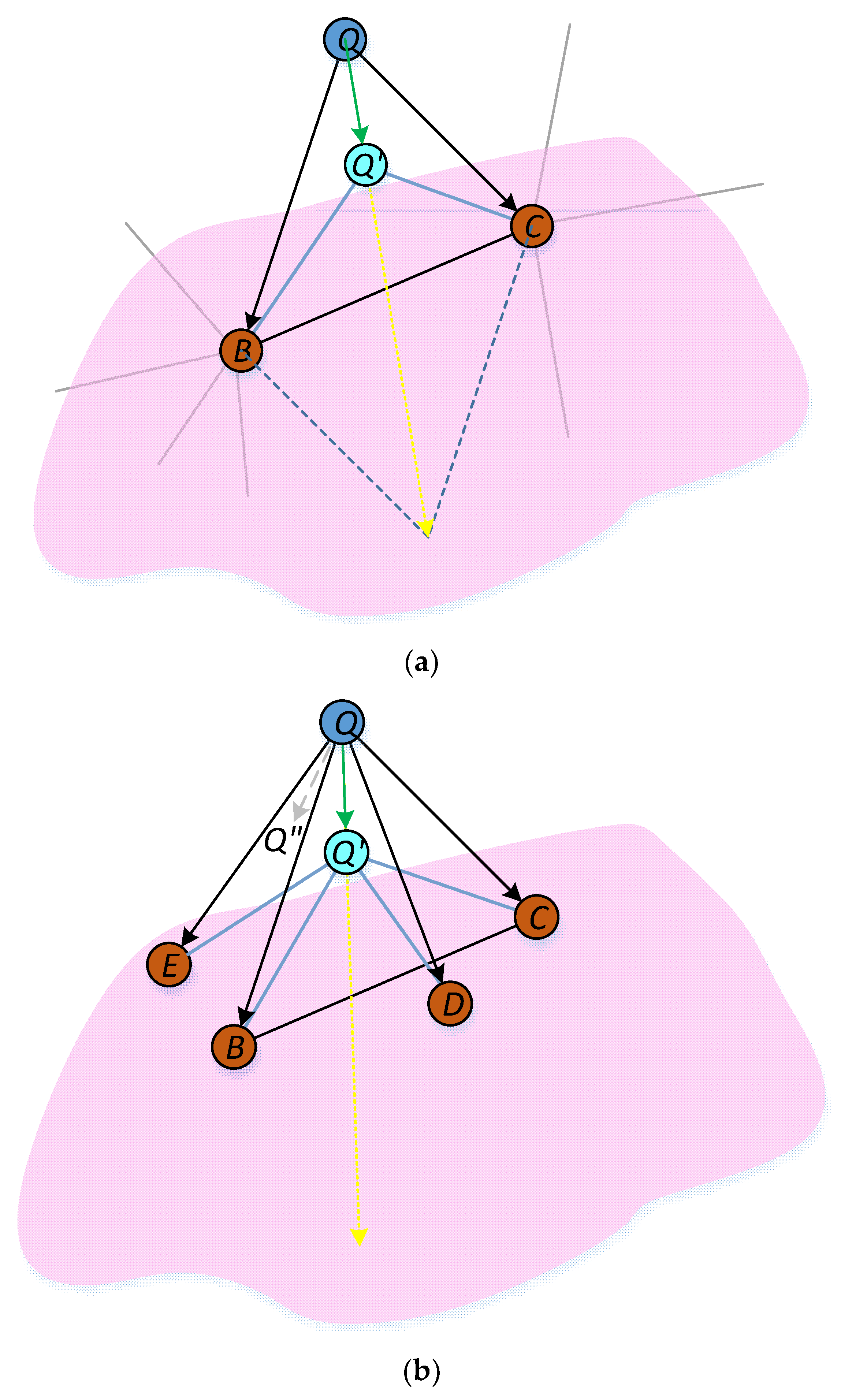
• Determine the moving direction for the sensors

In MDT, the constructed triangulations created by the nodes in sets Ψ_i and Ψ_o must settle on the boundary of the continuous objects. Adjusting the positions of these nodes can refine the bounded area of the continuous object. Let ΔQBC be one of the triangulations constructed by MDT, shown in Figure 3a. The vertex Q is selected to adjust its position because the detecting status of Q is different from the other two vertices, A and B. The moving direction of vertex Q, denoted as D, is computed as the resultant vector of $\stackrel{\rightharpoonup }{QB}$ and $\stackrel{\rightharpoonup }{QC}$. That is, $\stackrel{\rightharpoonup }{D}=\frac{\left(\stackrel{\rightharpoonup }{QB}+\stackrel{\rightharpoonup }{QC}\right)}{|\stackrel{\rightharpoonup }{QB}+\stackrel{\rightharpoonup }{QC|}}$.

In MCH, all the sensors in sets Ψ_i^c′ and Ψ_o^c′ are settled at both sides of the continuous object’s boundary. MCH only selects them to adjust the positions instead of all nodes in Ψ_i^c and Ψ_o^c. This choice can efficiently reduce the number of moving sensors. Considering the moving direction of a sensor Q in Ψ_o^c′, Q firstly collects the position of its one-hop neighbor N_j in Ψ_i^c′ to compute vector $\stackrel{\rightharpoonup }{Q{N}_j}$. Let the number of one-hop neighbors be k. Then, the unit vector of the resultant vector, ${\displaystyle \sum }_{j=1}^k\stackrel{\rightharpoonup }{Q{N}_j}$, will be its moving direction. That is, $\stackrel{\rightharpoonup }{D}=\frac{{{\displaystyle \sum }}_{j=1}^k\stackrel{\rightharpoonup }{Q{N}_j}}{\left|{{\displaystyle \sum }}_{j=1}^k\stackrel{\rightharpoonup }{Q{N}_j}\right|}$, shown in Figure 3b. If sensor Q is in Ψ_i^c′ instead of Ψ_o^c′, the mechanism to determine the moving direction of Q is similar. Q uses its one-hop neighbors in Ψ_i^c′ instead of Ψ_o^c′.

This involves more one-hop neighbors of Q with distinct detected states, which can make the position adjust to the boundary line more efficiently. Suppose that Q only selects two sensors in set Ψ_i^c′ to compute its next target position instead of all one-hop sensors. Without any further information, Q may choose the sensors B and E. This decision makes Q move to location Q”, which is farther away from the boundary than Q’.

• Determine the moving step size of the mobile sensors and location freeze mechanism

Adopting the appropriate moving step size is very important. Using a small moving step size is helpful to improve the precision of the figured area, but it increases the convergence time of the moving operation. Using a large moving step size can shorten the convergence time of the sensors’ moving task, but the sensors will easily cross the boundary of the continuous object. Thus, the maximum value of the moving step size for any sensor Q must be well controlled. Let γ be the moving step size. The maximum value of the moving step size of mobile sensor Q, γ_max, is set to ${\gamma }_{max}=\frac{1}{2}\times \left|\stackrel{\rightharpoonup }{Q{O}_a}+\stackrel{\rightharpoonup }{Q{O}_b}\right|$, where Q_a and Q_b are two of the nodes that determine the moving direction of Q and are closest to Q. Taking half the size of the resultant vector can reduce the probability that the mobile sensor Q crosses the boundary of the continuous object in one movement. Different moving step sizes λ × γ_max|_{0 < λ ≦ 1} will be evaluated in the simulation section. In addition, the proposed algorithms design a moving freeze mechanism to prevent the sensors from overcorrecting their positions. The vertex goes back to its original position and becomes stationary when it detects its status change during its movement. The refinement moving procedure of MDT terminated when all vertices in set Ψ_o^d′∪Ψ_i^d′ become stationary. In MCH, Ψ_i^d′ and Ψ_o^d′ are replaced as Ψ_i^c′ and Ψ_o^c′, respectively. Algorithm 1 shows the completed MDT algorithm.

Algorithm 1. The algorithm of the MDT.

V : Set of the deployed nodes. Ψi : The iNode set. Ψo : The oNode set. Ψid′ : The ibNode set. Ψod′ : The obNode set. Ψ(v): The set that the node v belongs to. The set may be Ψid′ or Ψod′. γ: The moving step size. Es(u): the detecting status of node u. Q.Lock:the lock status of node Q. If its value is true, node Q freezes its moving operation. (QX,QY): the coordinates of node Q. (Q’X,Q’Y): the last coordinates of node Q. For all node u ∊ V Verify the Es(u) and Classify u into sets Ψi and Ψo For all node v ∊Ψi Find the nodes v* which have any one-hop neighbor w ∈ Ψo Put v* to set Ψid′ Put w to set Ψod′ Apply the Delaunay triangulation algorithm on {Ψid′, Ψod′} and put all computed triangles ΔABC into set ΩΔ While (∃ Q# ∈{Ψid′, Ψod′} && Q#.Lock == false){ For all ΔABC ∊ ΩΔ { Get the nodes {A,B,C} of ΔABC If (!(∀{A, B, C}∈Ψid′) or !(∀{A, B, C}∈Ψod′)) { Get Q* ∈{A,B,C} where Ψ(Q*) != Ψ({A,B,C}\Q*) Get {Qa, Qb}∈{A,B,C}, where Ψ(Qa) = Ψ(Qb) If (Q*.Lock == true) Break; Compute the moving direction, $D=\frac{\left(\stackrel{\rightharpoonup }{Q^{*}{Q}^a}+\stackrel{\rightharpoonup }{Q^{*}{Q}^b}\right)}{\left|\stackrel{\rightharpoonup }{Q^{*}{Q}^a}+\stackrel{\rightharpoonup }{Q^{*}{Q}^b}\right|}$ (Q*’X,Q*’Y) ←(Q*X,Q*Y)     //store the current location as the last one (Q*X,Q*Y) ← (Q*X + γ×D.x, Q*Y + γ×D.y)//update the current location   If (the event detection of Q* changes) { Restore the original location, (Q*X,Q*Y)←(Q*’X,Q*’Y) Q*.Lock = true } } } }

• MCH: Refine by updating the boundary nodes.

MCH can refine its enclosed area further. There are still many obNodes near the boundary of the continuous object but not belonging to set Ψ_o^c′ after using mobile sensors to refine the bounded area. For each vertex S | S ∈ Ψ_o^c′, MCH traces every neighboring obNode Q of S to refine the size of the bounded area. For any one-hop neighboring obNode Q of S ∈ Ψ_o^c′, if the detecting status of S and Q are the same, replacing S with Q can reduce the enclosed area size. MCH substitutes Q for S to be the new boundary node.

However, the following cases will not update the MCH’s boundary node. The first case is that the selected S cannot find another neighbor Q within its communication range. There is no other choice for updating the boundary node. The second case is that the selected S has only a one-hop neighbor Q |{Q ∈ Ψ_o^c and Q ∈ Ψ_o^c′}. This neighbor Q has already been the boundary node. So, updating the boundary node is unnecessary. The last one is that the selected S has more than two one-hop neighbors Q|{Q ∈ Ψ_o^c and Q ∉ Ψ_o^c′}, but the area of the created convex hull does not enclose these neighbors. Using them as boundary nodes will increase the bounded area instead of refining it. The Algorithm 2 is the completed MCH algorithm.

Algorithm 2. The algorithm of the MCH.

V : set of the deployed nodes Ψi : the iNode set Ψo : the oNode set Ψic′ : the ibNode set Ψoc′ : the obNode set Ψoc : the one-hop neighbor of the nodes in Ψic′ γ: the moving step size Es(u): the detecting status of node u Q.Lock: the lock status of node Q (QX,QY): the coordinates of node Q (Q’X,Q’Y): the last coordinates of node Q For all node u ∊ V Verify the Es(u) and Classify u into sets Ψi and Ψo Applies the Graham scan algorithm to obtain the convex hull of nodes in Ψi and put the nodes constructing the convex hull as set Ψic′ For all node v ∊Ψic′ Find any one-hop neighbor w ∈ Ψo Put w to set Ψoc Applies the Graham scan algorithm to obtain the convex hull of nodes in Ψoc Put the nodes constructing the convex hull as set Ψoc′   While (∃ Q ∈{Ψic′, Ψoc′} and Q.Lock == false){ If (Q ∈ Ψic′) and (Q has at least one-hop neighbor N ∈ Ψoc′) or (Q ∈ Ψoc′) and(Q has at least one-hop neighbor N ∈ Ψic′) { Compute the moving direction, $D=\frac{{{\displaystyle \sum }}_{j=1}^k\stackrel{\rightharpoonup }{Q{N}_j}}{\left|{{\displaystyle \sum }}_{j=1}^k\stackrel{\rightharpoonup }{Q{N}_j}\right|}$, //k is the number of one-hop neighbors that are in different set from Q (Q’X,Q’Y) ←(QX,QY)   //store the current location as the last one (QX,QY) ← (QX + γ×D.x, QY + γ×D.y)//update the current location If (the event detection of Q* changes) { Restore the original location, (QX,QY)←(Q’X,Q’Y) Q.Lock = true } } } } }   Compute Ae, the enclosed area of the nodes in set Ψoc′ after movement For each S ∊ Ψoc′ { Find the each node Q” ∊ Ψoc, and Q” is a one-hop neighbor of S Replace S with Q” Compute the area A*, the convex hull constructed by the nodes in Ψoc′ If (A* < Ae) Update Ψoc′ = Ψoc − {S} + {Q”} }

4. Simulation Results

This section gives the simulation results. The environmental setup of the simulation is presented in the first part. The numerical results and relative discussion are presented in the next part. The evaluation includes the impacts caused by the number of sensors, the radio range, and the moving step size. The planarization algorithms using stationary sensors are also included for evaluation.

4.1. Environment Setup

The ROI is an 800 m × 800 m area. The total area size of the ICO presented in this paper is 79,601 m². It is an irregular shape without diffusing. The sensors are homogeneous and randomly deployed within the ROI. The estimated numbers of sensors are {100, 300, 500, 700, 900} with communication ranges R set to {60 m, 70 m, 80 m}. The evaluated moving step sizes of the sensors are {γ/2, γ/3, γ/4}, where γ is the maximum moving distance addressed in Section 3.2.2. The simulation results are averaged from 100 random scenarios. This paper defines the terminated threshold, denoted as ϴ. When the distance between the boundary nodes with different detecting statuses is less than ϴ, the proposed algorithm terminates. This paper evaluates the existing methods, the Gabriel Graph (GG) and the Delaunay triangulation with stationary sensors (SDT), and the proposed ones, the Delaunay triangulation with moving sensors (MDT) and the convex-hull with moving sensors (MCH).

The evaluation metrics include the size of the enclosed area, the False-Positive Area (FPA), the True-Negative Area (TNA), the convergence time of the algorithms, the number of moving sensors, and the total number of sensors’ movement. A good algorithm will approximate its enclosed area to that of the continuous object. The FPA is the region included within the enclosed area of an algorithm but not covered by the domain of the continuous object. The TNA is the region covered by the continuous object but not contained within the domain figured by an algorithm. The convergence time evaluates the required time for an algorithm to obtain the output results. The number of moving sensors verifies the number of sensors influenced in boundary adjusting, and the number of sensors’ movements checks the number of issued moving instructions.

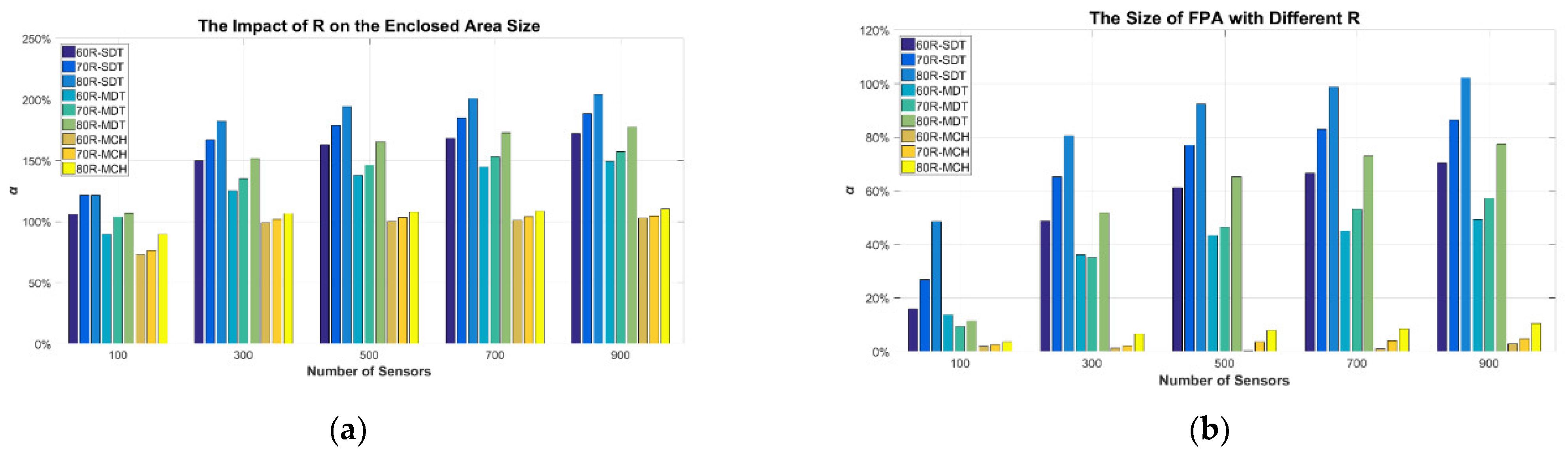
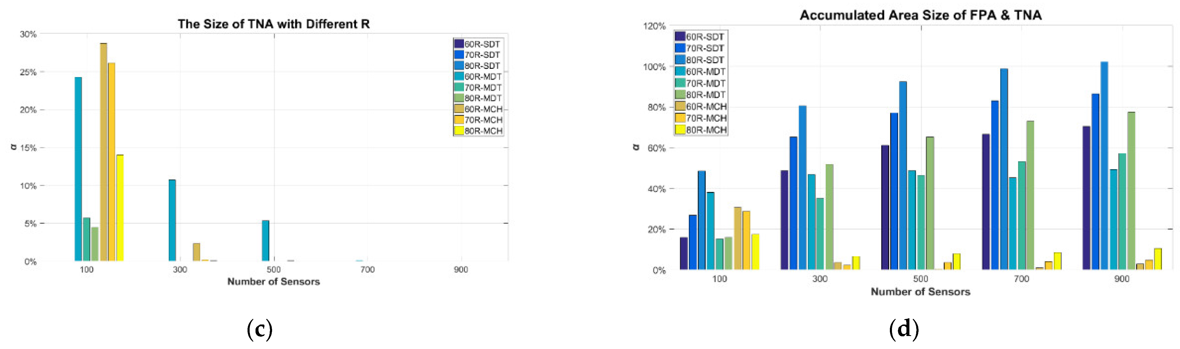
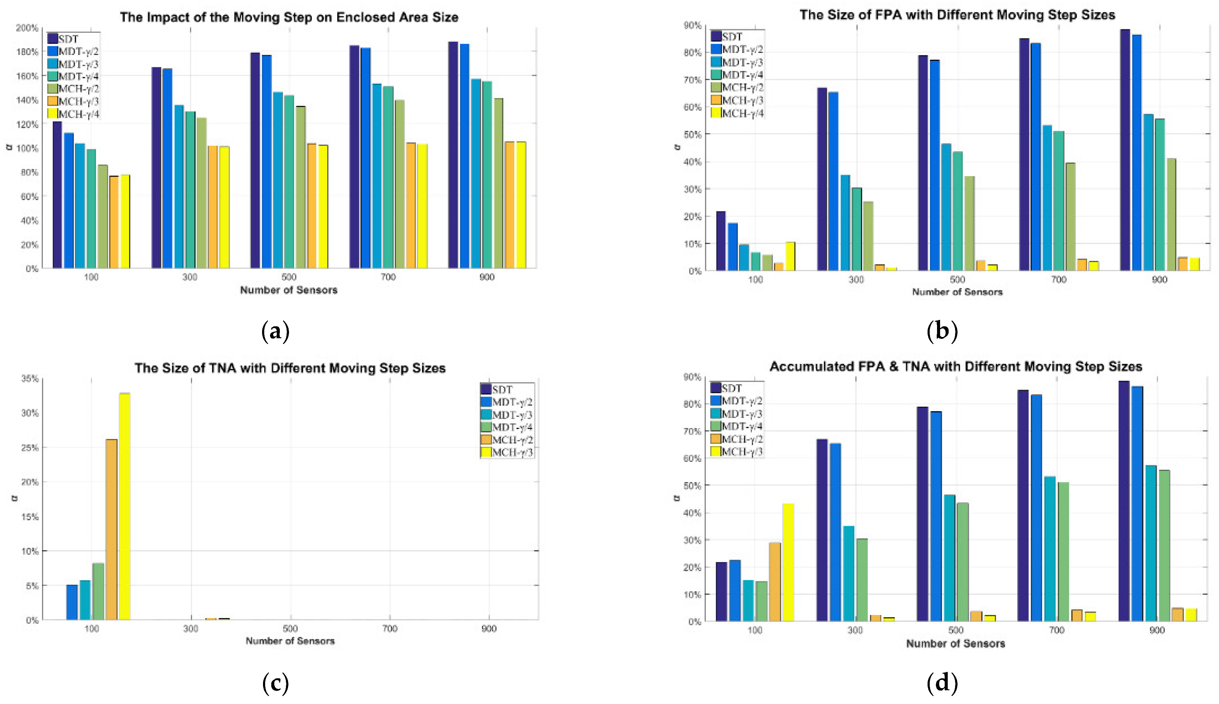
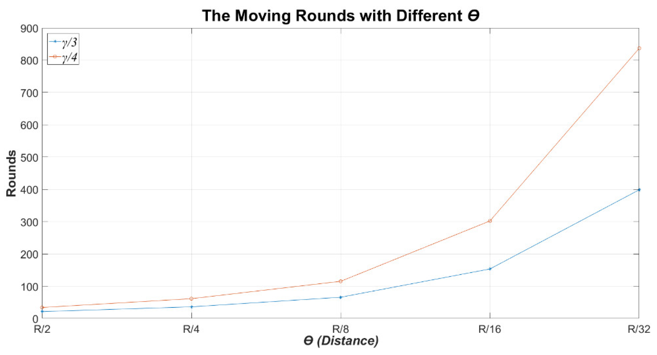
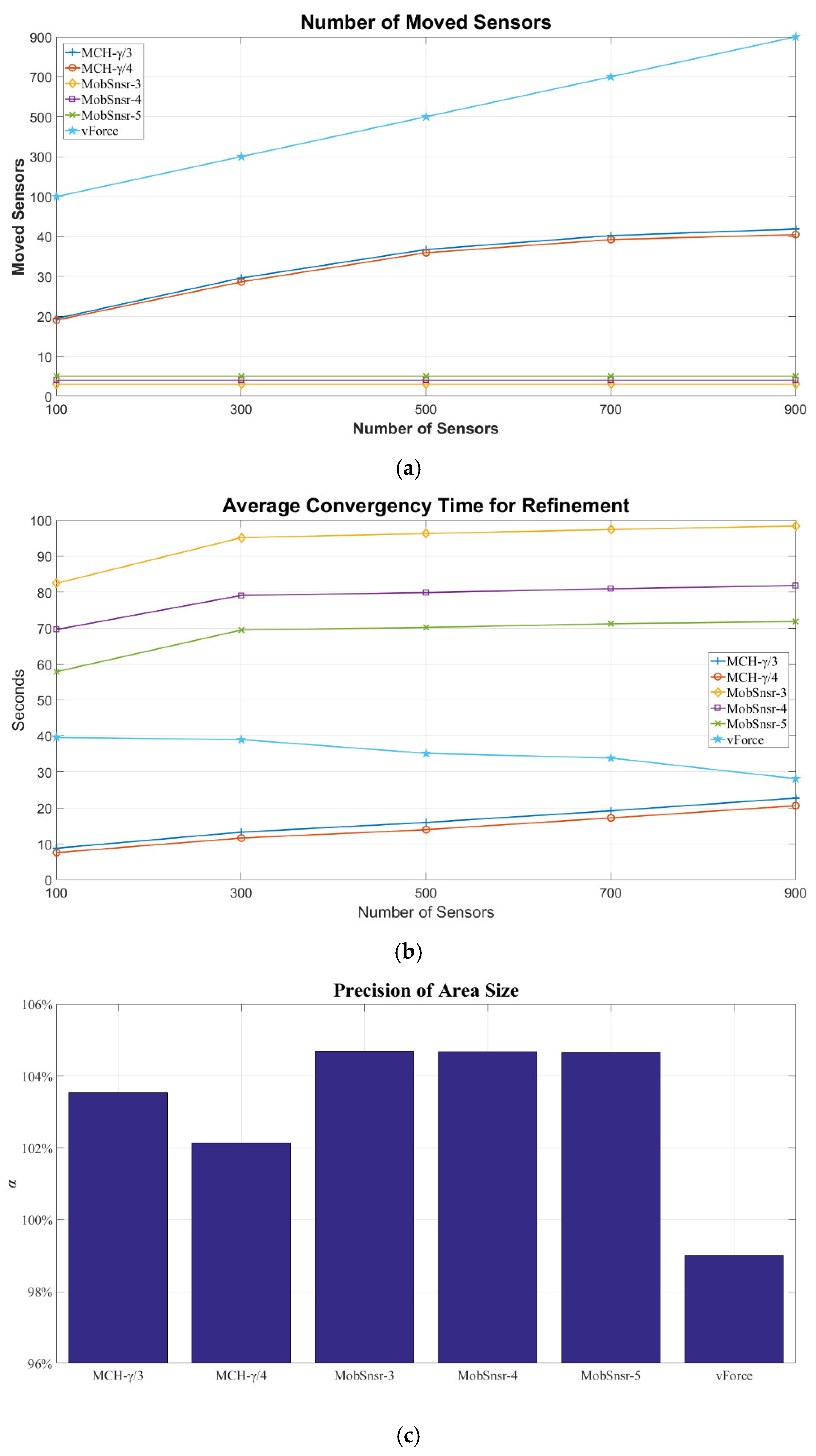
4.2. Numerical Results

Figure 4 shows the comparison of the enclosed area between the existing planarization algorithms (GG and SDT) and the proposed methods (MDT and MCH). In this experiment, the communication range is 70 m, the moving step size is γ/3, and ϴ is R/8. The total area size of the ICO is 79,601 m². In the case of 100 sensors, the deployed sensors are insufficient to cover the whole continuous object. When the number of sensors is more than 300, the enclosed area sizes of GG, SDT, MDT, and MCH are 136.9–160.1%, 144.9–164.5%, 135.1–157.2%, and 104.8%, respectively. GG and SDT bound a larger area than MDT and MCH. MDT is less than SDT (4.4–6.7%) and close to GG (0.1–2.3%). The area size of MCH is very close to the actual size of the continuous object. Its area is less than that of GG and SDT (22.8–32.7% and 29.6–30%, respectively).

Figure 5 evaluates the impact of the communication range R on the size of the enclosed area. This experiment only evaluates SDT, MDT, and MCH, and did not involve GG. This is because GG does not consider the communication range. In this experiment, the moving step size is γ/3, and ϴ is R/8. Let α be the ratio of the area enclosed by an evaluated method over that of the continuous object. An algorithm is said to have high precision if α is close to 100%. In this figure, xxR means that the communication range is xxm. For example, 60R-SDT indicates we apply the SDT algorithm with a communication range of 60 m.

Figure 5a shows that α raises when the number of deployed sensors increases in all methods. The values of α of SDT in 300 sensors are 150%, 167%, and 182% for these three evaluated communication ranges. The values become 172%, 188%, and 204% in 900 sensors. Without adopting the positions of the sensors, the enclosed area size of SDT is 1.5 to 2 times the actual area of the continuous object. For the MDT method, the values of α are about 125%, 135%, and 152% in the case of 300 sensors for the three evaluated communication ranges. The values become 149%, 157%, and 178% in 900 sensors. MDT decreases α by at least 22.6% of the value in SDT for all cases. MCH shows the best results against SDT and MDT. The values of α in 900 sensors are about 103%, 104, and 110% for the three evaluated communication ranges. The results of 100 sensors exhibit different trends because the sensors cannot cover the continuous object completely. Thus, Figure 5b,c shows FPA and TNA for further evaluation.

In Figure 5b, FPA increases as the number of sensors increases. Increasing the number of sensors will introduce more obNodes to enclose the continuous object. So, the enclosed area increases. The increasing trend of FPA gradually becomes moderate as the density of deployed sensors grows. Similarly, increasing the size of R will also include more sensors into the set of obNodes. Because each sensor can cover more area, the size of the total enclosed area grows. In this figure, MDT always has less FPA than SDT in all kinds of R. The FPA of MCH outstands both SDT and MDT, so that its enclosed area sizes are very close to the actual size of the continuous object.

Figure 5c shows the sizes of TNA. SDT almost has no TNA because it encloses more parts of FPA to reduce the possibility of generating TNA. Both MDT and MCH have non-zero sizes of TNA, and the size of TNA efficiently reduces as R grows. Referring to Figure 5b, the payment a using large R is increasing the size of FPA. When the number of sensors is higher than 500, the TNA of MDT is zero. The position adjusting reduces the FPA of MDT. However, part of the experimental scenarios may overcorrect the enclosed area to generate TNA. When the number of sensors increases, this phenomenon disappears.

MCH has more explicitly overcorrection results than the other methods. MCH greedily approximates the actual area of the continuous object to reduce the FPA shown in Figure 5b. This is the main reason why MCH generates more TNA than the other methods. The sizes of the TNA of MDT and MCH are explicitly shown in 100 sensors. This is because the sensors are too few to cover the actual area of the continuous object. Figure 5d shows the accumulated sizes of FPA and TNA. By referring to SDT, MDT can slightly reduce this accumulated size with by adjusting the position of the sensors. The results of MCH are the best indicator that it can fit the actual size of the continuous object more accurately.

Figure 6 evaluates the impact of the moving step size on the enclosed area. In this experiment, the communication range R is 70 m, and ϴ is R/8. Without adjusting the positions of the sensors, SDT has the worst area size shown in Figure 6a. The area size of MDT is close to that of SDT when the moving step size is γ/2. Shortening the moving step size to γ/3 can refine more than 30% of the area size. However, the improvement of the moving step size γ/4 is not as explicit as that of γ/3. The reduced area size is less than 5%. MCH has the best results among all the methods when the moving step size is γ/2. Similarly, the improved area size using moving step size γ/3 is better than that of γ/2 from 31% to 36% when the sensors are more than 300. Compared with the result of γ/3, using γ/4 improves less than 1.5% of the area size.

Figure 6b,c indicates the size of FPA and TNA while applying different moving step sizes. All methods’ FPA and TNA decrease while the moving step size decreases. For the size of FPA, the results of γ/3 and γ/4 are very close. This is also consistent with the results in Figure 6a. The final size of the enclosed area, TNA, and FPA are similar while applying moving step sizes γ/3 and γ/4. The results in 100 sensors do not have the same trend as the others. This is because the sensors cannot fully enclose the continuous object after they adjust their positions. This experiment shows that using a smaller moving step can increase the precision to enclose the actual area of the continuous object. It can be further verified from the accumulated sizes of FPA and TNA shown in Figure 6d.

Figure 7 evaluates the impact of terminating threshold ϴ on the number of moving rounds, and Figure 8 shows the corresponding precision of the proposed MCH algorithm. In this experiment, the communication range R is 70 m, the moving step sizes are {γ/3, γ/4}, and the number of sensors is 900. The round defined in this experiment is that all obNodes and ibNodes need to adjust their positions. It is similar to the times that the algorithm requests to change the topology of the deployed sensors. When the terminating threshold is large, the mobile sensors can quickly step into the stop status shown in Figure 7. However, the enclosed area will have worse precision, as shown in Figure 8. When the terminating threshold is small, shortening the moving step size can improve the precision, but the number of rounds will increase exponentially. The operation rounds by using θ = R/16 is more than twice by using θ = R/8. However, the improved area is 4%. A small terminating threshold makes the sensors frequently adjust their positions within a local region with a minor moving distance, so that the number of rounds grows explicitly. From the results exhibited by these two figures, setting the θ at R/8 seems more suitable for compromising the computation convergence and the area precision.

Figure 9 compares the moving costs spent by the mobile sensors. In this experiment, the communication range R is 70 m, θ is R/8, and the evaluated moving step sizes are {γ/3, γ/4}. This experiment compares the proposed MCH and the method that uses a fixed number of mobile sensors traveling along the selected boundary line to improve the precision of the boundary area [15], denoted as MobSnsr. The sensor’s moving speed is 5 m/s. It is the parameter used by MobSnsr in [15]. The number of mobile sensors of MobSnsr evaluated in this experiment is {3, 4, 5}. The x of MobSnsr-x represents the number of mobile sensors. In addition, the virtual force-based methods proposed in [21,22], are also compared, denoted as vForce.

Figure 9a shows the number of moving sensors used for refining the boundary. The number of mobile sensors in MobSnsr is steady, but the proposed MCH adapts the moving sensors according to the initial deploying topology. Although MCH moves more sensors to refine the boundary, the number of sensors is generally less than 10% of the deployed sensors. The method vForce using the virtual force model makes all deployed sensors continuously adjust their locations to fit the practice area of the continuous object. Therefore, all deployed sensors are moved.

Figure 9b shows the average convergence time in which the mobile sensors finish the boundary-area-refining task. The average time of MobSnsr is about three to five times the time spent by MCH. The vForce method makes all the sensors continuously adjust their positions. Because all the sensors adjust their locations simultaneously, its convergence is still better than that of MobSnsr. A special note is its convergence time decrease as the number of sensors increases. This is because high -density deployed sensors will quickly make the sensors diffuse to the uncovered area. Therefore, the convergence time decreases.

Figure 9c shows the precision of the enclosed area of the experiment in Figure 9. MCH can provide higher accuracy than MobSnsr (1–2.5%). The area precision of the MobSnsr method does not explicitly improve while increasing the number of mobile sensors. However, when the moving step size is γ/4, the area precision is about 102%. The increasing number of mobile sensors is no more than three. The vForce can achieve higher accuracy than MCH and MobSnsr when the sensors are diffused from the covered area of the continuous object. The conclusion is that more sensors are required to adjust their locations and more time is required to make the sensors achieve a stable state.

5. Conclusions

This paper proposed two algorithms to detect the area of intangible continuous objects (ICO), with mobile sensors named Delaunay triangulation with moving sensors (MDT) and convex hull with moving sensors (MCH). First, MDT and MCH classified sensors into ICO-covered ones and ICO-uncovered ones. Then, they applied the Delaunay triangulation and the convex hull techniques on the steady sensors to estimate the rough area of the continuous object, respectively. Next, MDT and MCH used the proposed moving mechanism to adjust the positions of the sensors to refine the enclosed region of the ICO. Simulation results show that MDT can achieve a precision of 135–157% of the actual area of the ICO. MCH can reach 102–145% of that area in ICO. They are better than GG and SDT, which can achieve 137–160% and 145–164% of the actual area of the ICO. The experiments also concluded that moving the step size to γ/4 allows for a precision similar to the one obtained with γ/3. However, the number of termination rounds spent by using γ/4 is about twice as high. Finally, MCH compared the number of moving sensors with the method that uses a steady number of mobile sensors to travel the boundary line for area refinement. Although the proposed MCH moves more sensors than the existing method, the area precision of the proposed MCH can increase 1% to 2.5% by using only one-third to one-fifth of the time spent by the algorithm proposed in [15].

References

1. Ji, X.; Zha, H.; Metzner, J.J.; Kesidis, G. Dynamic cluster structure for object detection and tracking in wireless ad-hoc sensor networks. In Proceedings of the IEEE International Conference on Communications, Paris, France, 20–24 June 2004; pp. 3807–3811. [Google Scholar]
2. Chang, W.; Lin, H.; Cheng, Z. CODA: A Continuous Object Detection and Tracking Algorithm for Wireless Ad Hoc Sensor Networks. In Proceedings of the 5th IEEE Consumer Communications and Networking Conference, Las Vegas, NV, USA, 10–12 January 2008; pp. 168–174. [Google Scholar]
3. Shen, J.; Han, G.; Jiang, J.; Sun, N.; Shu, L. An energy-efficient tracking scheme for continuous objects in duty-cycled wireless sensor networks. In Proceedings of the IEEE International Conference on Consumer Electronics, Taipei, Taiwan, 6–8 June 2015; pp. 150–151. [Google Scholar]
4. Park, B.; Park, S.; Lee, E.; Kim, S.H. Detection and Tracking of Continuous Objects for Flexibility and Reliability in Sensor Networks. In Proceedings of the IEEE International Conference on Communications, Cape Town, South Africa, 23–27 May 2010; pp. 1–6. [Google Scholar]
5. Gabriel, K.R.; Sokal, R.R. A New Statistical Approach to Geographic Variation Analysis. Syst. Biol. 1969, 18, 259–278. [Google Scholar] [CrossRef]
6. Toussaint, G.T. The relative neighbourhood graph of a finite planar set. Pattern Recognit. 1980, 12, 261–268. [Google Scholar] [CrossRef]
7. Rognant, L.; Chassery, J.M.; Goze, S.; Planes, J.G. The Delaunay constrained triangulation: The Delaunay stable algorithms. In Proceedings of the IEEE International Conference on Information Visualization, London, UK, 14–16 July 1999; pp. 147–152. [Google Scholar]
8. Li, X.Y.; Calinescu, G.; Wan, P.J.; Wang, Y. Localized Delaunay triangulation with application in ad hoc wireless networks. IEEE Trans. Parallel Distrib. Syst. 2003, 14, 1035–1047. [Google Scholar]
9. Yao, C.C. On Constructing Minimum Spanning Trees in k-Dimensional Spaces and Related Problems. SIAM J. Comput. 1982, 11, 721–736. [Google Scholar] [CrossRef] [Green Version]
10. Diao, J.; Zhao, D.; Wang, J.; Nguyen, H.M.; Tang, J.; Zhou, Z. Energy-Efficient Boundary Detection of Continuous Objects in IoT Sensing Networks. IEEE Sens. J. 2019, 19, 8303–8316. [Google Scholar] [CrossRef]
11. Zhou, Z.; Zhang, Y.; Yi, X.; Chen, C.; Ping, H. Accurate Boundary Detection and Refinement for Continuous Objects in IoT Sensing Networks. IEEE Commun. Mag. 2019, 57, 93–99. [Google Scholar] [CrossRef]
12. Kundu, S.; Das, N. Event boundary detection and gathering in wireless sensor networks. In Proceedings of the Applications and Innovations in Mobile Computing (AIMoC), Kolkata, India, 12–14 February 2015; pp. 62–67. [Google Scholar]
13. Shu, L.; Mukherjee, M.; Wu, X. Toxic gas boundary area detection in large-scale petrochemical plants with industrial wireless sensor networks. IEEE Commun. Mag. 2016, 54, 22–28. [Google Scholar] [CrossRef]
14. Ping, H.; Zhou, Z.; Rahman, T.; Duan, Y. Localization and tracking of continuous objects boundary area leveraging planar-ization algorithms in duty-cycled wireless sensor networks. In Proceedings of the 43rd Annual Conference of the IEEE Industrial Electronics Society, Beijing, China, 5–8 November 2017; pp. 8476–8481. [Google Scholar]
15. Zhang, Y.; Yi, X.; Zhou, Z.; Shu, L. A Mechanism for Continuous Object Boundary Region Detection and Prediction in Hybrid WSN. In Proceedings of the IEEE 27th International Symposium on Industrial Electronics (ISIE), Cairns, Australia, 13–15 June 2018; pp. 1296–1301. [Google Scholar]
16. Sun, Z.; Wang, H.; Chen, Y.; Shu, L.; Mukherjee, M. Understanding the impact of planarized proximity graphs on toxic gas boundary area detection. In Proceedings of the International Conference on Recent Advances in Signal Processing, Telecom-munications & Computing (SigTelCom), Da Nang, Vietnam, 9–11 January 2017; pp. 109–114. [Google Scholar]
17. Shu, L.; Chen, Y.; Sun, Z.; Tong, F.; Mukherjee, M. Detecting the Dangerous Area of Toxic Gases with Wireless Sensor Networks. IEEE Trans. Emerg. Top. Comput. 2017, 8, 137–147. [Google Scholar] [CrossRef]
18. van Beers, W.C.M.; Kleijnen, J.P.C. Kriging interpolation in simulation: A survey. In Proceedings of the Winter Simulation Conference, Washington, DC, USA, 5–8 December 2004; p. 121. [Google Scholar]
19. Sharma, V.; You, I.; Kumar, R. Energy efficient data dissemination in multi-UAV coordinated wireless sensor networks. Mob. Inf. Syst. 2016, 2016, 8475820. [Google Scholar] [CrossRef] [Green Version]
20. Sharma, V.; Sabatini, R.; Ramasamy, S. UAVs assisted delay optimization in heterogeneous wireless networks. IEEE Commun. Lett. 2016, 20, 2526–2529. [Google Scholar] [CrossRef]
21. Huang, S.-C.; Chang, C.-C.; Chang, H.-Y. Incremental Mobile Sensor Deploying Method for Intangible Event Region De-tection in Wireless Sensor Networks. In Proceedings of the International Conference on Networking and Network Applica-tions (NaNA 2016), Hakodate, Japan, 23–25 July 2016; pp. 360–364. [Google Scholar]
22. Krzysztoń, M.; Niewiadomska-Szynkiewicz, E. Intelligent Mobile Wireless Network for Toxic Gas Cloud Monitoring and Tracking. Sensors 2021, 21, 3625. [Google Scholar] [CrossRef] [PubMed]
Figure 1. The continuous object’s rough area is sketched by MDT. This rough area is figured out by the deployed sensors using their original locations instead of their adjusted locations. The sensors enclosed within the coverage area of the continuous object are iNodes, and those uncovered are oNodes. The nodes in both sets, iNodes and oNodes, closing to the practice boundary of the continuous object, are picked as the vertices in the plane graph to create the Delaunay triangulation.
Algorithms 15 00031 g001
Figure 2. The continuous object’s rough area is sketched by MCH. (a) The sensors included in the set of iNode are involved in finding their convex hull. The sensors used to construct this convex hull are the inner boundary nodes. (b) The sensors included in the set of oNodes are involved in finding their convex hull. The sensors used to construct this convex hull are the outer boundary nodes. The practice boundary of the continuous object is enclosed by the two convex hull polygons built with the sensors in iNode and oNode.
Algorithms 15 00031 g002aAlgorithms 15 00031 g002b
Figure 3. Moving direction of a position-adjusting sensor. (a) The MDT determines a sensor’s moving direction according to the vectors to the other two sensors of the same triangle, which is constructed by the Delaunay triangulation architecture. (b) The MCH determines a sensor’s moving direction according to the vectors of all neighboring sensors that have a different set of convex hull.
Algorithms 15 00031 g003
Figure 4. Compare the Size of the Enclosed Area. This experiment compares the enclosed area of the methods that use mobile sensors and the traditional ones, without mobile sensors. The precision of MDT and MCH is better than that of GG and SDT.
Algorithms 15 00031 g004
Figure 5. The Impact of the Communication Range on the Enclosed Area. (a) The ratio α of the enclosed area sizes. The value of α is the ratio of the area enclosed by an evaluated method over the practice size of the continuous object. An algorithm is said to have high precision if α is close to 100%. (b) The ratio α of FPA in the enclosed area. (c) The ratio α of TNA in the enclosed area. (d) The ratio α of the accumulated FPA and TNA in the enclosed area.
Algorithms 15 00031 g005aAlgorithms 15 00031 g005b
Figure 6. The Impact of Moving Step Sizes on the Enclosed Area (a) The ratio α of the enclosed area sizes. The value of α is the ratio of the area enclosed by an evaluated method over the practice size of the continuous object. An algorithm is said to have high precision if α is close to 100%. (b) The ratio α of the FPA in the enclosed area. (c) The ratio α of the TNA in the enclosed area. (d) The ratio α of the accumulated FPA and TNA in the enclosed area.
Algorithms 15 00031 g006
Figure 7. The number of Moving Rounds with Different Terminated Thresholds. Shortening the moving step size will increase the number of terminating rounds. When the terminating threshold grows, the number of moving rounds decreases. This is because the mobile sensors can quickly step into the stop status.
Algorithms 15 00031 g007
Figure 8. The Precision of the Enclosed Area with Different Terminated Thresholds. When the terminating threshold is small, shortening the moving step size can improve the precision, but the number of moving rounds will increase exponentially (referring to Figure 7). Setting the θ at R/8 is more suitable for compromising the computation convergence and the area precision.
Algorithms 15 00031 g008
Figure 9. The Number of Moving Sensors and the Convergency Time of Refinement. The experiment evaluates the number of moving sensors and the convergency time of the algorithm for moving to the stable state. (a) The number of moving sensors of MCH and the method in [15]. (b) The average convergency time for moving sensors to meet the stable status. (c) The precision of the enclosed area.
Algorithms 15 00031 g009
Publisher’s Note: MDPI stays neutral with regard to jurisdictional claims in published maps and institutional affiliations.