Generalizing the Alpha-Divergences and the Oriented Kullback–Leibler Divergences with Quasi-Arithmetic Means

Abstract

The family of $\alpha$-divergences including the oriented forward and reverse Kullback–Leibler divergences is often used in signal processing, pattern recognition, and machine learning, among others. Choosing a suitable $\alpha$-divergence can either be done beforehand according to some prior knowledge of the application domains or directly learned from data sets. In this work, we generalize the $\alpha$-divergences using a pair of strictly comparable weighted means. Our generalization allows us to obtain in the limit case $\alpha \to 1$ the 1-divergence, which provides a generalization of the forward Kullback–Leibler divergence, and in the limit case $\alpha \to 0$, the 0-divergence, which corresponds to a generalization of the reverse Kullback–Leibler divergence. We then analyze the condition for a pair of weighted quasi-arithmetic means to be strictly comparable and describe the family of quasi-arithmetic $\alpha$-divergences including its subfamily of power homogeneous $\alpha$-divergences. In particular, we study the generalized quasi-arithmetic 1-divergences and 0-divergences and show that these counterpart generalizations of the oriented Kullback–Leibler divergences can be rewritten as equivalent conformal Bregman divergences using strictly monotone embeddings. Finally, we discuss the applications of these novel divergences to k-means clustering by studying the robustness property of the centroids.

1. Introduction

1.1. Statistical Divergences and $\alpha$-Divergences

Consider a measurable space [1] $(\mathcal{X},\mathcal{F})$ where $\mathcal{F}$ denotes a finite $\sigma$-algebra and $\mathcal{X}$ the sample space, and let $\mu$ denotes a positive measure on $(\mathcal{X},\mathcal{F})$, usually chosen as the Lebesgue measure or the counting measure. The notion of statistical dissimilarities [2,3,4] $D(P:Q)$ between two distributions P and Q is at the core of many algorithms in signal processing, pattern recognition, information fusion, data analysis, and machine learning, among others. A dissimilarity may be oriented, i.e., asymmetric: $D(P:Q)\ne D(Q:P)$, where the colon mark “:” between the arguments of the dissimilarities represents the asymmetric property of the division operation. When the arbitrary probability measures P and Q are dominated by a measure $\mu$ (e.g., one can always choose $\mu =\frac{P+Q}{2}$), we consider their Radon–Nikodym (RN) densities $p_{\mu }=\frac{\mathrm{d}P}{\mathrm{d}\mu }$ and $q_{\mu }=\frac{\mathrm{d}Q}{\mathrm{d}\mu }$ with respect to $\mu$, and define $D(P:Q)$ as $D_{\mu }(p_{\mu }:q_{\mu })$. A good dissimilarity measure shall be invariant of the chosen dominating measure so that we can write $D(P:Q)=D_{\mu }(p_{\mu }:q_{\mu })$ [5]. When those statistical dissimilarities are smooth, they are called divergences [6] in information geometry, as they induce a dualistic geometric structure [7].

The most renowned statistical divergence rooted in information theory [8] is the Kullback–Leibler divergence (KLD, also called relative entropy):

$${\mathrm{KL}}_{\mu }(p_{\mu }:q_{\mu }):={\int }_{\mathcal{X}}{p}_{\mu }\left(x\right)log\frac{p_{\mu }\left(x\right)}{q_{\mu }\left(x\right)}\mathrm{d}\mu \left(x\right).$$

(1)

Since the KLD is independent of the reference measure $\mu$, i.e., ${\mathrm{KL}}_{\mu }(p_{\mu }:q_{\mu })={\mathrm{KL}}_{\nu }(p_{\nu }:q_{\nu })$ for $p_{\mu }=\frac{\mathrm{d}P}{\mathrm{d}\mu }$ and $q_{\mu }=\frac{\mathrm{d}Q}{\mathrm{d}\mu }$, and $p_{\nu }=\frac{\mathrm{d}P}{\mathrm{d}\nu }$ and $q_{\nu }=\frac{\mathrm{d}Q}{\mathrm{d}\nu }$ are the RN derivatives with respect to another positive measure $\nu$, we write concisely in the remainder:

$$\mathrm{KL}(p:q)=\int plog\frac{p}{q}\mathrm{d}\mu ,$$

(2)

instead of ${\mathrm{KL}}_{\mu }(p_{\mu }:q_{\mu })$.

The KLD belongs to a parametric family of $\alpha$-divergences [9] $I_{\alpha }(p:q)$ for $\alpha \in \mathbb{R}$:

$$I_{\alpha }(p:q):=\left\{\begin{array}{cc}\frac{1}{\alpha (1-\alpha )}\left(1-\int p^{\alpha }{q}^{1-\alpha }\mathrm{d}\mu \right),\hfill & \alpha \in \mathbb{R}\backslash \{0,1\}\hfill \\ I_1(p:q)=\mathrm{KL}(p:q),\hfill & \alpha =1\hfill \\ I_0(p:q)=\mathrm{KL}(q:p),\hfill & \alpha =0\hfill \end{array}\right.$$

(3)

The $\alpha$-divergences extended to positive densities [10] (not necessarily normalized densities) play a central role in information geometry [6]:

$$I_{\alpha }^{+}(p:q):=\left\{\begin{array}{cc}\frac{1}{\alpha (1-\alpha )}\int \left(\alpha p+(1-\alpha )q-p^{\alpha }{q}^{1-\alpha }\right)\mathrm{d}\mu ,\hfill & \alpha \in \mathbb{R}\backslash \{0,1\}\hfill \\ I_1^{+}(p:q)={\mathrm{KL}}^{+}(p:q),\hfill & \alpha =1\hfill \\ I_0^{+}(p:q)={\mathrm{KL}}^{+}(q:p),\hfill & \alpha =0\hfill \end{array}\right.,$$

(4)

where ${\mathrm{KL}}^{+}$ denotes the Kullback–Leibler divergence extended to positive measures:

$${\mathrm{KL}}^{+}(p:q):=\int \left(plog\frac{p}{q}+q-p\right)\mathrm{d}\mu .$$

(5)

The $\alpha$-divergences are asymmetric for $\alpha \ne \frac{1}{2}$ (i.e., $I_{\alpha }(p:q)\ne I_{\alpha }(q:p)$ for $\alpha \ne \frac{1}{2}$) but exhibit the following reference duality [11]:

$$I_{\alpha }(q:p)=I_{1-\alpha }(p:q)=:I_{\alpha }^{*}(p:q),$$

(6)

where we denoted by $D^{*}(p:q):=D(q:p)$, the reverse divergence for an arbitrary divergence $D(p:q)$ (e.g., $I_{\alpha }^{*}(p:q):=I_{\alpha }(q:p)=I_{1-\alpha }(p:q)$). The $\alpha$-divergences have been extensively used in many applications [12], and the parameter $\alpha$ may not be necessarily fixed beforehand but can also be learned from data sets in applications [13,14]. When $\alpha =\frac{1}{2}$, the $\alpha$-divergence is symmetric and called the squared Hellinger divergence [15]:

$$I_{\frac{1}{2}}(p:q):=4\left(1-\int \sqrt{pq}\mathrm{d}\mu \right)=2\int {(\sqrt{p}-\sqrt{q})}^2\mathrm{d}\mu .$$

(7)

The $\alpha$-divergences belong to the family of Ali–Silvey–Csizár’s f-divergences [16,17] which are defined for a convex function $f\left(u\right)$ satisfying $f\left(1\right)=0$ and strictly convex at 1:

$$I_f(p:q):=\int pf\left(\frac{q}{p}\right)\mathrm{d}\mu .$$

(8)

We have

$$I_{\alpha }(p:q)=I_{f_{\alpha }}(p:q),$$

(9)

with the following class of f-generators:

$$f_{\alpha }\left(u\right):=\left\{\begin{array}{cc}\frac{1}{\alpha (1-\alpha )}(\alpha +(1-\alpha )u-u^{1-\alpha }),\hfill & \alpha \in \alpha \in \mathbb{R}\backslash \{0,1\}\hfill \\ u-1-logu,\hfill & \alpha =1\hfill \\ 1-u+ulogu,\hfill & \alpha =0\hfill \end{array}\right.$$

(10)

In information geometry, $\alpha$-divergences and more generally f-divergences are called invariant divergences [6], since they are provably the only statistical divergences which are invariant under invertible smooth transformations of the sample space. That is, let $Y=m\left(X\right)$ be a smooth invertible transformation and let $\mathcal{Y}=m\left(\mathcal{X}\right)$ denote the transformed sample space. Denote by $p_Y\left(y\right)$ and $p_{Y^{\prime }}\left(y\right)$ the densities with respect to y corresponding to $p_X\left(x\right)$ and $p_{X^{\prime }}\left(x\right)$, respectively. Then, we have $I_f(p_X:p_{X^{\prime }})=I_f(p_Y:p_{Y^{\prime }})$ [18]. The dualistic information-geometric structures induced by these invariant f-divergences between densities of a same parametric family $\{p_{\theta }\left(x\right):\theta \in \mathrm{\Theta }\}$ of statistical models yield the Fisher information metric and the dual $\pm \alpha$-connections for $\alpha =3+2\frac{f^{″}{}^{\prime }\left(1\right)}{f^{″}\left(1\right)}$, see [6] for details. It is customary to rewrite the $\alpha$-divergences in information geometry using rescaled parameter ${\alpha }_A=1-2\alpha$ (i.e., $\alpha =\frac{1-{\alpha }_A}{2}$). Thus, the extended ${\alpha }_A$-divergence in information geometry is defined as follows:

$${\widehat{I}}_{{\alpha }_A}^{+}(p:q)=\left\{\begin{array}{cc}\frac{4}{1-{\alpha }_A^2}\int \left(\frac{1-{\alpha }_A}{2}p+\frac{1+{\alpha }_A}{2}q-p^{\frac{1-{\alpha }_A}{2}}{q}^{\frac{1+{\alpha }_A}{2}}\right)\mathrm{d}\mu ,\hfill & {\alpha }_A\in \mathbb{R}\backslash \{-1,1\}\hfill \\ {\widehat{I}}_1(p:q)={\mathrm{KL}}^{+}(p:q),\hfill & {\alpha }_A=1\hfill \\ {\widehat{I}}_{-1}(p:q)={\mathrm{KL}}^{+}(q:p),\hfill & {\alpha }_A=-1\hfill \end{array}\right.,$$

(11)

and the reference duality is expressed by ${\widehat{I}}_{{\alpha }_A}^{+}(q:p)={\widehat{I}}_{-{\alpha }_A}^{+}(p:q)$.

A statistical divergence $D(·:·)$ when evaluated on densities belonging to a given parametric family $\mathcal{P}=\{p_{\theta }:\theta \in \mathrm{\Theta }\}$ of densities is equivalent to a corresponding contrast function $D_{\mathcal{P}}$ [7]:

$$D_{\mathcal{P}}({\theta }_1:{\theta }_2):=D(p_{{\theta }_1}:p_{{\theta }_2}).$$

(12)

Remark 1.

Although quite confusing, those contrast functions [7] have also been called divergences in the literature [6]. Any smooth parameter divergence $D({\theta }_1:{\theta }_2)$ (contrast function [7]) induces a dualistic structure in information geometry [6]. For example, the KLD on the family $\mathrm{\Delta }$ of probability mass functions defined on a finite alphabet $\mathcal{X}$ is equivalent to a Bregman divergence, and thus induces a dually flat space [6]. More generally, the ${\alpha }_A$-divergences on the probability simplex $\mathrm{\Delta }$ induce the ${\alpha }_A$-geometry in information geometry [6].

We refer the reader to [3] for a richly annotated bibliography of many common statistical divergences investigated in signal processing and statistics. Building and studying novel statistical/parameter divergences from first principles is an active research area. For example, Li [19,20] recently introduced some new divergence functionals based on the framework of transport information geometry [21], which considers information entropy functionals in Wasserstein spaces. Li defined (i) the transport information Hessian distances [20] between univariate densities supported on a compact, which are symmetric distances satisfying the triangle inequality, and obtained the counterpart of the Hellinger distance on the $L^2$-Wasserstein space by choosing the Shannon information entropy, and (ii) asymmetric transport Bregman divergences (including the transport Kullback–Leibler divergence) between densities defined on a multivariate compact smooth support in [19].

The $\alpha$-divergences are widely used in information sciences, see [22,23,24,25,26,27] just to cite a few applications. The singly parametric $\alpha$-divergences have also been generalized to biparametric families of divergences such as the $(\alpha ,\beta )$-divergences [6] or the $\alpha \beta$-divergences [28].

In this work, based on the observation that the term $\alpha p+(1-\alpha )q-p^{\alpha }{q}^{1-\alpha }$ in the extended $I_{\alpha }^{+}(p:q)$ divergence for $\alpha \in (0,1)$ of Equation (4) is a difference between a weighted arithmetic mean $A_{1-\alpha }(p,q):=\alpha p+(1-\alpha )q$ and a weighted geometric mean $G_{1-\alpha }(p,q):=p^{\alpha }{q}^{1-\alpha }$, we investigate a generalization of $\alpha$-divergences with respect to a generic pair of strictly comparable weighted means [29]. In particular, we consider the class of quasi-arithmetic weighted means [30], analyze the condition for two quasi-arithmetic means to be strictly comparable, and report their induced $\alpha$-divergences with limit KL type divergences when $\alpha \to 1$ and $\alpha \to 0$.

1.2. Divergences and Decomposable Divergences

A statistical divergence $D(p:q)$ shall satisfy the following two basic axioms:

D1 (Non-negativity).$D(p:q)\ge 0$ for all densities p and q,

D2 (Identity of indiscernibles).$D(p:q)=0$ if and only if $p=q$$\mu$-almost everywhere.

These axioms are a subset of the metric axioms, since we do not consider the symmetry axiom nor the triangle inequality axiom of metric distances. See [31,32] for some common examples of probability metrics (e.g., total variation distance or Wasserstein metrics).

A divergence $D(p:q)$ is said decomposable [6] when it can be written as a definite integral of a scalar divergence $d(·,·)$:

$$D(p:q)=\int d\left(p\right(x):q(x\left)\right)\mathrm{d}\mu \left(x\right),$$

(13)

or $D(p:q)=\int d(p:q)\mathrm{d}\mu$ for short, where $d(a,b)$ is a scalar divergence between $a>0$ and $b>0$ (hence one-dimensional parameter divergence).

The $\alpha$-divergences are decomposable divergences since we have

$$I_{\alpha }^{+}(p:q)=\int i_{\alpha }(p\left(x\right):q\left(x\right))\mathrm{d}\mu$$

(14)

with the following scalar $\alpha$-divergence:

$$i_{\alpha }(a:b):=\left\{\begin{array}{cc}\frac{1}{\alpha (1-\alpha )}\left(\alpha a+(1-\alpha )b-a^{\alpha }{b}^{1-\alpha }\right),\hfill & \alpha \in \mathbb{R}\backslash \{0,1\}\hfill \\ i_1(a:b)=alog\frac{a}{b}+b-a\hfill & \alpha =1\hfill \\ i_0(a:b)=i_1(b:a),\hfill & \alpha =0\hfill \end{array}\right.$$

(15)

1.3. Contributions and Paper Outline

The outline of the paper and its main contributions are summarized as follows:

We first define for two families of strictly comparable means (Definition 1) their generic induced $\alpha$-divergences in Section 2 (Definition 2). Then, Section 2.2 reports a closed-form formula (Theorem 3) for the quasi-arithmetic $\alpha$-divergences induced by two strictly comparable quasi-arithmetic means with monotonically increasing generators f and g such that $f\circ g^{-1}$ is strictly convex and differentiable (Theorem 1). In Section 2.3, we study the divergences $I_0^{+}$ and $I_1^{+}$ obtained in the limit cases when $\alpha \to 0$ and $\alpha \to 1$, respectively, (Theorem 2). We obtain generalized counterparts of the Kullback–Leibler divergence when $\alpha \to 1$ and generalized counterparts of the reverse Kullback–Leibler divergence when $\alpha \to 0$. Moreover, these generalized KLDs can be rewritten as generalized cross-entropies minus entropies. In Section 2.4, we show how to express these generalized $I_1$-divergences and $I_0$-divergences as conformal Bregman representational divergences, and briefly explain their induced conformally flat statistical manifolds (Theorem 4). Section 3 introduces the subfamily of bipower homogeneous $\alpha$-divergences (Definition 2) which belong to the family of Ali–Silvey–Csiszár f-divergences [16,17]. In Section 4, we consider k-means clustering [33] and k-means++ seeding [34] for the generic class of extended $\alpha$-divergences: we first study the robustness of quasi-arithmetic means in Section 4.1 and then the robustness of the newly class of generalized Kullback–Leibler centroids in Section 4.2. Finally, Section 5 summarizes the results obtained in this work and discusses perspectives for future research.

2. The $\mathbf{\alpha }$-Divergences Induced by a Pair of Strictly Comparable Weighted Means

2.1. The $(M,N)$ $\alpha$-Divergences

The point of departure for generalizing the $\alpha$-divergences is to rewrite Equation (4) for $\alpha \in \mathbb{R}\backslash \{0,1\}$ as

$$I_{\alpha }^{+}(p:q)=\frac{1}{\alpha (1-\alpha )}\int \left(A_{1-\alpha }(p,q)-G_{1-\alpha }(p,q)\right)\mathrm{d}\mu ,$$

(16)

where $A_{\lambda }$ and $G_{\lambda }$ for $\lambda \in (0,1)$ stands for the weighted arithmetic mean and the weighted geometric mean, respectively:

$$\begin{array}{ccc}\hfill A_{\lambda }(x,y)& =& (1-\lambda )x+\lambda y,\hfill \\ \hfill G_{\lambda }(x,y)& =& x^{1-\lambda }{y}^{\lambda }.\hfill \end{array}$$

For a weighted mean $M_{\lambda }(a,b)$, we choose the (geometric) convention $M_0(x,y)=x$ and $M_1(x,y)=1$ so that ${\left\{M_{\lambda }(x,y)\right\}}_{\lambda \in [0,1]}$ smoothly interpolates between x ($\lambda =0$) and y ($\lambda =1$). For the converse convention, we simply define $M_{\lambda }^{\prime }(a,b)=M_{1-\lambda }(a,b)$ and get the conventional definition of $I_{\alpha }^{+}(p:q)=\frac{1}{\alpha (1-\alpha )}\int \left(A_{\alpha }^{\prime }(p,q)-G_{\alpha }^{\prime }(p,q)\right)\mathrm{d}\mu$.

In general, a mean $M(x,y)$ aggregates two values x and y of an interval $I\subset \mathbb{R}$ to produce an intermediate quantity which satisfies the innerness property [35,36]:

$$min\{x,y\}\le M(x,y)\le max\{x,y\},\forall x,y\in I.$$

(17)

This in-between property of means (Equation (17)) was postulated by Cauchy [37] in 1821. A mean is said strict if the inequalities of Equation (17) are strict whenever $x\ne y$. A mean M is said reflexive iff $M(x,x)=x$ for all $x\in I$. The reflexive property of means was postulated by Chisini [38] in 1929.

In the remainder, we consider $I=(0,\infty )$. By using the unique dyadic representation of any real $\lambda \in (0,1)$ (i.e., $\lambda ={\sum }_{i=1}^{\infty }\frac{d_i}{2^i}$ with $d_i\in \{0,1\}$ the binary digit expansion of $\lambda$), one can build a weighted mean $M_{\lambda }$ from any given mean M; see [29] for such a construction.

In the remainder, we drop the “+” notation to emphasize that the divergences are defined between positive measures. By analogy to the $\alpha$-divergences, let us define the (decomposable) $(M,N)$$\alpha$-divergences between two positive densities p and q for a pair of weighted means $M_{1-\alpha }$ and $N_{1-\alpha }$ for $\alpha \in (0,1)$ as

$$I_{\alpha }^{M,N}(p:q):=\frac{1}{\alpha (1-\alpha )}\int \left(M_{1-\alpha }(p,q)-N_{1-\alpha }(p,q)\right)\mathrm{d}\mu .$$

(18)

The ordinary $\alpha$-divergences for $\alpha \in (0,1)$ are recovered as the $(A,G)$ $\alpha$-divergences:

$$\begin{array}{ccc}\hfill I_{\alpha }^{A,G}(p:q)& =& \frac{1}{\alpha (1-\alpha )}\int \left(A_{1-\alpha }(p,q)-G_{1-\alpha }(p,q)\right)\mathrm{d}\mu ,\hfill \end{array}$$

(19)

$$\begin{array}{ccc}& =& I_{1-\alpha }(p:q)=I_{\alpha }(q:p)=I_{\alpha }^{*}(p:q).\hfill \end{array}$$

(20)

In order to define generalized $\alpha$-divergences satisfying axioms D1 and D2 of proper divergences, we need to characterize the class of acceptable means. We give a definition strengthening the notion of comparable means in [29]:

Definition 1

(Strictly comparable weighted means). A pair $(M,N)$ of means are said strictly comparable whenever $M_{\lambda }(x,y)\ge N_{\lambda }(x,y)$ for all $x,y\in (0,\infty )$ with equality if and only if $x=y$, and for all $\lambda \in (0,1)$.

Example 1.

For example, the inequality of the arithmetic and geometric means states that $A(x,y)\ge G(x,y)$ implies means A and G are comparable, denoted by $A\ge G$. Furthermore, the arithmetic and geometric weighted means are distinct whenever $x\ne y$. Indeed, consider the equation $(1-\alpha )x+\alpha y=x^{1-\alpha }{y}^{\alpha }$ for $x,y>0$ and $x\ne y$. By taking the logarithm on both sides, we get

$$log\left((1-\alpha )x+\alpha y\right)=(1-\alpha )logx+\alpha logy.$$

(21)

Since the logarithm is a strictly convex function, the only solution is $x=y$. Thus, $(A,G)$ is a pair of strictly comparable weighted means.

For a weighted mean M, define $M_{\lambda }^{\prime }(x,y):=M_{1-\lambda }(x,y)$. We are ready to state the definition of generalized $\alpha$-divergences:

Definition 2

($(M,N)$$\alpha$-divergences). The $(M,N)$α-divergences $I_{\alpha }^{M,N}(p:q)$ between two positive densities p and q for $\alpha \in (0,1)$ is defined for a pair of strictly comparable weighted means $M_{\alpha }$ and $N_{\alpha }$ with $M_{\alpha }\ge N_{\alpha }$ by:

$$\begin{array}{ccc}\hfill I_{\alpha }^{M,N}(p:q)& :=& \frac{1}{\alpha (1-\alpha )}\int \left(M_{1-\alpha }(p,q)-N_{1-\alpha }(p,q)\right)\mathrm{d}\mu ,\alpha \in (0,1)\hfill \end{array}$$

(22)

$$\begin{array}{ccc}& =& \frac{1}{\alpha (1-\alpha )}\int \left(M_{\alpha }^{\prime }(p,q)-N_{\alpha }^{\prime }(p,q)\right)\mathrm{d}\mu ,\alpha \in (0,1).\hfill \end{array}$$

(23)

Using $\alpha =\frac{1-{\alpha }_A}{2}$, we can rewrite this $\alpha$-divergence as

$$\begin{array}{ccc}\hfill {\widehat{I}}_{{\alpha }_A}^{M,N}(p:q)& :=& \frac{4}{1-{\alpha }_A^2}\int \left(M_{\frac{1+{\alpha }_A}{2}}(p,q)-N_{\frac{1+{\alpha }_A}{2}}(p,q)\right)\mathrm{d}\mu ,{\alpha }_A\in (-1,1)\hfill \end{array}$$

(24)

$$\begin{array}{ccc}& =& \frac{4}{1-{\alpha }_A^2}\int \left(M_{\frac{1-{\alpha }_A}{2}}^{\prime }(p,q)-N_{\frac{1-{\alpha }_A}{2}}^{\prime }(p,q)\right)\mathrm{d}\mu ,{\alpha }_A\in (-1,1).\hfill \end{array}$$

(25)

It is important to check the conditions on the weighted means $M_{\alpha }$ and $N_{\alpha }$ which ensures the law of the indiscernibles of a divergence $D(p:q)$, namely, $D(p:q)=0$ iff $p=q$ almost $\mu$-everywhere. This condition rewrites as $\int M_{\alpha }(p,q)\mathrm{d}\mu =\int N_{\alpha }(p,q)\mathrm{d}\mu$ if and only if $p\left(x\right)=q\left(x\right)$$\mu$-almost everywhere. A sufficient condition is to ensure that $M_{\alpha }(x,y)\ne N_{\alpha }(x,y)$ for $x\ne y$. In particular, this condition holds if the weighted means $M_{\alpha }$ and $N_{\alpha }$ are strictly comparable weighted means.

Instead of taking the difference $M_{1-\alpha }(x:y)-N_{1-\alpha }(x:y)$ between two weighted means, we may also measure the gap logarithmically, and thus define the family of $log\frac{M}{N}$$\alpha$-divergences as follows:

Definition 3

($log\frac{M}{N}$$\alpha$-divergence). The $log\frac{M}{N}$α-divergences $L_{\alpha }^{M,N}(p:q)$ between two positive densities p and q for $\alpha \in (0,1)$ is defined for a pair of strictly comparable weighted means $M_{\alpha }$ and $N_{\alpha }$ with $M_{\alpha }\ge N_{\alpha }$ by:

$$\begin{array}{ccc}\hfill L_{\alpha }^{M,N}(p:q)& :=& \int \left(log\frac{M_{1-\alpha }(p,q)}{N_{1-\alpha }(p,q)}\right)\mathrm{d}\mu ,\hfill \end{array}$$

(26)

$$\begin{array}{ccc}& =& -\int \left(log\frac{N_{1-\alpha }(p,q)}{M_{1-\alpha }(p,q)}\right)\mathrm{d}\mu .\hfill \end{array}$$

(27)

Note that this definition is different from the skewed Bhattacharyya type distance [39,40], which rather measures

$$\begin{array}{ccc}\hfill B_{\alpha }^{M,N}(p:q)& :=& log\frac{\int M_{1-\alpha }(p,q)\mathrm{d}\mu }{\int N_{1-\alpha }(p,q)\mathrm{d}\mu },\hfill \end{array}$$

(28)

$$\begin{array}{ccc}& =& -log\frac{\int N_{1-\alpha }(p,q)\mathrm{d}\mu }{\int M_{1-\alpha }(p,q)\mathrm{d}\mu }.\hfill \end{array}$$

(29)

The ordinary $\alpha$-skewed Bhattacharyya distance [39] is recovered when $N_{\alpha }=G_{\alpha }$ (weighted geometric mean) and $M_{\alpha }=A_{\alpha }$ the arithmetic mean since $\int A_{1-\alpha }(p,q)\mathrm{d}\mu =1$. The Bhattacharyya type divergences $B_{\alpha }^{M,N}$ were introduced in [41] in order to upper bound the probability of error in Bayesian hypothesis testing.

A weighted mean $M_{\alpha }$ is said symmetric if and only if $M_{\alpha }(x,y)=M_{1-\alpha }(y,x)$. When both the weighted means M and N are symmetric, we have the following reference duality [11]:

$$I_{\alpha }^{M,N}(p:q)=I_{1-\alpha }^{M,N}(q:p).$$

(30)

We consider symmetric weighted means in the remainder.

In the limit cases of $\alpha \to 0$ or $\alpha \to 1$, we define the 0-divergence $I_0^{M,N}(p:q)$ and the 1-divergence $I_1^{M,N}(p:q)$, respectively, by

$$\begin{array}{ccc}\hfill I_0^{M,N}(p:q)& =& \underset{\alpha \to 0}{lim}{I}_{\alpha }^{M,N}(p:q),\hfill \end{array}$$

(31)

$$\begin{array}{ccc}\hfill I_1^{M,N}(p:q)& =& \underset{\alpha \to 1}{lim}{I}_{\alpha }^{M,N}(p:q)=I_0^{M,N}(q:p),\hfill \end{array}$$

(32)

provided that those limits exist.

Notice that the ordinary $\alpha$-divergences are defined for any $\alpha \in \mathbb{R}$ but our generic quasi-arithmetic $\alpha$-divergences are defined in general on $(0,1)$. However, when the weighted means $M_{\alpha }$ and $N_{\alpha }$ admit weighted extrapolations (e.g., the arithmetic mean $A_{\alpha }$ or the geometric mean $G_{\alpha }$) the quasi-arithmetic $\alpha$-divergences can be extended to $\mathbb{R}\backslash \{0,1\}$. Furthermore, when the limits of quasi-arithmetic $\alpha$-divergences exist for $\alpha \in \{0,1\}$, the quasi-arithmetic $\alpha$-divergences may be defined on the full range of $\alpha \in \mathbb{R}$. To demonstrate the restricted range $(0,1)$, consider the weighted harmonic mean for $x,y>0$ with $x\ne y$:

$$H_{\lambda }(x,y)=\frac{1}{(1-\lambda )\frac{1}{x}+\lambda \frac{1}{y}}=\frac{xy}{\lambda x+(1-\lambda )y}=\frac{xy}{y+\lambda (x-y)}.$$

(33)

Clearly, the denominator may become zero when $\lambda =\frac{y}{y-x}$ and even possibly negative. Thus, to avoid this issue, we restrict the range of $\alpha$ to $(0,1)$ for defining quasi-arithmetic $\alpha$-divergences.

2.2. The Quasi-Arithmetic $\alpha$-Divergences

A quasi-arithmetic mean (QAM) is defined for a continuous and strictly monotonic function $f:I\subset {\mathbb{R}}_{+}\to J\subset {\mathbb{R}}_{+}$ as:

$$M^f(x,y):=f^{-1}\left(\frac{f\left(x\right)+f\left(y\right)}{2}\right).$$

(34)

Function f is called the generator of the quasi-arithmetic mean. These strict and reflexive quasi-arithmetic means are also called Kolmogorov means [30], Nagumo means [42] de Finetti means [43], or quasi-linear means [44] in the literature. These means are called quasi-arithmetic means because they can be interpreted as arithmetic means on the arguments $f\left(x\right)$ and $f\left(y\right)$:

$$f\left(M^f(x,y)\right)=\frac{f\left(x\right)+f\left(y\right)}{2}=A(f\left(x\right),f\left(y\right)).$$

(35)

QAMs are strict, reflexive, and symmetric means.

Without loss of generality, we may assume strictly increasing functions f instead of monotonic functions since $M^{-f}=M^f$. Indeed, $M^{-f}(x,y)={(-f)}^{-1}(-f\left(M^f(x,y)\right))$ and $({(-f)}^{-1}\circ (-f))\left(u\right)=u$, the identity function. Notice that the composition $f_1\circ f_2$ of two strictly monotonic increasing functions $f_1$ and $f_2$ is a strictly monotonic increasing function. Furthermore, we consider $I=J=(0,\infty )$ in the remainder since we apply these means on positive densities. Two quasi-arithmetic means $M^f$ and $M^g$ coincide if and only if $f\left(u\right)=ag\left(u\right)+b$ for some $a>0$ and $b\in \mathbb{R}$, see [44]. The quasi-arithmetic means were considered in the axiomatization of the entropies by Rényi to define the $\alpha$-entropies (see Equation (2).11 of [45]).

By choosing $f_A\left(u\right)=u$, $f_G\left(u\right)=logu$, or $f_H\left(u\right)=\frac{1}{u}$, we obtain the Pythagorean’s arithmetic A, geometric G, and harmonic H means, respectively:

• the arithmetic mean (A): $A(x,y)=\frac{x+y}{2}=M^{f_A}(x,y)$,
• the geometric mean (G): $G(x,y)=\sqrt{xy}=M^{f_G}(x,y)$, and
• the harmonic mean (H): $H(x,y)=\frac{2}{\frac{1}{x}+\frac{1}{y}}=\frac{2xy}{x+y}=M^{f_H}(x,y)$.

More generally, choosing $f_{P_r}\left(u\right)=u^r$, we obtain the parametric family of power means also called Hölder means [46] or binary means [47]:

$$P_r(x,y)={\left(\frac{x^r+y^r}{2}\right)}^{\frac{1}{r}}=M^{f_{P_r}}(x,y),r\in \mathbb{R}\backslash \left\{0\right\}.$$

(36)

In order to get a smooth family of power means, we define the geometric mean as the limit case of $r\to 0$:

$$P_0(x,y)=\underset{r\to 0}{lim}{P}_r(x,y)=G(x,y)=\sqrt{xy}.$$

(37)

A mean M is positively homogeneous if and only if $M(ta,tb)=tM(a,b)$ for any $t>0$. It is known that the only positively homogeneous quasi-arithmetic means coincide exactly with the family of power means [44]. The weighted QAMs are given by

$$\begin{array}{ccc}\hfill M_{\alpha }^f(p,q)& =& f^{-1}\left((1-\alpha )f\left(p\right)+\alpha f\left(q\right))\right),\hfill \end{array}$$

(38)

$$\begin{array}{ccc}& =& f^{-1}\left(f\left(p\right)+\alpha \left(f\right(q)-f(p\left)\right)\right)=M_{1-\alpha }^f(q,p).\hfill \end{array}$$

(39)

Let us remark that QAMs were generalized to complex-valued generators in [48] and to probability measures defined on a compact support in [49].

Notice that there exist other positively homogeneous means which are not quasi-arithmetic means. For example, the logarithmic mean [50,51] $L(x,y)$ for $x>0$ and $y>0$:

$$L(x,y)=\frac{y-x}{logy-logx}$$

(40)

is an example of a homogeneous mean (i.e., $L(tx,ty)=tL(x,y)$ for any $t>0$) that is not a QAM. Besides the family of QAMs, there exist many other families of means [35]. For example, let us mention the Lagrangian means [52], which intersect with the QAMs only for the arithmetic mean, or a generalization of the QAMs called the Bajraktarević means [53].

Let us now strengthen a recent theorem (Theorem 1 of [54], 2010):

Theorem 1

(Strictly comparable weighted QAMs). The pair $(M^f,M^g)$ of quasi-arithmetic means obtained for two strictly increasing generators f and g is strictly comparable provided that function $f\circ g^{-1}$ is strictly convex, where ∘ denotes the function composition.

Proof. 

Since $f\circ g^{-1}$ is strictly convex, it is convex, and therefore it follows from Theorem 1 of [54] that $M_{\alpha }^f\ge M_{\alpha }^g$ for all $\alpha \in [0,1]$. Thus, the very nice property of QAMs is that $M^f\ge M^g$ implies that $M_{\alpha }^f\ge M_{\alpha }^g$ for any $\alpha \in [0,1]$. Now, let us consider the equation $M_{\alpha }^f(p,q)=M_{\alpha }^g(p,q)$ for $p\ne q$:

$$f^{-1}\left((1-\alpha )f\left(p\right)+\alpha f\left(q\right)\right)=g^{-1}\left((1-\alpha )g\left(p\right)+\alpha g\left(q\right)\right).$$

(41)

Since $f\circ g^{-1}$ is assumed strictly convex, and g is strictly increasing, we have $g\left(p\right)\ne g\left(q\right)$ for $p\ne q$, and we reach the following contradiction:

$$\begin{array}{ccc}\hfill (1-\alpha )f\left(p\right)+\alpha f\left(q\right)& =& (f\circ g^{-1})\left((1-\alpha )g\left(p\right)+\alpha g\left(q\right)\right),\hfill \end{array}$$

(42)

$$\begin{array}{ccc}& <& (1-\alpha )(f\circ g^{-1})\left(g\left(p\right)\right)+\alpha (f\circ g^{-1})\left(g\left(q\right)\right),\hfill \end{array}$$

(43)

$$\begin{array}{ccc}& <& (1-\alpha )f\left(p\right)+\alpha f\left(q\right).\hfill \end{array}$$

(44)

Thus, $M_{\alpha }^f(p,q)\ne M_{\alpha }^g(p,q)$ for $p\ne q$, and $M_{\alpha }^f(p,q)=M_{\alpha }^g(p,q)$ for $p=q$. □

Thus, we can define the quasi-arithmetic $\alpha$-divergences as follows:

Definition 4

(Quasi-arithmetic $\alpha$-divergences). The $(f,g)$α-divergences $I_{\alpha }^{f,g}(p:q):=I_{\alpha }^{M^f,M^g}$ $(p:q)$ between two positive densities p and q for $\alpha \in (0,1)$ are defined for two strictly increasing and differentiable functions f and g such that $f\circ g^{-1}$ is strictly convex by:

$$\begin{array}{ccc}\hfill I_{\alpha }^{f,g}(p:q)& :=& \frac{1}{\alpha (1-\alpha )}\int \left(M_{1-\alpha }^f(p,q)-M_{1-\alpha }^g(p,q)\right)\mathrm{d}\mu ,\hfill \end{array}$$

(45)

where $M_{\lambda }^f$ and $M_{\lambda }^g$ are the weighted quasi-arithmetic means induced by f and g, respectively.

We have the following corollary:

Corollary 1

(Proper quasi-arithmetic $\alpha$-divergences). Let $(M^f,M^g)$ be a pair of quasi-arithmetic means with $f\circ g^{-1}$ strictly convex, then the $(M^f,M^g)$ α-divergences are proper divergences for $\alpha \in (0,1)$.

Proof. 

Consider p and q with $p\left(x\right)\ne q\left(x\right)$ $\mu$-almost everywhere. Since $f\circ g^{-1}$ is strictly convex, we have $M^f(x,y)-M^g(x,y)\ge 0$ with strict inequality when $x\ne y$. Thus, $\int M^f(p,q)\mathrm{d}\mu -\int M^g(p,q)\mathrm{d}\mu >0$ and $I_{\alpha }^{f,g}(p:q)>0$. Therefore the quasi-arithmetic $\alpha$-divergences $I_{\alpha }^{f,g}$ satisfy the law of the indiscernibles for $\alpha \in (0,1)$. □

Note that the $(A,G)$ $\alpha$-divergences (i.e., the ordinary $\alpha$-divergences) are proper divergences satisfying both the properties D1 and D2 because $f_A\left(u\right)=u$ and $f_G\left(u\right)=logu$, and hence $(f_A\circ f_G^{-1})\left(u\right)=exp\left(u\right)$ is strictly convex on $(0,\infty )$.

Let us denote by $I_{\alpha }^{f,g}(p:q):=I_{\alpha }^{M^f,M^g}(p:q)$ the quasi-arithmetic $\alpha$-divergences. Since the QAMs are symmetric means, we have $I_{\alpha }^{f,g}(p:q)=I_{1-\alpha }^{f,g}(q:p)$.

Remark 2.

Let us notice that Zhang [55] in their study of divergences under monotone embeddings also defined the following family of related divergences (Equation (71) of [55]):

$${\widehat{I}}_{{\alpha }_A}^{f,g}(p:q)=\frac{4}{1-{{\alpha }_A}^2}\int \left(M_{\frac{1+{\alpha }_A}{2}}^f(p,q)-M_{\frac{1+{\alpha }_A}{2}}^g(p,q)\right)\mathrm{d}\mu .$$

(46)

However, Zhang did not study the limit case divergences ${\widehat{I}}_{{\alpha }_A}^{f,g}(p:q)$ when ${\alpha }_A\to \pm 1$.

2.3. Limit Cases of 1-Divergences and 0-Divergences

We seek a closed-form formula of the limit divergence ${lim}_{\alpha \to 0}{I}_{\alpha }^{f,g}(p:q)$ when $\alpha \to 0$.

Lemma 1.

A first-order Taylor approximation of the quasi-arithmetic mean [56] $M_{\alpha }^f$ for a $C_1$ strictly increasing generator f when $\alpha \simeq 0$ yields

$$M_{\alpha }^f(p,q)=p+\frac{\alpha \left(f\right(q)-f(p\left)\right)}{f^{\prime }\left(p\right)}+o\left(\alpha (f\left(q\right)-f\left(p\right))\right).$$

(47)

Proof. 

By taking the first-order Taylor expansion of $f^{-1}\left(x\right)$ at $x_0$ (i.e., Taylor polynomial of order 1), we get:

$$f^{-1}\left(x\right)=f^{-1}\left(x_0\right)+(x-x_0){\left(f^{-1}\right)}^{\prime }\left(x_0\right)+o(x-x_0).$$

(48)

Using the property of the derivative of an inverse function

$${\left(f^{-1}\right)}^{\prime }\left(x\right)=\frac{1}{\left(f^{\prime }\left(f^{-1}\right)\left(x\right)\right)},$$

(49)

it follows that the first-order Taylor expansion of $f^{-1}\left(x\right)$ is:

$$f^{-1}\left(x\right)=f^{-1}\left(x_0\right)+(x-x_0)\frac{1}{\left(f^{\prime }\left(f^{-1}\right)\left(x_0\right)\right)}+o(x-x_0).$$

(50)

Plugging $x_0=f\left(p\right)$ and $x=f\left(p\right)+\alpha \left(f\right(q)-f(p\left)\right)$, we get a first-order approximation of the weighted quasi-arithmetic mean $M_{\alpha }^f$ when $\alpha \to 0$:

$$M_{\alpha }^f(p,q)=p+\frac{\alpha \left(f\right(q)-f(p\left)\right)}{f^{\prime }\left(p\right)}+o\left(\alpha (f\left(q\right)-f\left(p\right))\right).$$

(51)

□

Let us introduce the following bivariate function:

$$E_f(p,q):=\frac{f\left(q\right)-f\left(p\right)}{f^{\prime }\left(p\right)}.$$

(52)

Remark 3.

Notice that $E_f(p,q)=E_{-f}(p,q)$ matches the fact that $M_{\alpha }^f(p,q)=M_{\alpha }^{-f}(p,q)$. That is, we may either consider a strictly increasing differentiable generator f, or equivalently a strictly decreasing differentiable generator $-f$.

Thus, we obtain closed-form formulas for the $I_1$-divergence and $I_0$-divergence:

Theorem 2

(Quasi-arithmetic $I_1$-divergence and reverse $I_0$-divergence). The quasi-arithmetic $I_1$-divergence induced by two strictly increasing and differentiable functions f and g such that $f\circ g^{-1}$ is strictly convex is

$$\begin{array}{ccc}\hfill I_1^{f,g}(p:q):=\underset{\alpha \to 1}{lim}{I}_{\alpha }^{f,g}(p:q)& =& \int \left(E_f(p,q)-E_g(p,q)\right)\mathrm{d}\mu \ge 0,\hfill \end{array}$$

(53)

$$\begin{array}{ccc}& =& \int \left(\frac{f\left(q\right)-f\left(p\right)}{f^{\prime }\left(p\right)}-\frac{g\left(q\right)-g\left(p\right)}{g^{\prime }\left(p\right)}\right)\mathrm{d}\mu .\hfill \end{array}$$

(54)

Furthermore, we have $I_0^{f,g}(p:q)=I_1^{f,g}(q:p)={\left(I_1^{f,g}\right)}^{*}(p:q)$, the reverse divergence.

Proof. 

Let us prove that $I_1^{f,g}$ is a proper divergence satisfying axioms D1 and D2. Note that a sufficient condition for $I_1^{f,g}(p:q)\ge 0$ is to check that

$$\begin{array}{ccc}\hfill E_f(p,q)& \ge & E_g(p,q),\hfill \end{array}$$

(55)

$$\begin{array}{ccc}\hfill \frac{f\left(q\right)-f\left(p\right)}{f^{\prime }\left(p\right)}& \ge & \frac{g\left(q\right)-g\left(p\right)}{g^{\prime }\left(p\right)}.\hfill \end{array}$$

(56)

If $p=q$$\mu$-almost everywhere then clearly $I_1^{f,g}(p:q)=0$. Consider $p\ne q$ (i.e., at some observation x: $p\left(x\right)\ne q\left(x\right)$).

We use the following property of a strictly convex and differentiable function h for $x<y$ (sometimes called the chordal slope lemma, see [29]):

$$h^{\prime }\left(x\right)\le \frac{h\left(y\right)-h\left(x\right)}{y-x}\le h^{\prime }\left(y\right).$$

(57)

We consider $h\left(x\right)=(f\circ g^{-1})\left(x\right)$ so that $h^{\prime }\left(x\right)=\frac{f^{\prime }\left(g^{-1}\left(x\right)\right)}{g^{\prime }\left(g^{-1}\left(x\right)\right)}$. There are two cases to consider:

• $p<q$ and therefore $g\left(p\right)<g\left(q\right)$. Let $y=g\left(q\right)$ and $x=g\left(p\right)$ in Equation (57). We have $h^{\prime }\left(x\right)=\frac{f^{\prime }\left(p\right)}{g^{\prime }\left(p\right)}$ and $h^{\prime }\left(y\right)=\frac{f^{\prime }\left(q\right)}{g^{\prime }\left(q\right)}$, and the double inequality of Equation (57) becomes

  $$\frac{f^{\prime }\left(p\right)}{g^{\prime }\left(p\right)}\le \frac{f\left(q\right)-f\left(p\right)}{g\left(q\right)-g\left(p\right)}\le \frac{f^{\prime }\left(q\right)}{g^{\prime }\left(q\right)}.$$
  Since $g\left(q\right)-g\left(p\right)>0$, $g^{\prime }\left(p\right)>0$, and $f^{\prime }\left(p\right)>0$, we get

  $$\frac{g\left(q\right)-g\left(p\right)}{g^{\prime }\left(p\right)}\le \frac{f\left(q\right)-f\left(p\right)}{f^{\prime }\left(p\right)}.$$
• $q<p$ and therefore $g\left(p\right)>g\left(q\right)$. Then, the double inequality of Equation (57) becomes

  $$\frac{f^{\prime }\left(q\right)}{g^{\prime }\left(q\right)}\le \frac{f\left(q\right)-f\left(p\right)}{g\left(q\right)-g\left(p\right)}\le \frac{f^{\prime }\left(p\right)}{g^{\prime }\left(p\right)}$$
  That is,

  $$\frac{f\left(q\right)-f\left(p\right)}{f^{\prime }\left(p\right)}\ge \frac{g\left(q\right)-g\left(p\right)}{g^{\prime }\left(p\right)},$$

  since $g\left(q\right)-g\left(p\right)<0$.

Thus, in both cases, we checked that $E_f(p\left(x\right),q\left(x\right))\ge E_g(p\left(x\right),q\left(x\right))$. Therefore, $I_1^{f,g}(p:q)\ge 0$, and since the QAMs are distinct, $I_1^{f,g}(p:q)=0$ iff $p\left(x\right)=q\left(x\right)$$\mu$-a.e. □

We can interpret the $I_1$ divergences as generalized KL divergences and define generalized notions of cross-entropies and entropies. Since the KL divergence can be written as the cross-entropy minus the entropy, we can also decompose the $I_1$ divergences as follows:

$$\begin{array}{ccc}\hfill I_1^{f,g}(p:q)& =& \int \left(\frac{f\left(q\right)}{f^{\prime }\left(p\right)}-\frac{g\left(q\right)}{g^{\prime }\left(p\right)}\right)\mathrm{d}\mu -\int \left(\frac{f\left(p\right)}{f^{\prime }\left(p\right)}-\frac{g\left(p\right)}{g^{\prime }\left(p\right)}\right)\mathrm{d}\mu ,\hfill \end{array}$$

(58)

$$\begin{array}{ccc}& =& h_{\times }^{f,g}(p:q)-h^{f,g}\left(p\right),\hfill \end{array}$$

(59)

where $h_{\times }^{f,g}(p:q)$ denotes the $(f,g)$-cross-entropy (for a constant $c\in \mathbb{R}$):

$$h_{\times }^{f,g}(p:q)=\int \left(\frac{f\left(q\right)}{f^{\prime }\left(p\right)}-\frac{g\left(q\right)}{g^{\prime }\left(p\right)}\right)\mathrm{d}\mu +c,$$

(60)

and $h^{f,g}\left(p\right)$ stands for the $(f,g)$-entropy (self cross-entropy):

$$h^{f,g}\left(p\right)=h_{\times }^{f,g}(p:p)=\int \left(\frac{f\left(p\right)}{f^{\prime }\left(p\right)}-\frac{g\left(p\right)}{g^{\prime }\left(p\right)}\right)\mathrm{d}\mu +c.$$

(61)

Notice that we recover the Shannon entropy for $f\left(x\right)=x$ and $g\left(x\right)=log\left(x\right)$ with $f\circ g^{-1})\left(x\right)=exp\left(x\right)$ (strictly convex) and $c=-1$ to annihilate the $\int p\mathrm{d}\mu =1$ term:

$$h^{\mathrm{id},log}\left(p\right)=\int \left(p-plogp\right)\mathrm{d}\mu -1=-\int plogp\mathrm{d}\mu .$$

(62)

We define the generalized $(f,g)$-Kullback–Leibler divergence or generalized $(f,g)$-relative entropies:

$${\mathrm{KL}}_{f,g}(p:q):=h_{\times }^{f,g}(p:q)-h^{f,g}\left(p\right).$$

(63)

When $f=f_A$ and $g=f_G$, we resolve the constant to $c=0$, and recover the ordinary Shannon cross-entropy and entropy:

$$\begin{array}{ccc}\hfill h_{\times }^{f_A,f_G}(p:q)& =& \int (q-plogq)\mathrm{d}\mu =h_{\times }(p:q),\hfill \end{array}$$

(64)

$$\begin{array}{ccc}\hfill h^{f_A,f_G}(p:q)& =& h_{\times }^{f_A,f_G}(p:p)=\int (p-plogp)\mathrm{d}\mu =h\left(p\right),\hfill \end{array}$$

(65)

and we have the $(f_A,f_G)$-Kullback–Leibler divergence that is the extended Kullback–Leibler divergence:

$${\mathrm{KL}}_{f_A,f_G}(p:q)={\mathrm{KL}}^{+}(p:q)=h_{\times }(p:q)-h\left(p\right)=\int (plog\frac{p}{q}+q-p)\mathrm{d}\mu .$$

(66)

Thus, we have the $(f,g)$-cross-entropy and $(f,g)$-entropy expressed as

$$\begin{array}{ccc}\hfill h_{\times }^{f,g}(p:q)& =& \int \left(\frac{f\left(q\right)}{f^{\prime }\left(p\right)}-\frac{g\left(q\right)}{g^{\prime }\left(p\right)}\right)\mathrm{d}\mu ,\hfill \end{array}$$

(67)

$$\begin{array}{ccc}\hfill h^{f,g}\left(p\right)& =& \int \left(\frac{f\left(p\right)}{f^{\prime }\left(p\right)}-\frac{g\left(p\right)}{g^{\prime }\left(p\right)}\right)\mathrm{d}\mu .\hfill \end{array}$$

(68)

In general, we can define the $(f,g)$-Jeffreys divergence as:

$$\begin{array}{ccc}\hfill J^{f,g}(p:q)& =& {\mathrm{KL}}^{f,g}(p:q)+{\mathrm{KL}}^{f,g}(q:p).\hfill \end{array}$$

(69)

Thus, we define the quasi-arithmetic mean $\alpha$-divergences as follows:

Theorem 3

(Quasi-arithmetic $\alpha$-divergences). Let f and g be two strictly continuously increasing and differentiable functions on $(0,\infty )$ such that $f\circ g^{-1}$ is strictly convex. Then, the quasi-arithmetic α-divergences induced by $(f,g)$ for $\alpha \in [0,1]$ is

$$I_{\alpha }^{f,g}(p:q)=\left\{\begin{array}{cc}\frac{1}{\alpha (1-\alpha )}\int \left(M_{1-\alpha }^f(p,q)-M_{1-\alpha }^g(p,q)\right)\mathrm{d}\mu ,\hfill & \alpha \in \mathbb{R}\backslash \{0,1\}.\hfill \\ I_1^{f,g}(p:q)=\int \left(\frac{f\left(q\right)-f\left(p\right)}{f^{\prime }\left(p\right)}-\frac{g\left(q\right)-g\left(p\right)}{g^{\prime }\left(p\right)}\right)\mathrm{d}\mu \hfill & \alpha =1,\hfill \\ I_0^{f,g}(p:q)=\int \left(\frac{f\left(p\right)-f\left(q\right)}{f^{\prime }\left(q\right)}-\frac{g\left(p\right)-g\left(q\right)}{g^{\prime }\left(q\right)}\right)\mathrm{d}\mu ,\hfill & \alpha =0.\hfill \end{array}\right.$$

(70)

When $f\left(u\right)=f_A\left(u\right)=u$ ($M^f=A$) and $g\left(u\right)=f_G\left(u\right)=logu$ ($M^g=G$), we get

$$I_1^{A,G}(p:q)=\int \left(q-p-plog\frac{q}{p}\right)\mathrm{d}\mu ={\mathrm{KL}}^{+}(p:q)=I_1(p:q),$$

(71)

the Kullback–Leibler divergence (KLD) extended to positive densities, and $I_0={{\mathrm{KL}}^{+}}^{*}$ the reverse extended KLD.

Let $\mathcal{M}$ denote the class of strictly increasing and differentiable real-valued univariate functions. An interesting question is to study the class of pairs of functions $(f,g)\in \mathcal{M}\times \mathcal{M}$ such that $I_1^{f,g}(p:q)=\mathrm{KL}(p:q)$. This involves solving integral-based functional equations [57].

We can rewrite the $\alpha$-divergence $I_{\alpha }^{f,g}(p:q)$ for $\alpha \in (0,1)$ as

$$I_{\alpha }^{f,g}(p:q)=\frac{1}{\alpha (1-\alpha )}\left(S_{1-\alpha }^f(p,q)-S_{1-\alpha }^g(p,q)\right),$$

(72)

where

$$S_{\lambda }^h(p,q):=\int M_{\lambda }^h(p,q)\mathrm{d}\mu .$$

(73)

Zhang [11] (pp. 188–189) considered the $(A,M^{\rho })$${\alpha }_A$-divergences:

$$D_{\alpha }^{\rho }(p:q):=\frac{4}{1-{\alpha }^2}\int \left(\frac{1-\alpha }{2}p+\frac{1+\alpha }{2}q-{\rho }^{-1}\left(\frac{1-\alpha }{2}\rho \left(p\right)+\frac{1+\alpha }{2}\rho \left(q\right)\right)\right)\mathrm{d}\mu .$$

(74)

Zhang obtained for $D_{\pm 1}^{\rho }(p:q)$ the following formula:

$$D_1^{\rho }(p:q)=\int \left(p-q-{\left({\rho }^{-1}\right)}^{\prime }\left(\rho \left(q\right)\right)(\rho \left(p\right)-\rho \left(q\right))\right)\mathrm{d}\mu =D_{-1}^{\rho }(q:p),$$

(75)

which is in accordance with our generic formula of Equation (53) since ${\left({\rho }^{-1}\left(x\right)\right)}^{\prime }=\frac{1}{{\rho }^{\prime }\left({\rho }^{-1}\left(x\right)\right)}$. Notice that $A_{\alpha }\ge P_{\alpha }^r$ for $r\le 1$; the arithmetic weighted mean dominates the weighted power means $P^r$ when $r\le 1$.

Furthermore, by imposing the homogeneity condition $I_{\alpha }^{A,M^{\rho }}(tp:tq)=t{I}_{\alpha }^{A,M^{\rho }}(p:q)$ for $t>0$, Zhang [11] obtained the class of $({\alpha }_A,{\beta }_A)$-divergences for $({\alpha }_A,{\beta }_A)\in {[-1,1]}^2$:

$$\begin{array}{c}{\displaystyle D_{{\alpha }_A,{\beta }_A}(p:q):=\frac{4}{1-{\alpha }_A^2}\frac{2}{1+{\beta }_A}\int \left(\frac{1-{\alpha }_A}{2}p+\frac{1+{\alpha }_A}{2}q\right.}\\ \left.-{\left(\frac{1-{\alpha }_A}{2}{p}^{\frac{1-{\beta }_A}{2}}+\frac{1+{\alpha }_A}{2}{q}^{\frac{1-{\beta }_A}{2}}\right)}^{\frac{2}{1-{\beta }_A}}\right)\mathrm{d}\mu .\end{array}$$

(76)

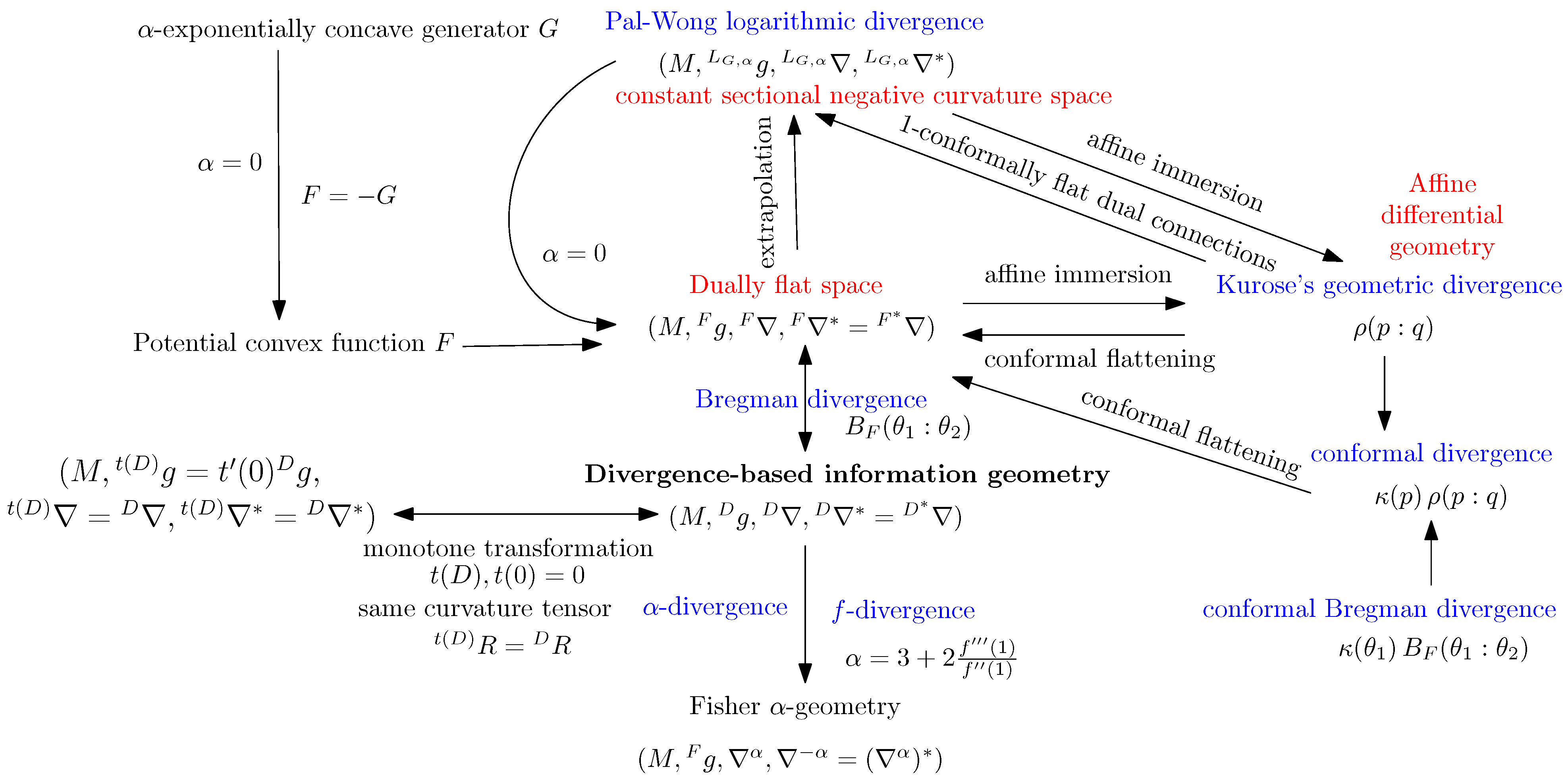
2.4. Generalized KL Divergences as Conformal Bregman Divergences on Monotone Embeddings

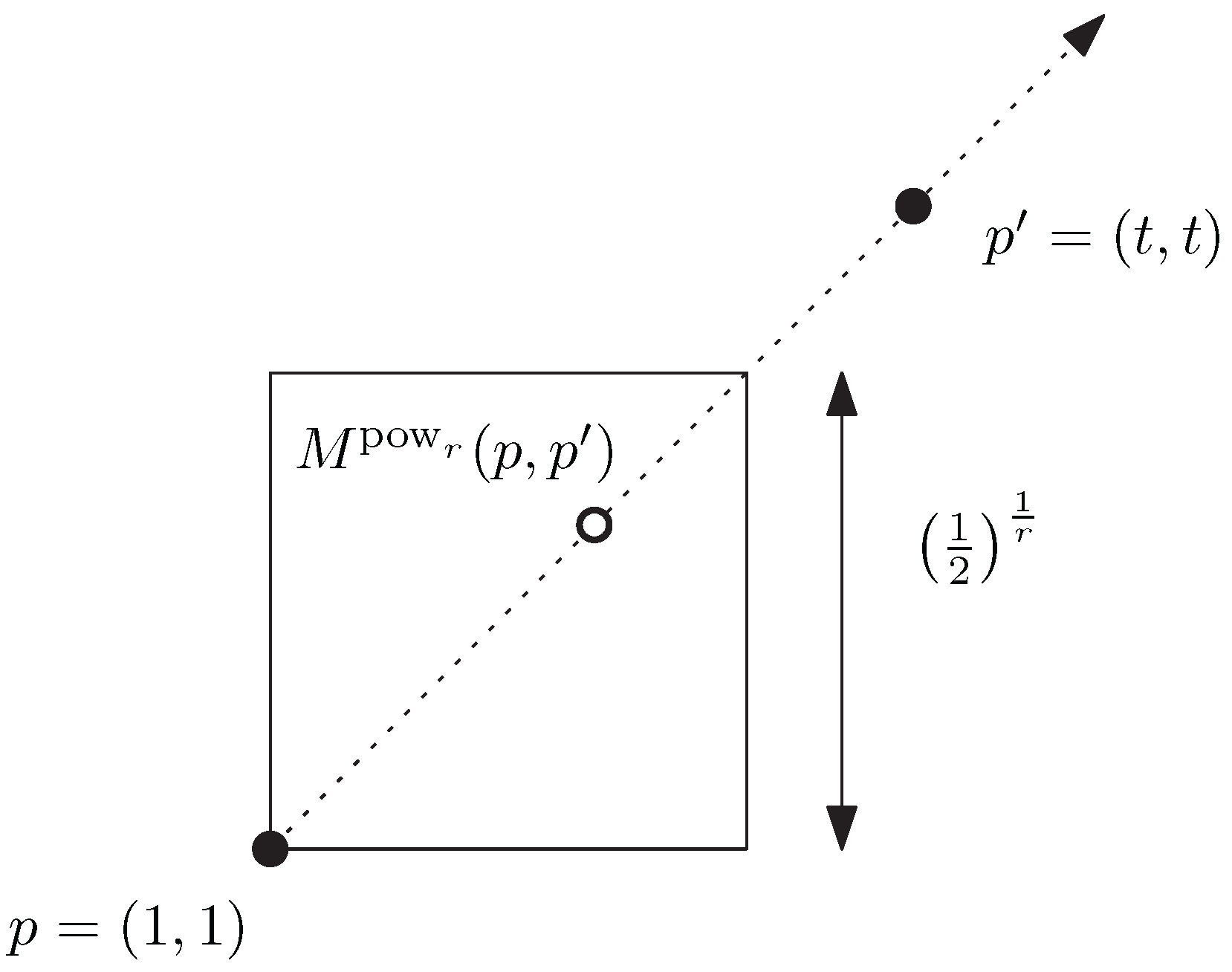
Let us rewrite the generalized KLDs $I_1^{f,g}$ as a conformal Bregman representational divergence [58,59,60] as follows:

Theorem 4.

The generalized KLDs $I_1^{f,g}$ divergences are conformal Bregman representational divergences

$$I_1^{f,g}(p:q)=\int \frac{1}{f^{\prime }\left(p\right)}{B}_F(g\left(q\right):g\left(p\right))\mathrm{d}\mu ,$$

(77)

with $F=f\circ g^{-1}$ a strictly convex and differentiable Bregman convex generator defining the scalar Bregman divergence [61] $B_F$:

$$B_F(a:b)=F\left(a\right)-F\left(b\right)-(a-b)F^{\prime }\left(b\right).$$

Proof. 

For the Bregman strictly convex and differentiable generator $F=f\circ g^{-1}$, we expand the following conformal divergence

$$\begin{array}{ccc}\hfill \frac{1}{f^{\prime }\left(p\right)}{B}_F(g\left(q\right):g\left(p\right))& =& \frac{1}{f^{\prime }\left(p\right)}\left(F\left(g\left(q\right)\right)-F\left(g\left(p\right)\right)-(g\left(q\right)-g\left(p\right))F^{\prime }\left(g\left(p\right)\right)\right),\hfill \end{array}$$

(78)

$$\begin{array}{ccc}& =& \frac{1}{f^{\prime }\left(p\right)}\left((f\left(q\right)-f\left(p\right))-(g\left(q\right)-g\left(p\right))\frac{f^{\prime }\left(p\right)}{g^{\prime }\left(p\right)}\right),\hfill \end{array}$$

(79)

since $(g^{-1}\circ g)\left(x\right)=x$ and $F^{\prime }\left(g\left(x\right)\right)=\frac{f^{\prime }\left(x\right)}{g^{\prime }\left(x\right)}$. It follows that

$$\begin{array}{ccc}\hfill \frac{1}{f^{\prime }\left(p\right)}{B}_F(g\left(q\right):g\left(p\right))& =& \frac{f\left(q\right)-f\left(p\right)}{f^{\prime }\left(p\right)}-\frac{g\left(q\right)-g\left(p\right)}{g^{\prime }\left(p\right)},\hfill \end{array}$$

(80)

$$\begin{array}{ccc}& =& E_f(p,q)-E_g(p,q)=I_1^{f,g}(p:q).\hfill \end{array}$$

(81)

Hence, we easily check that $I_1^{f,g}(p:q)=\int \frac{1}{f^{\prime }\left(p\right)}{B}_F(g\left(q\right):g\left(p\right))\mathrm{d}\mu \ge 0$ since $f^{\prime }\left(p\right)>0$ and $B_F\ge 0$. □

In general, for a functional generator f and a strictly monotonic representational function r (also called monotone embedding [62] in information geometry), we can define the representational Bregman divergence [63] $B_{f\circ r^{-1}}(r\left(p\right):r\left(q\right))$ provided that $F=f\circ r^{-1}$ is a Bregman generator (i.e., strictly convex and differentiable).

The Itakura–Saito divergence [64] (IS) between two densities p and q is defined by:

$$\begin{array}{ccc}\hfill D_{\mathrm{IS}}(p:q)& =& \int \left(\frac{p}{q}-log\frac{p}{q}-1\right)\mathrm{d}\mu ,\hfill \end{array}$$

(82)

$$\begin{array}{ccc}& =& \int D_{\mathrm{IS}}(p\left(x\right):q\left(x\right))\mathrm{d}\mu \left(x\right),\hfill \end{array}$$

(83)

where $D_{\mathrm{IS}}(x:y)=\frac{x}{y}-log\frac{x}{y}-1$ is the scalar IS divergence. This divergence was originally designed in sound processing for measuring the discrepancy between two speech power spectra. Observe that the IS divergence is invariant by rescaling: $D_{\mathrm{IS}}(tp:tq)=D_{\mathrm{IS}}(p:q)$ for any $t>0$. The IS divergence is a Bregman divergence [61] obtained for the Burg information generator (i.e., negative Burg entropy): $F_{\mathrm{Burg}}\left(u\right)=-logu$ with $F_{\mathrm{Burg}}^{\prime }\left(u\right)=-\frac{1}{u}$. It follows that we have

$$I_1^f(p:q)=\int p{B}_f(q:p)\mathrm{d}\mu ,$$

(84)

The Itakura–Saito divergence may further be extended to a family of $\alpha$-Itakura–Saito divergences (see [6], Equation (10).45 of Theorem 10.1):

$$\begin{array}{ccc}\hfill D_{\mathrm{IS},\alpha }(p:q)& =& \left\{\begin{array}{cc}\int \frac{1}{{\alpha }^2}\left({\left(\frac{p}{q}\right)}^{\alpha }-\alpha log\frac{p}{q}-1\right)\mathrm{d}\mu \hfill & \alpha \ne 0\hfill \\ \frac{1}{2}\int {(logq-logp)}^2\mathrm{d}\mu \hfill & \alpha =0.\hfill \end{array}\right.\hfill \end{array}$$

(85)

In [56], a generalization of the Bregman divergences was obtained using the comparative convexity induced by two abstract means M and N to define $(M,N)$-Bregman divergences as limit of scaled $(M,N)$-Jensen divergences. The skew $(M,N)$-Jensen divergences are defined for $\alpha \in (0,1)$ by:

$$J_{F,\alpha }^{M,N}(p:q)=\frac{1}{\alpha (1-\alpha )}\left(N_{\alpha }(F\left(p\right),F\left(q\right)))-F\left(M_{\alpha }(p,q)\right)\right),$$

(86)

where $M_{\alpha }$ and $N_{\alpha }$ are weighted means that should be regular [56] (i.e., homogeneous, symmetric, continuous, and increasing in each variable). Then, we can define the $(M,N)$-Bregman divergence as

$$\begin{array}{ccc}\hfill B_F^{M,N}(p:q)& =& \underset{\alpha \to 1^{-}}{lim}{J}_{F,\alpha }^{M,N}(p:q),\hfill \end{array}$$

(87)

$$\begin{array}{ccc}& =& \underset{\alpha \to 1^{-}}{lim}\frac{1}{\alpha (1-\alpha )}\left(N_{\alpha }(F\left(p\right),F\left(q\right)))-F\left(M_{\alpha }(p,q)\right)\right).\hfill \end{array}$$

(88)

The formula obtained in [56] for the quasi-arithmetic means $M^f$ and $M^g$ and a functional generator F that is $(M^f,M^g)$-convex is:

$$\begin{array}{ccc}\hfill B_F^{f,g}(p:q)& =& \frac{g\left(F\right(p\left)\right)-g\left(F\right(q\left)\right)}{g^{\prime }\left(F\left(q\right)\right)}-\frac{f\left(p\right)-f\left(q\right)}{f^{\prime }\left(q\right)}{F}^{\prime }\left(q\right),\hfill \end{array}$$

(89)

$$\begin{array}{ccc}& =& \frac{1}{f^{\prime }\left(F\left(q\right)\right)}{B}_{g\circ F\circ f^{-1}}(f\left(p\right):f\left(q\right))\ge 0.\hfill \end{array}$$

(90)

This is a conformal divergence [58] that can be written using the $E_f$ terms as:

$$B_F^{f,g}(p:q)=E_g(F\left(q\right),F\left(p\right))-E_f(q,p)F^{\prime }\left(q\right).$$

(91)

A function F is $(M^f,M^g)$-convex iff $g\circ F\circ f^{-1}$ is (ordinary) convex [56].

The information geometry induced by a Bregman divergence (or equivalently by its convex generator) is a dually flat space [6]. The dualistic structure induced by a conformal Bregman representational divergence is related to conformal flattening [59,60]. The notion of conformal structures was first introduced in information geometry by Okamoto et al. [65].

Following the work of Ohara [59,60,66], the Kurose geometric divergence $\rho (p,r)$ [67] (a contrast function in affine differential geometry) induced by a pair $(L,M)$ of strictly monotone smooth functions between two distributions p and r of the d-dimensional probability simplex ${\mathrm{\Delta }}_d$ is defined by (Equation (28) in [59]):

$$\rho (p:r)=\frac{1}{\mathrm{\Lambda }\left(r\right)}\sum _{i=1}^{d+1}\frac{L\left(p_i\right)-L\left(r_i\right)}{L^{\prime }\left(r_i\right)}=\frac{1}{\mathrm{\Lambda }\left(r\right)}\sum _{i=1}^{d+1}{E}_L(r_i,p_i),$$

(92)

where $\mathrm{\Lambda }\left(r\right)={\sum }_{i=1}^{d+1}\frac{1}{L^{\prime }\left(p_i\right)}{p}_i$. Affine immersions [67] can be interpreted as special embeddings.

Let $\rho$ be a divergence (contrast function) and $({}^{\rho }g,{}^{\rho }\nabla ,{}^{\rho }{\nabla }^{*})$ be the induced statistical manifold structure with

$$\begin{array}{ccc}\hfill {}^{\rho }{g}_{ij}\left(p\right)& :=& -{\left({\partial }_i\right)}_p{\left({\partial }_j\right)}_p\rho (p,q){|}_{q=p},\hfill \end{array}$$

(93)

$$\begin{array}{ccc}\hfill {\Gamma }_{ij,k}\left(p\right)& :=& -{\left({\partial }_i\right)}_p{\left({\partial }_j\right)}_p{\left({\partial }_k\right)}_q\rho (p,q){|}_{q=p},\hfill \end{array}$$

(94)

$$\begin{array}{ccc}\hfill {\Gamma }_{ij,k}^{*}\left(p\right)& :=& -{\left({\partial }_i\right)}_p{\left({\partial }_j\right)}_q{\left({\partial }_k\right)}_q\rho (p,q){|}_{q=p},\hfill \end{array}$$

(95)

where ${\left({\partial }_i\right)}_s$ denotes the tangent vector at s of a vector field ${\partial }_i$.

Consider a conformal divergence ${\rho }_{\kappa }(p:q)=\kappa \left(q\right)\rho (p:q)$ for a positive function $\kappa \left(q\right)>0$, called the conformal factor. Then, the induced statistical manifold [6,7] $({}^{{\rho }_{\kappa }}g,{}^{{\rho }_{\kappa }}\nabla ,{}^{{\rho }_{\kappa }}{\nabla }^{*})$ is 1-conformally equivalent to $({}^{\rho }g,{}^{\rho }\nabla ,{}^{\rho }{\nabla }^{*})$ and we have

$$\begin{array}{ccc}\hfill {}^{{\rho }_{\kappa }}g& =& \kappa {}^{\rho }g,\hfill \end{array}$$

(96)

$$\begin{array}{ccc}\hfill {}^{\rho }g({}^{{\rho }_{\kappa }}{\nabla }_{X}Y,Z)& =& {}^{\rho }g({}^{\rho }{\nabla }_{X}Y,Z)-d(log\kappa )\left(Z\right){}^{\rho }g(X,Y).\hfill \end{array}$$

(97)

The dual affine connections ${}^{{\rho }_{\kappa }}{\nabla }^{*}$ and ${}^{\rho }{\nabla }^{*}$ are projectively equivalent [67] (and ${}^{\rho }{\nabla }^{*}$ is said $-1$-conformally flat).

Conformal flattening [59,60] consists of choosing the conformal factor $\kappa$ such that $({}^{{\rho }_{\kappa }}g,{}^{{\rho }_{\kappa }}\nabla ,{}^{{\rho }_{\kappa }}\nabla )$ becomes a dually flat space [6] equipped with a canonical Bregman divergence.

Therefore, it follows that the statistical manifolds induced by the 1-divergence $I_1^{f,g}$ is a representational 1-conformally flat statistical manifold. Figure 1 gives an overview of the interplay of divergences with information-geometric structures. The logarithmic divergence [68] $L_{G,\alpha }$ is defined for $\alpha >0$ and an $\alpha$-exponentially concave generator G by:

$$L_{G,\alpha }({\theta }_1:{\theta }_2)=\frac{1}{\alpha }log\left(1+\alpha \nabla G{\left({\theta }_2\right)}^{\top }({\theta }_1-{\theta }_2)\right)+G\left({\theta }_2\right)-G\left({\theta }_1\right).$$

(98)

When $\alpha \to 0$, we have $L_{G,\alpha }({\theta }_1:{\theta }_2)\to B_{-G}({\theta }_1:{\theta }_2)$, where $B_F$ is the Bregman divergence [61] induced by a strictly convex and smooth function F:

$$B_F({\theta }_1:{\theta }_2)=F\left({\theta }_1\right)-F\left({\theta }_2\right)-{({\theta }_1-{\theta }_2)}^{\top }\nabla F\left({\theta }_2\right).$$

3. The Subfamily of Homogeneous $(\mathit{r},\mathit{s})$-Power $\mathbf{\alpha }$-Divergences for $\mathit{r}>\mathit{s}$

In particular, we can define the $(r,s)$-power $\alpha$-divergences from two power means $P_r=M^{{\mathrm{pow}}_r}$ and $P_s=M^{{\mathrm{pow}}_s}$ with $r>s$ (and $P_r\ge P_s$) with the family of generators ${\mathrm{pow}}_l\left(u\right)=u^l$. Indeed, we check that $f_{rs}\left(u\right):={\mathrm{pow}}_r\circ {\mathrm{pow}}_s^{-1}\left(u\right)=u^{\frac{r}{s}}$ is strictly convex on $(0,\infty )$ since $f_{rs}^{\prime \prime }\left(u\right)=\frac{r}{s}\left(\frac{r}{s}-1\right)u^{\frac{r}{s}-2}>0$ for $r>s$. Thus, $P_r$ and $P_s$ are two QAMs which are both comparable and distinct.

Table 1. Expressions of the terms $E_r$ for the family of power means $P_r$, $r\in \mathbb{R}$.

Power Mean	${\mathit{E}}_{\mathit{r}}(\mathit{p},\mathit{q})$
$P_r(r\in \mathbb{R}\backslash \left\{0\right\})$	$\frac{q^r-p^r}{r{p}^{r-1}}$
$Q(r=2)$	$\frac{q^2-p^2}{2p}$
$A(r=1)$	$q-p$
$G(r=0)$	$plog\frac{q}{p}$
$H(r=-1)$	$-p^2\left(\frac{1}{q}-\frac{1}{p}\right)=p-\frac{p^2}{q}$

lists the expressions of $E_r(p,q):=E_{{\mathrm{pow}}_r}(p,q)$ obtained from the power mean generators ${\mathrm{pow}}_r\left(u\right)=u^r$.

We conclude with the definition of the $(r,s)$-power $\alpha$-divergences:

Corollary 2

(power $\alpha$-divergences). Given $r>s$, the α-power divergences are defined for $r>s$ and $r,s\ne 0$ by

$$I_{\alpha }^{r,s}(p:q)=\left\{\begin{array}{cc}\frac{1}{\alpha (1-\alpha )}\int \left({(\alpha p^r+(1-\alpha )q^r)}^{\frac{1}{r}}-{(\alpha p^s+(1-\alpha )q^s)}^{\frac{1}{s}}\right)\mathrm{d}\mu ,\hfill & \alpha \in \mathbb{R}\backslash \{0,1\}.\hfill \\ I_1^{r,s}(p:q)=\int \left(\frac{q^r-p^r}{r{p}^{r-1}}-\frac{q^s-p^s}{s{p}^{s-1}}\right)\mathrm{d}\mu \hfill & \alpha =1,\hfill \\ I_0^{r,s}(p:q)=I_1^{r,s}(q:p)\hfill & \alpha =0.\hfill \end{array}\right.$$

(99)

When $r=0$, we get the following power $\alpha$-divergences for $s<0$:

$$I_{\alpha }^{0,s}(p:q)=\left\{\begin{array}{cc}\frac{1}{\alpha (1-\alpha )}\int \left(p^{\alpha }{q}^{1-\alpha }-{(\alpha p^s+(1-\alpha )q^s)}^{\frac{1}{s}}\right)\mathrm{d}\mu ,\hfill & \alpha \in \mathbb{R}\backslash \{0,1\}.\hfill \\ I_1^{0,s}(p:q)=\int \left(plog\frac{q}{p}-\frac{q^s-p^s}{s{p}^{s-1}}\right)\mathrm{d}\mu \hfill & \alpha =1,\hfill \\ I_0^{0,s}(p:q)=I_1^{r,s}(q:p)\hfill & \alpha =0.\hfill \end{array}\right.$$

(100)

When $s=0$, we get the following power $\alpha$-divergences for $r>0$:

$$I_{\alpha }^{r,0}(p:q)=\left\{\begin{array}{cc}\frac{1}{\alpha (1-\alpha )}\int \left({(\alpha p^r+(1-\alpha )q^r)}^{\frac{1}{r}}-p^{\alpha }{q}^{1-\alpha }\right)\mathrm{d}\mu ,\hfill & \alpha \in \mathbb{R}\backslash \{0,1\}.\hfill \\ I_1^{r,0}(p:q)=\int \left(\frac{q^r-p^r}{r{p}^{r-1}}-plog\frac{q}{p}\right)\mathrm{d}\mu \hfill & \alpha =1,\hfill \\ I_0^{r,0}(p:q)=I_1^{r,s}(q:p)\hfill & \alpha =0.\hfill \end{array}\right.$$

(101)

In particular, we get the following family of $(A,H)$$\alpha$-divergences

$$I_{\alpha }^{A,H}(p:q)=I_{\alpha }^{1,-1}(p:q)=\left\{\begin{array}{cc}\frac{1}{\alpha (1-\alpha )}\int \left(\alpha p+(1-\alpha )q-\frac{pq}{\alpha q+(1-\alpha )p}\right)\mathrm{d}\mu ,\hfill & \alpha \in \mathbb{R}\backslash \{0,1\}.\hfill \\ I_1^{1,-1}(p:q)=\int \left(q-2p+\frac{p^2}{q}\right)\mathrm{d}\mu \hfill & \alpha =1,\hfill \\ I_0^{1,-1}(p:q)=I_1^{1,-1}(q:p)\hfill & \alpha =0.\hfill \end{array}\right.,$$

(102)

and the family of $(G,H)$$\alpha$-divergences:

$$I_{\alpha }^{G,H}(p:q)=I_{\alpha }^{0,-1}(p:q)=\left\{\begin{array}{cc}\frac{1}{\alpha (1-\alpha )}\int \left(p^{\alpha }{q}^{1-\alpha }-\frac{pq}{\alpha q+(1-\alpha )p}\right)\mathrm{d}\mu ,\hfill & \alpha \in \mathbb{R}\backslash \{0,1\}.\hfill \\ I_1^{0,-1}(p:q)=\int \left(plog\frac{q}{p}-p+\frac{p^2}{q}\right)\mathrm{d}\mu \hfill & \alpha =1,\hfill \\ I_0^{0,-1}(p:q)=I_1^{0,-1}(q:p)\hfill & \alpha =0.\hfill \end{array}\right.$$

(103)

The $(r,s)$-power $\alpha$-divergences for $r,s\ne 0$ yield homogeneous divergences: $I_{\alpha }^{r,s}(tp:tq)=t{I}_{\alpha }^{r,s}(p:q)$ for any $t>0$ because the power means are homogeneous: $P_{\alpha }^r(tx,ty)=t{P}_{\alpha }^r(x,y)=tx{P}_{\alpha }^r\left(1,\frac{y}{x}\right)$. Thus, the $I_{\alpha }^{r,s}$-divergences are Csiszár f-divergences [17]

$$I_{\alpha }^{r,s}(p:q)=\int p\left(x\right)f_{r,s}\left(\frac{q\left(x\right)}{p\left(x\right)}\right)\mathrm{d}\mu$$

(104)

for the generator

$$f_{r,s}\left(u\right)=\frac{1}{\alpha (1-\alpha )}(P_{\alpha }^r(1,u)-P^s(1,u)).$$

(105)

Thus, the family of $(r,s)$-power $\alpha$-divergences are homogeneous divergences:

$$I_{\alpha }^{r,s}(tp:tq)=t{I}_{\alpha }^{r,s}(p:q),\forall t>0.$$

(106)

4. Applications to Center-Based Clustering

Clustering is a class of unsupervised learning algorithms which partitions a given d-dimensional point set $\mathcal{P}=\{p_1,\dots ,p_n\}$ into clusters such that data points falling into a same cluster tend to be more similar to data points belonging to different clusters. The celebrated k-means clustering [69] is a center-based method for clustering $\mathcal{P}$ into k clusters ${\mathcal{C}}_1,\dots ,{\mathcal{C}}_k$ (with $\mathcal{P}={\cup }_{i=1}^k{\mathcal{C}}_i$), by minimizing the following k-means objective function

$$L(\mathcal{P},\mathcal{C})=\frac{1}{n}\sum _{i=1}^n\underset{j\in \{1,\dots ,k\}}{min}{\parallel p_i-c_j\parallel }^2,$$

(107)

where the $c_j$’s denote the cluster representatives. Let $\mathcal{C}=\{c_1,\dots ,c_k\}$ denote the set of cluster centers. The cluster ${\mathcal{C}}_j$ is defined as the points of $\mathcal{P}$ closer to cluster representative $c_j$ than any other $c_i$ for $i\ne j$:

$${\mathcal{C}}_j=\{p\in \mathcal{P}:\parallel p-c_j{\parallel }^2\le \parallel p-c_l{\parallel }^2,\forall l\in \{1,\dots ,k\}\}.$$

When $k=1$, it can be shown that the centroid of the point set $\mathcal{P}$ is the unique best cluster representative:

$$arg\underset{c_1}{min}L(\mathcal{P},\left\{c_1\right\})\Rightarrow c_1=\frac{1}{n}\sum _{i=1}^n{p}_i.$$

When $d>1$ and $k>1$, finding a best partition $\mathcal{P}={\cup }_{j=1}^k{\mathcal{C}}_j$ which minimizes the objective function of Equation (107) is NP-hard [70]. When $d=1$, k-means clustering can be solved efficiently using dynamic programming [71] in subcubic $O\left(n^3\right)$ time.

The k-means objective function can be generalized to any arbitrary (potentially asymmetric) divergence $D(·:·)$ by considering the following objective function:

$$L_D(\mathcal{P},\mathcal{C}):=\frac{1}{n}\sum _{i=1}^n\underset{j\in \{1,\dots ,k\}}{min}D(p_i:c_j).$$

(108)

Thus, when $D(p:q)={\parallel p-q\parallel }^2$, one recovers the ordinary k-means clustering [69]. When $D(p:q)=B_F(p:q)$ is chosen as a Bregman divergence, one gets the right-sided Bregman k-means clustering [72] as the minimization of the cluster centers are defined on the right-sided arguments of D in Equation (108). When $F\left(x\right)={\parallel x\parallel }_2^2$, Bregman k-means clustering (i.e., $D(p:q)=B_F(p:q)$ in Equation (108)) amounts to the ordinary k-means clustering. The right-sided Bregman centroid for $k=1$ coincides with the center of mass and is independent of the Bregman generator F:

$$arg\underset{c_1}{min}{L}_{B_F}(\mathcal{P},\left\{c_1\right\})\Rightarrow c_1=\frac{1}{n}\sum _{i=1}^n{p}_i.$$

The left-sided Bregman k-means clustering is obtained by considering the right-sided Bregman centroid for the reverse Bregman divergence ${\left(B_F\right)}^{*}(p:q)=B_F(q:p)$, and the left-sided Bregman centroid [73] can be expressed as a multivariate generalization of the quasi-arithmetic mean:

$$c_1={(\nabla F)}^{-1}\left(\frac{1}{n}\sum _{i=1}^n\nabla F\left(p_i\right)\right).$$

In order to study the robustness of k-means clustering with respect to our novel family of divergences $I_{\alpha }^{f,g}$, we first study the robustness of the left-sided Bregman centroids to outliers.

4.1. Robustness of the Left-Sided Bregman Centroids

Consider two d-dimensional points $p=(p_1,\dots ,p_d)$ and $p^{\prime }=(p_1^{\prime },\dots ,p_d^{\prime })$ of a domain $\mathrm{\Theta }\subset {\mathbb{R}}^d$. The centroid of p and $p^{\prime }$ with respect to any arbitrary divergence $D(·:·)$ is by definition the minimizer of

$$L_D\left(c\right)=\frac{1}{2}D(p:c)+\frac{1}{2}D(p^{\prime }:c),$$

provided that the minimizer ${min}_{c\in \mathrm{\Theta }}{L}_D\left(c\right)$ is unique. Assume a separable Bregman divergence induced by the generator $F\left(p\right)={\sum }_{i=1}^{d}F\left(p_i\right)$. The left-sided Bregman centroid [73] of p and $p^{\prime }$ is given by the following separable quasi-arithmetic centroid:

$$c=(c_1,\dots ,c_d),$$

with

$$c_i=M^f(p_i,p_i^{\prime })=f^{-1}\left(\frac{f\left(p_i\right)+f\left(p_i^{\prime }\right)}{2}\right),$$

where $f\left(x\right)=F^{\prime }\left(x\right)$ denotes the derivative of the Bregman generator $F\left(x\right)$.

Now, fix p (say, $p=(1,\cdots ,1)\in \mathrm{\Theta }$), and let the coordinates $p_i^{\prime }$ of $p^{\prime }$ all tend to infinity: That is, point $p^{\prime }$ plays the role of an outlier data point. We use the general framework of influence functions [74] in statistics to study the robustness of divergence-based centroids. Consider the r-power mean, a quasi-arithmetic mean induced by ${\mathrm{pow}}_r\left(x\right)=x^r$ for $r\ne 0$ and by extension ${\mathrm{pow}}_0\left(x\right)=logx$ when $r=0$ (geometric mean).

When $r<0$, we check that

$$\begin{array}{ccc}\hfill \underset{p_i^{\prime }\to +\infty }{lim}{M}^{{\mathrm{pow}}_r}(p_i,p_i^{\prime })& =& \underset{p_i^{\prime }\to +\infty }{lim}{\left(\frac{1+p_i^r}{2}\right)}^{\frac{1}{r}},\hfill \end{array}$$

(109)

$$\begin{array}{ccc}& =& {\left(\frac{1}{2}\right)}^{\frac{1}{r}}<\infty .\hfill \end{array}$$

(110)

That is, the r-power mean is robust to an outlier data point when $r<0$ (see Figure 2). Note that if instead of considering the centroid, we consider the barycenter with w denoting the weight of point p and $1-w$ denoting the weight of the outlier $p^{\prime }$ for $w\in (0,1)$, then the power r-mean falls in a square box of side $w^{\frac{1}{r}}$ when $r<0$.

On the contrary, when $r>0$ or $r=0$, we have ${lim}_{p_i^{\prime }\to +\infty }{M}^{{\mathrm{pow}}_r}(p_i,p_i^{\prime })=\infty$, and the r-power mean diverges to infinity.

Thus, when $r<0$, the quasi-arithmetic centroid of $p=(1,\cdots ,1)$ and $p^{\prime }$ is contained in a bounding box of length ${\left(\frac{1}{2}\right)}^{\frac{1}{r}}$ with left corner $(1,\dots ,1)$, and the left-sided Bregman power centroid minimizing

$$\frac{1}{2}{B}_F(c:p)+\frac{1}{2}{B}_F(c:p^{\prime })$$

is robust to outlier $p^{\prime }$.

To contrast with this result, notice that the right-sided Bregman centroid [72] is always the center of mass (arithmetic mean), and therefore not robust to outliers as a single outlier data point may potentially drag the centroid to infinity.

Example 2.

Since $M^f=M^{-f}$ for any strictly smooth increasing function f, we deduce that the quasi-arithmetic left-sided Bregman centroid induced by $F\left(x\right)=-logx$ with $f\left(x\right)=F^{\prime }\left(x\right)=-x^{-1}=-\frac{1}{x}$ for $x>0$ is the harmonic mean which is robust to outliers. The corresponding Bregman divergence is the Itakura–Saito divergence [72].

Notice that it is enough to consider without loss of generality two points p and $p^{\prime }$: Indeed, the case of the quasi-arithmetic mean of $\mathcal{P}=\{p_1,\dots ,p_n\}$ and $p^{\prime }$ can be rewritten as an equivalent weighted quasi-arithmetic mean of two points $\overline{p}=M^f(p_1,\dots ,p_n)$ with weight $w=\frac{n}{n+1}$ and $p^{\prime }$ of weight $\frac{1}{n+1}$ using the replacement property of quasi-arithmetic means:

$$M^f(p_1,\dots ,p_k,p_{k+1},\dots ,p_n)=M^f(\overline{p},\dots ,\overline{p},p_{k+1},p_n)$$

where $\overline{p}=M^f(p_1,\dots ,p_k)$.

4.2. Robustness of Generalized Kullback–Leibler Centroids

The fact that the generalized KLDs are conformal representational Bregman divergences can be used to design efficient algorithms in computational geometry [60]. For example, let us consider the centroid (or barycenter) of a finite set of weighted probability measures $P_1,\dots ,P_n\ll \mu$ (with RN derivatives $p_1,\dots ,p_n$) defined as the minimizer of

$$min\sum _{i=1}^n{w}_i{I}_1^{f,g}(p_i:c),$$

where the $w_i$’s are positive weights summing up to one (${\sum }_{i=1}^n{w}_i=1$). The divergences $I_1^{f,g}(p_i:c)$ are separable. Thus, consider without loss of generality, the scalar-generalized KLDs so that we have

$$I_1^{f,g}(p:q)=\frac{1}{f^{\prime }\left(p\right)}{B}_F(g\left(q\right):g\left(p\right)),$$

where p and q are scalars.

Since the Bregman centroid is unique and always coincide with the center of mass [72]

$$c^{*}=argmin{w}_i\sum _{i=1}^n{B}_F(p_i:c)=\sum _{i=1}^n{w}_i{p}_i,$$

for positive weights $w_i$’s summing up to one, we deduce that the right-sided generalized KLD centroid

$$arg\underset{c}{min}\frac{1}{n}\sum _{i=1}^n{I}_1^{f,g}(p_i:c)=arg\underset{c}{min}\frac{1}{n}\sum _{i=1}^n\frac{1}{f^{\prime }\left(p_i\right)}{B}_F(g\left(c\right):g\left(p_i\right))$$

amounts to a left-sided Bregman centroid with un-normalized positive weights $W_i=\frac{1}{f^{\prime }\left(p_i\right)}$ for the scalar Bregman generator $F\left(x\right)=f\left(g^{-1}\left(x\right)\right)$ with $F^{\prime }\left(x\right)=\frac{f^{\prime }\left(g^{-1}\left(x\right)\right)}{g^{\prime }\left(g^{-1}\left(x\right)\right)}$. Therefore, the right-sided generalized KLD centroid $c^{*}$ is calculated for normalized weights $w_i=\frac{W_i}{{\sum }_{j=1}^n{W}_j}$ as:

$$\begin{array}{ccc}\hfill c^{*}& =& {\left(F^{\prime }\right)}^{-1}\left(\sum _{i=1}^n{w}_i{F}^{\prime }\left(g\left(p_i\right)\right)\right),\hfill \end{array}$$

(111)

$$\begin{array}{ccc}& =& {\left(F^{\prime }\right)}^{-1}\left(\sum _{i=1}^n\frac{1}{f^{\prime }\left(p_i\right){\sum }_{j=1}^n\frac{1}{f^{\prime }\left(p_j\right)}}\frac{f^{\prime }\left(p_i\right)}{g^{\prime }\left(p_i\right)}\right),\hfill \end{array}$$

(112)

$$\begin{array}{ccc}& =& {\left(F^{\prime }\right)}^{-1}\left(\sum _{i=1}^n\frac{1}{g^{\prime }\left(p_i\right){\sum }_{j=1}^n\frac{1}{f^{\prime }\left(p_j\right)}}\right).\hfill \end{array}$$

(113)

Thus, we obtain a closed-form formula when ${\left(F^{\prime }\right)}^{-1}$ is computationally tractable. For example, consider the $(r,s)$-power KLD (with $r>s$). We have $f^{\prime }\left(x\right)=r{x}^{r-1}$, $g^{\prime }\left(x\right)=s{x}^{s-1}$, $F\left(x\right)=x^{\frac{r}{s}}$, $F^{\prime }\left(x\right)=\frac{r}{s}{x}^{\frac{r-s}{s}}$ and therefore, we get ${F^{\prime }}^{-1}\left(x\right)={\left(\frac{s}{r}x\right)}^{\frac{s}{r-s}}$. Thus, we get a closed-form formula for the right-sided $(r,s)$-power Kullback–Leibler centroid using Equation (113).

Overall, we can design a k-means-type algorithm with respect to our generalized KLDs following [72]. Moreover, we can initialize probabilistically k-means with a fast k-means++ seeding [34] described in Algorithm 1. The performance of the k-means++ seeding (i.e., the ratio $\frac{L_D(\mathcal{P},\mathcal{C})}{{min}_{\mathcal{C}}{L}_D(\mathcal{P},\mathcal{C})}$) is $O(logk)$ when $D(p:q)={\parallel p-q\parallel }^2$, and the analysis has been extended to arbitrary divergences in [75]. The merit of using the k-means++ seeding is that we do not need to iteratively update the cluster representatives using Lloyd’s heuristic [69] and we can thus bypass the calculations of centroids and merely choose the cluster representatives from the source data points $\mathcal{P}$ as described in Algorithm 1.

Algorithm 1: Generic seeding of k-means with divergence-based k-means++.

input: A finite set $\mathcal{P}=\{p_1,\dots ,p_n\}$ of n points, the number of cluster    representatives $k\ge 1$, and an arbitrary divergence $D(·:·)$ Output: Set of initial cluster centers $\mathcal{C}=\{c_1,\dots ,c_k\}$ Choose $c_1\leftarrow p_i$ with uniform probability and $\mathcal{C}=\left\{c_1\right\}$ return $\mathcal{C}$

The advantage of using a conformal Bregman divergence such as a total Bregman divergence [33] or $I_1^{f,g}$ is to potentially ensure robustness to outliers (e.g., see Theorem III.2 of [33]). Robustness property of these novel $I_1^{f,g}$ divergences can also be studied for statistical inference tasks based on minimum divergence methods [4,76].

5. Conclusions and Discussion

For two comparable strict means [35] $M(p,q)\ge N(p,q)$ (with equality holding if and only if $p=q$), one can define their $(M,N)$-divergence as

$$I^{M,N}(p:q):=4\int \left(M(p,q)-N(p,q)\right)\mathrm{d}\mu .$$

(114)

When the property of strict comparable means extend to their induced weighted means $M_{\alpha }(p,q)$ and $N_{\alpha }(p,q)$ (i.e., $M_{\alpha }(p,q)\ge N_{\alpha }(p,q)$), one can further define the family of $(M,N)$$\alpha$-divergences for $\alpha \in (0,1)$:

$$I_{\alpha }^{M,N}(p:q):=\frac{1}{\alpha (1-\alpha )}\int \left(M_{1-\alpha }(p,q)-N_{1-\alpha }(p,q)\right)\mathrm{d}\mu ,$$

(115)

so that $I^{M,N}(p:q)=I_{\frac{1}{2}}^{M,N}(p:q)$. When the weighted means are symmetric, the reference duality holds (i.e., $I_{\alpha }^{M,N}(q:p)=I_{1-\alpha }^{M,N}(p:q)$), and we can define the $(M,N)$-equivalent of the Kullback–Leibler divergence, i.e., the $(M,N)$ 1-divergence, as the limit case (when it exists): $I_1^{M,N}(p:q)={lim}_{\alpha \to 1}{I}_{\alpha }^{M,N}(p:q)$. Similarly, the $(M,N)$-equivalent of the reverse Kullback–Leibler divergence is obtained as $I_0^{M,N}(p:q)={lim}_{\alpha \to 0}{I}_{\alpha }^{M,N}(p:q)$.

We proved that the quasi-arithmetic weighted means [30] $M_{\alpha }^f$ and $M_{\alpha }^g$ were strictly comparable whenever $f\circ g^{-1}$ was strictly convex. In the limit cases of $\alpha \to 0$ and $\alpha \to 1$, we reported a closed-form formula for the equivalent of the forward and the reverse Kullback–Leibler divergences. We reported closed-form formulas for the quasi-arithmetic $\alpha$-divergences $I_{\alpha }^{f,g}(p:q):=I_{\alpha }^{M^f,M^g}(p:q)$ for $\alpha \in [0,1]$ (Theorem 3) and for the subfamily of homogeneous $(r,s)$-power $\alpha$-divergences $I_{\alpha }^{r,s}(p:q):=I_{\alpha }^{M^{{\mathrm{pow}}_r},M^{{\mathrm{pow}}_s}}(p:q)$ induced by power means (Corollary 2). The ordinary $(A,G)$ $\alpha$-divergences [12], the $(A,H)$$\alpha$-divergences, and the $(G,H)$ $\alpha$-divergences are examples of $(r,s)$-power $\alpha$-divergences obtained for $(r,s)=(1,0)$, $(r,s)=(1,-1)$ and $(r,s)=(0,-1)$, respectively.

Generalized $\alpha$-divergences may prove useful in reporting a closed-form formula between densities of a parametric family $\left\{p_{\theta }\right\}$. For example, consider the ordinary $\alpha$-divergences between two scale Cauchy densities $p_1\left(x\right)=\frac{1}{\pi }\frac{s_1}{x^2+s_1^2}$ and $p_2\left(x\right)=\frac{1}{\pi }\frac{s_2}{x^2+s_2^2}$; there is no obvious closed-form for the ordinary $\alpha$-divergences, but we can report a closed-form for the $(A,H)$ $\alpha$-divergences following the calculus reported in [41]:

$$\begin{array}{ccc}\hfill I_{\alpha }^{A,H}(p_1:p_2)& =& \frac{1}{\alpha (1-\alpha )}\left(1-\int H_{1-\alpha }(p_1\left(x\right),p_2\left(x\right))\mathrm{d}\mu \left(x\right)\right),\hfill \end{array}$$

(116)

$$\begin{array}{ccc}& =& \frac{1}{\alpha (1-\alpha )}\left(1-\frac{s_1{s}_2}{(\alpha s_1+(1-\alpha )s_2)s_{1-\alpha }}\right),\hfill \end{array}$$

(117)

with $s_{\alpha }=\sqrt{\frac{\alpha s_1{s}_2^2+(1-\alpha )s_2{s}_1^2}{\alpha s_1+(1-\alpha )s_2}}$. For probability distributions $p_{{\theta }_1}$ and $p_{{\theta }_2}$ belonging to the same exponential family [77] with cumulant function F, the ordinary $\alpha$-divergences admit the following closed-form solution:

$$\begin{array}{ccc}& & I_{\alpha }(p_{{\theta }_1}:p_{{\theta }_2})=\hfill \\ & & \left\{\begin{array}{cc}\frac{1}{\alpha (1-\alpha )}\left(1-exp\left(F(\alpha {\theta }_1+(1-\alpha ){\theta }_2)-(\alpha F\left({\theta }_1\right)+(1-\alpha )F\left({\theta }_2\right)\right)\right),\hfill & \alpha \in (0,1)\hfill \\ I_1(p_{{\theta }_1}:p_{{\theta }_2})=\mathrm{KL}(p_{{\theta }_1}:p_{{\theta }_2})=B_F({\theta }_2:{\theta }_1),\hfill & \alpha =1\hfill \\ I_0(p_{{\theta }_1}:p_{{\theta }_2})=\mathrm{KL}(p_{{\theta }_2}:p_{{\theta }_1})=B_F({\theta }_1:{\theta }_2)\hfill & \alpha =0\hfill \end{array}\right.\hfill \end{array}$$

(118)

where $B_F$ is the Bregman divergence: $B_F({\theta }_2:{\theta }_1)=F\left({\theta }_2\right)-F\left({\theta }_1\right)-{({\theta }_2-{\theta }_1)}^{\top }\nabla F\left({\theta }_1\right)$.

Instead of considering ordinary $\alpha$-divergences in applications, one may consider the $(r,s)$-power $\alpha$-divergences, and tune the three scalar parameters $(r,s,\alpha )$ according to the various tasks (say, by cross-validation in supervised machine learning tasks, see [13]). For the limit cases of $\alpha \to 0$ or of $\alpha \to 1$, we further proved that the limit KL type divergences amounted to conformal Bregman divergences on strictly monotone embeddings and explained the connection of conformal divergences with conformal flattening [60], which allows one to build fast algorithms for centroid-based k-means clustering [72], Voronoi diagrams, and proximity data-structures [60,63]. Some ideas left for future directions is to study the properties of these new $(M,N)$$\alpha$-divergences for statistical inference [2,4,76].

References

1. Keener, R.W. Theoretical Statistics: Topics for a Core Course; Springer: Berlin/Heidelberg, Germany, 2011. [Google Scholar]
2. Basu, A.; Shioya, H.; Park, C. Statistical Inference: The Minimum Distance Approach; CRC Press: Boca Raton, FL, USA, 2011. [Google Scholar]
3. Basseville, M. Divergence measures for statistical data processing — An annotated bibliography. Signal Process. 2013, 93, 621–633. [Google Scholar] [CrossRef]
4. Pardo, L. Statistical Inference Based on Divergence Measures; CRC Press: Boca Raton, FL, USA, 2018. [Google Scholar]
5. Oller, J.M. Some geometrical aspects of data analysis and statistics. In Statistical Data Analysis and Inference; Elsevier: Amsterdam, The Netherlands, 1989; pp. 41–58. [Google Scholar]
6. Amari, S. Information Geometry and Its Applications; Applied Mathematical Sciences; Springer: Tokyo, Japan, 2016. [Google Scholar]
7. Eguchi, S. Geometry of minimum contrast. Hiroshima Math. J. 1992, 22, 631–647. [Google Scholar] [CrossRef]
8. Cover, T.M.; Thomas, J.A. Elements of Information Theory; John Wiley & Sons: Hoboken, NJ, USA, 2012. [Google Scholar]
9. Cichocki, A.; Amari, S.i. Families of alpha-beta-and gamma-divergences: Flexible and robust measures of similarities. Entropy 2010, 12, 1532–1568. [Google Scholar] [CrossRef] [Green Version]
10. Amari, S.i. α-Divergence is Unique, belonging to Both f-divergence and Bregman Divergence Classes. IEEE Trans. Inf. Theory 2009, 55, 4925–4931. [Google Scholar] [CrossRef]
11. Zhang, J. Divergence function, duality, and convex analysis. Neural Comput. 2004, 16, 159–195. [Google Scholar] [CrossRef]
12. Hero, A.O.; Ma, B.; Michel, O.; Gorman, J. Alpha-Divergence for Classification, Indexing and Retrieval; Technical Report CSPL-328; Communication and Signal Processing Laboratory, University of Michigan: Ann Arbor, MI, USA, 2001. [Google Scholar]
13. Dikmen, O.; Yang, Z.; Oja, E. Learning the information divergence. IEEE Trans. Pattern Anal. Mach. Intell. 2014, 37, 1442–1454. [Google Scholar] [CrossRef] [Green Version]
14. Liu, W.; Yuan, K.; Ye, D. On α-divergence based nonnegative matrix factorization for clustering cancer gene expression data. Artif. Intell. Med. 2008, 44, 1–5. [Google Scholar] [CrossRef]
15. Hellinger, E. Neue Begründung der Theorie Quadratischer Formen von Unendlichvielen Veränderlichen. J. Für Die Reine Und Angew. Math. 1909, 1909, 210–271. [Google Scholar] [CrossRef]
16. Ali, S.M.; Silvey, S.D. A general class of coefficients of divergence of one distribution from another. J. R. Stat. Soc. Ser. B 1966, 28, 131–142. [Google Scholar] [CrossRef]
17. Csiszár, I. Information-type measures of difference of probability distributions and indirect observation. Stud. Sci. Math. Hung. 1967, 2, 229–318. [Google Scholar]
18. Qiao, Y.; Minematsu, N. A study on invariance of f-divergence and its application to speech recognition. IEEE Trans. Signal Process. 2010, 58, 3884–3890. [Google Scholar] [CrossRef]
19. Li, W. Transport information Bregman divergences. Inf. Geom. 2021, 4, 435–470. [Google Scholar] [CrossRef]
20. Li, W. Transport information Hessian distances. In Proceedings of the International Conference on Geometric Science of Information (GSI), Paris, France, 21–23 July 2021; Springer: Berlin/Heidelberg, Germany, 2021; pp. 808–817. [Google Scholar]
21. Li, W. Transport information geometry: Riemannian calculus on probability simplex. Inf. Geom. 2022, 5, 161–207. [Google Scholar] [CrossRef]
22. Amari, S.i. Integration of stochastic models by minimizing α-divergence. Neural Comput. 2007, 19, 2780–2796. [Google Scholar] [CrossRef] [PubMed]
23. Cichocki, A.; Lee, H.; Kim, Y.D.; Choi, S. Non-negative matrix factorization with α-divergence. Pattern Recognit. Lett. 2008, 29, 1433–1440. [Google Scholar] [CrossRef]
24. Wada, J.; Kamahara, Y. Studying malapportionment using α-divergence. Math. Soc. Sci. 2018, 93, 77–89. [Google Scholar] [CrossRef]
25. Maruyama, Y.; Matsuda, T.; Ohnishi, T. Harmonic Bayesian prediction under α-divergence. IEEE Trans. Inf. Theory 2019, 65, 5352–5366. [Google Scholar] [CrossRef]
26. Iqbal, A.; Seghouane, A.K. An α-Divergence-Based Approach for Robust Dictionary Learning. IEEE Trans. Image Process. 2019, 28, 5729–5739. [Google Scholar] [CrossRef]
27. Ahrari, V.; Habibirad, A.; Baratpour, S. Exponentiality test based on alpha-divergence and gamma-divergence. Commun. Stat.-Simul. Comput. 2019, 48, 1138–1152. [Google Scholar] [CrossRef]
28. Sarmiento, A.; Fondón, I.; Durán-Díaz, I.; Cruces, S. Centroid-based clustering with αβ-divergences. Entropy 2019, 21, 196. [Google Scholar] [CrossRef] [Green Version]
29. Niculescu, C.P.; Persson, L.E. Convex Functions and Their Applications: A Contemporary Approach, 1st ed.; Springer Science & Business Media: Berlin/Heidelberg, Germany, 2006. [Google Scholar]
30. Kolmogorov, A.N. Sur la notion de moyenne. Acad. Naz. Lincei Mem. Cl. Sci. His. Mat. Natur. Sez. 1930, 12, 388–391. [Google Scholar]
31. Gibbs, A.L.; Su, F.E. On choosing and bounding probability metrics. Int. Stat. Rev. 2002, 70, 419–435. [Google Scholar] [CrossRef]
32. Rachev, S.T.; Klebanov, L.B.; Stoyanov, S.V.; Fabozzi, F. The Methods of Distances in the Theory of Probability and Statistics; Springer: Berlin/Heidelberg, Germany, 2013; Volume 10. [Google Scholar]
33. Vemuri, B.C.; Liu, M.; Amari, S.I.; Nielsen, F. Total Bregman divergence and its applications to DTI analysis. IEEE Trans. Med Imaging 2010, 30, 475–483. [Google Scholar] [CrossRef] [Green Version]
34. Arthur, D.; Vassilvitskii, S. k-means++: The advantages of careful seeding. In Proceedings of the SODA ’07: Proceedings of the Eighteenth Annual ACM-SIAM Symposium on Discrete Algorithms, New Orleans, LA, USA, 7–9 January 2007; Society for Industrial and Applied Mathematics: Philadelphia, PA, USA, 2007; pp. 1027–1035. [Google Scholar]
35. Bullen, P.S.; Mitrinovic, D.S.; Vasic, M. Means and Their Inequalities; Springer Science & Business Media: Berlin/Heidelberg, Germany, 2013; Volume 31. [Google Scholar]
36. Toader, G.; Costin, I. Means in Mathematical Analysis: Bivariate Means; Academic Press: Cambridge, MA, USA, 2017. [Google Scholar]
37. Cauchy, A.L.B. Cours d’analyse de l’École Royale Polytechnique; Debure frères: Paris, France, 1821. [Google Scholar]
38. Chisini, O. Sul concetto di media. Period. Di Mat. 1929, 4, 106–116. [Google Scholar]
39. Bhattacharyya, A. On a measure of divergence between two statistical populations defined by their probability distributions. Bull. Calcutta Math. Soc. 1943, 35, 99–109. [Google Scholar]
40. Nielsen, F.; Boltz, S. The Burbea-Rao and Bhattacharyya centroids. IEEE Trans. Inf. Theory 2011, 57, 5455–5466. [Google Scholar] [CrossRef] [Green Version]
41. Nielsen, F. Generalized Bhattacharyya and Chernoff upper bounds on Bayes error using quasi-arithmetic means. Pattern Recognit. Lett. 2014, 42, 25–34. [Google Scholar] [CrossRef] [Green Version]
42. Nagumo, M. Über eine klasse der mittelwerte. Jpn. J. Math. Trans. Abstr. 1930, 7, 71–79. [Google Scholar] [CrossRef] [Green Version]
43. De Finetti, B. Sul concetto di media. Ist. Ital. Degli Attuari 1931, 3, 369–396. [Google Scholar]
44. Hardy, G.; Littlewood, J.; Pólya, G. Inequalities; Cambridge Mathematical Library, Cambridge University Press: Cambridge, UK, 1988. [Google Scholar]
45. Rényi, A. On measures of entropy and information. In Proceedings of the Fourth Berkeley Symposium on Mathematical Statistics and Probability, Berkeley, CA, USA, 20 June–30 July 1960; The Regents of the University of California: Oakland, CA, USA, 1961; Volume 1. Contributions to the Theory of Statistics. [Google Scholar]
46. Holder, O.L. Über einen Mittelwertssatz. Nachr. Akad. Wiss. Gottingen Math.-Phys. Kl. 1889, 44, 38–47. [Google Scholar]
47. Bhatia, R. The Riemannian mean of positive matrices. In Matrix Information Geometry; Springer: Berlin/Heidelberg, Germany, 2013; pp. 35–51. [Google Scholar]
48. Akaoka, Y.; Okamura, K.; Otobe, Y. Bahadur efficiency of the maximum likelihood estimator and one-step estimator for quasi-arithmetic means of the Cauchy distribution. Ann. Inst. Stat. Math. 2022, 74, 1–29. [Google Scholar] [CrossRef]
49. Kim, S. The quasi-arithmetic means and Cartan barycenters of compactly supported measures. Forum Math. Gruyter 2018, 30, 753–765. [Google Scholar] [CrossRef]
50. Carlson, B.C. The logarithmic mean. Am. Math. Mon. 1972, 79, 615–618. [Google Scholar] [CrossRef]
51. Stolarsky, K.B. Generalizations of the logarithmic mean. Math. Mag. 1975, 48, 87–92. [Google Scholar] [CrossRef]
52. Jarczyk, J. When Lagrangean and quasi-arithmetic means coincide. J. Inequal. Pure Appl. Math. 2007, 8, 71. [Google Scholar]
53. Páles, Z.; Zakaria, A. On the Equality of Bajraktarević Means to Quasi-Arithmetic Means. Results Math. 2020, 75, 19. [Google Scholar] [CrossRef] [Green Version]
54. Maksa, G.; Páles, Z. Remarks on the comparison of weighted quasi-arithmetic means. Colloq. Math. 2010, 120, 77–84. [Google Scholar] [CrossRef]
55. Zhang, J. Nonparametric information geometry: From divergence function to referential-representational biduality on statistical manifolds. Entropy 2013, 15, 5384–5418. [Google Scholar] [CrossRef] [Green Version]
56. Nielsen, F.; Nock, R. Generalizing Skew Jensen Divergences and Bregman Divergences with Comparative Convexity. IEEE Signal Process. Lett. 2017, 24, 1123–1127. [Google Scholar] [CrossRef]
57. Kuczma, M. An Introduction to the Theory of Functional Equations and Inequalities: Cauchy’s Equation and Jensen’s Inequality; Springer Science & Business Media: Berlin/Heidelberg, Germany, 2009. [Google Scholar]
58. Nock, R.; Nielsen, F.; Amari, S.i. On conformal divergences and their population minimizers. IEEE Trans. Inf. Theory 2015, 62, 527–538. [Google Scholar] [CrossRef] [Green Version]
59. Ohara, A. Conformal flattening for deformed information geometries on the probability simplex. Entropy 2018, 20, 186. [Google Scholar] [CrossRef] [Green Version]
60. Ohara, A. Conformal Flattening on the Probability Simplex and Its Applications to Voronoi Partitions and Centroids. In Geometric Structures of Information; Springer: Berlin/Heidelberg, Germany, 2019; pp. 51–68. [Google Scholar]
61. Bregman, L.M. The relaxation method of finding the common point of convex sets and its application to the solution of problems in convex programming. USSR Comput. Math. Math. Phys. 1967, 7, 200–217. [Google Scholar] [CrossRef]
62. Zhang, J. On monotone embedding in information geometry. Entropy 2015, 17, 4485–4499. [Google Scholar] [CrossRef] [Green Version]
63. Nielsen, F.; Nock, R. The dual Voronoi diagrams with respect to representational Bregman divergences. In Proceedings of the Sixth International Symposium on Voronoi Diagrams (ISVD), Copenhagen, Denmark, 23–26 June 2009; IEEE: Piscataway, NJ, USA, 2009; pp. 71–78. [Google Scholar]
64. Itakura, F.; Saito, S. Analysis synthesis telephony based on the maximum likelihood method. In Proceedings of the 6th International Congress on Acoustics, Tokyo, Japan, 21–28 August 1968; pp. 280–292. [Google Scholar]
65. Okamoto, I.; Amari, S.I.; Takeuchi, K. Asymptotic theory of sequential estimation: Differential geometrical approach. Ann. Stat. 1991, 19, 961–981. [Google Scholar] [CrossRef]
66. Ohara, A.; Matsuzoe, H.; Amari, S.I. Conformal geometry of escort probability and its applications. Mod. Phys. Lett. B 2012, 26, 1250063. [Google Scholar] [CrossRef]
67. Kurose, T. On the divergences of 1-conformally flat statistical manifolds. Tohoku Math. J. Second Ser. 1994, 46, 427–433. [Google Scholar] [CrossRef]
68. Pal, S.; Wong, T.K.L. The geometry of relative arbitrage. Math. Financ. Econ. 2016, 10, 263–293. [Google Scholar] [CrossRef]
69. Lloyd, S. Least squares quantization in PCM. IEEE Trans. Inf. Theory 1982, 28, 129–137. [Google Scholar] [CrossRef] [Green Version]
70. Mahajan, M.; Nimbhorkar, P.; Varadarajan, K. The planar k-means problem is NP-hard. Theor. Comput. Sci. 2012, 442, 13–21. [Google Scholar] [CrossRef] [Green Version]
71. Wang, H.; Song, M. Ckmeans.1d.dp: Optimal k-means clustering in one dimension by dynamic programming. R J. 2011, 3, 29. [Google Scholar] [CrossRef] [Green Version]
72. Banerjee, A.; Merugu, S.; Dhillon, I.S.; Ghosh, J.; Lafferty, J. Clustering with Bregman divergences. J. Mach. Learn. Res. 2005, 6, 1705–1749. [Google Scholar]
73. Nielsen, F.; Nock, R. Sided and symmetrized Bregman centroids. IEEE Trans. Inf. Theory 2009, 55, 2882–2904. [Google Scholar] [CrossRef] [Green Version]
74. Ronchetti, E.M.; Huber, P.J. Robust Statistics; John Wiley & Sons: Hoboken, NJ, USA, 2009. [Google Scholar]
75. Nielsen, F.; Nock, R. Total Jensen divergences: Definition, properties and clustering. In Proceedings of the 2015 IEEE International Conference on Acoustics, Speech and Signal Processing (ICASSP), South Brisbane, Australia, 19–24 April 2015; IEEE: Piscataway, NJ, USA, 2015; pp. 2016–2020. [Google Scholar]
76. Eguchi, S.; Komori, O. Minimum Divergence Methods in Statistical Machine Learning; Springer: Berlin/Heidelberg, Germany, 2022. [Google Scholar]
77. Kailath, T. The divergence and Bhattacharyya distance measures in signal selection. IEEE Trans. Commun. Technol. 1967, 15, 52–60. [Google Scholar] [CrossRef]
Figure 1. Interplay of divergences and their information-geometric structures: Bregman divergences are canonical divergences of dually flat structures, and the α -logarithmic divergences are canonical divergences of 1-conformally flat statistical manifolds. When α 0 , the logarithmic divergence L F , α tends to the Bregman divergence B F .
Algorithms 15 00435 g001
Figure 2. Illustration of the robustness property of the r-power mean M pow r ( p , p ) when r < 0 for two points: a prescribed point p = ( 1 , 1 ) and an outlier point p = ( t , t ) . When t + , the r-power mean of p and p for r < 0 (e.g., coordinatewise harmonic mean when r = 1 ) is contained inside the box anchored at p of size length 1 2 1 r . The r-power mean can be interpreted as a left-sided Bregman centroid for F ( x ) = x r , i.e., F ( x ) = 1 r x r + 1 when r < 1 and F ( x ) = log x when r = 1 .
Algorithms 15 00435 g002