Unrelated Parallel Machine Scheduling with Job and Machine Acceptance and Renewable Resource Allocation

Abstract

In this paper, an unrelated parallel machine scheduling problem with job (product) and machine acceptance and renewable resource constraints was considered. The main idea of this research was to establish a production facility without (or with minimum) investment in machinery, equipment, and location. This problem can be applied to many real problems. The objective was to maximize the net profit; that is, the total revenue minus the total cost, including fixed costs of jobs, job transportation costs, renting costs of machines, renting cost of resources, and transportation costs of resources. A mixed-integer linear programming (MILP) model and several heuristics (greedy, GRASP, and simulated annealing) are presented to solve the problem.

1. Introduction

Unrelated parallel machine scheduling is the most general setting of parallel machine scheduling, where n non-preemptive jobs, all available at time zero, have to be processed on m machines. Each job can be processed by any free machine; however, the processing of job j on machine i takes an amount of time that has no relation to the processing times on the other machines. It is assumed that all of the machines are capable of processing all jobs; nevertheless, if a given machine is not capable of processing a given job, the corresponding processing time can be set to a very large value [1].

In this paper, an unrelated parallel machine scheduling problem with job (product) and machine acceptance and with renewable resources (such as manpower, industrial machines or tools, and computing devices) was considered. The main idea of this research was to establish a production facility without (or with a minimum) capital or infrastructure. The machines and resources required for processing the jobs were rented during their operating time. Each machine or resource can be rented for only one time interval, i.e., even for their idle times, the renting cost should be paid. Multiple resources of a given type can be used. The problem is to determine:

• The set of accepted jobs, considering their revenue, required processing times and resources, fixed costs, transportation costs, and penalty costs for rejected jobs;
• The set of machines that will be rented, taking into account their rent cost per time unit;
• The set of resource units that will be rented, taking into account their rent cost per time unit and transportation times and costs (typically tools or manpower);
• The time intervals for renting the selected machines;
• The time intervals for renting the selected renewable resource units;
• The assignment of the selected jobs to the selected machines;
• The start dates for processing the selected jobs.

The objective is to maximize the net profit, which is composed of revenues and costs. The revenues are given by the selected jobs, and the costs are composed of the penalties of rejected jobs and various costs of the selected jobs. The latter include the fixed costs of jobs, transportation costs (jobs and resources), and rent costs (machines and resources).

The real-case application motivating this study comes from a small company renting co-working spaces in different locations and employing freelance programmers. We are, however, unable to divulge the name of the company, nor all of the details of its operations. Broadly speaking, the company acts as a subcontractor in the software development field. From a scheduling perspective, the jobs correspond to software projects, the machines correspond to co-working sites, and the resources correspond to the programmers, grouped based on their core competences. Each time a co-working site is used, the space needs to be set up for the freelancers, hence the initial transportation time and cost. Projects are also taken in batches, motivating the use of penalties when jobs are not carried out in the allotted time frame. Furthermore, we extended certain aspects of the problem, such as including processing times depending on the selected machine, which was not the case in the original case study.

The scheduling problem with job acceptance (also called “job selection” or “job rejection”) has been studied by many papers in the literature [2,3,4,5,6,7,8]. The scheduling problem with machine acceptance (called “not-all-machines” or “optional machines”) has also been investigated by many researchers [9,10,11,12,13,14,15,16,17,18,19]. The scheduling problem with renewable resource constraints has also been widely studied in the literature due to its wide applicability to real problems [20,21,22,23,24,25,26,27]. A cross-disciplinary survey on this subject may be found in [28]. In many production and non-production organizations, the response time to the customer demand is very important and is considered as a competitive advantage. One of the very important factors affecting the response time to the customer is the transportation time. Consequently, many researchers focus on the integrated transportation and production planning/scheduling problems [29,30,31]. A survey of integrated production scheduling and outbound distribution models is presented in [32], and a review of literature on the production routing problem (PRP) can be found in [33].

To the best of our knowledge, the scheduling problem with all four mentioned features, i.e., job and machine acceptance, and renewable resource and transportation constraints, has never been studied in the past. Only the contributions in [9,13], which consider both the job and machine selection in a parallel machine environment, are very similar to our research; however, the renewable resource and job and resource transportation constraints are additionally taken into account in this paper. This problem is strongly NP-hard, since the parallel machine scheduling problem with a fixed number of machines and jobs and without resource constraints is already strongly $\mathcal{NP}$-hard [34].

The remainder of the paper is organized as follows. We begin by presenting the problem in Section 2 through the aid of an illustrative example. We then continue with an exact resolution approach based on mixed-integer linear programming and with several heuristic approaches in Section 3. In Section 4, we evaluate these approaches using artificially generated datasets (available on request), before finishing with several concluding remarks in Section 5.

2. The Problem

As mentioned previously, we consider the problem of unrelated parallel machine scheduling with job and machine acceptance as well as resource allocation and transportation constraints. This type of problem can be used in the context of establishing a production facility without capital or with little capital and no infrastructure. Both machines and resources are rented, while resources need to be transported to and between fixed machine locations. Jobs are transported to machine locations but not between machines because they can be operated in parallel.

Let us first describe several parameters that are used to define our problem. We begin with the general parameters below:

• n, the number of jobs ($j=1,\dots ,n$);
• m, the number of machines ($i=1,\dots ,m$);
• k, the number of resource types ($r=1,\dots ,k$);
• $l_r$, the number units of a resource type r ($q=1,\dots ,l_r$).

Next, we have the parameters that define a job, $\forall j\in 1\dots n$:

• $p_j$, the selling price of job j;
• $p{c}_j$, the penalty cost of not selecting job j;
• $f{c}_j$, the fixed cost of handling job j;
• $d_j$, the due date of job j; finishing the job after this date incurs a tardiness penalty;
• $t{c}_j$, the tardiness cost of job j per unit of time;
• ${\tilde{d}}_j$, the deadline of job j; a job cannot be finished after this date.

We continue with the parameters that define a machine, $\forall i\in 1\dots m$:

• $rc{m}_i$, the renting cost of machine i per unit of time;
• $mwt{m}_i$, the minimum renting time of machine i. A machine can be rented for a shorter period of time; however, a minimum renting cost proportional to $mwt{m}_i$ will need to be paid.

Next, we have the parameters that define the resource types, $\forall r\in 1\cdots k$:

• $rc{r}_r$, the renting cost of resource type r per unit of time;
• $trc{r}_r$, the cost of transporting resource r between any two machines;
• $trt{r}_r$, the time needed to transport resource r between any two machines;

Several parameters depend on both the jobs and the machines, such as, $\forall i\in 1\dots m$, $\forall j\in 1\dots n$:

• $t_{ij}$, the processing time of job j on machine i;
• $trc{j}_{ij}$, the cost of transporting job j to machine i;
• $trt{j}_{ij}$, the time for transporting job j to machine i.

Finally, a single parameter concerns both the jobs and the resources, $\forall j\in 1\dots n$, $\forall r\in 1\cdots k$:

• $a_{jr}$, a binary indicator for job j requiring resource type r in order to be processed.

In order to illustrate the problem, we consider the following example.

An event-planning company rents one or multiple venues in order to set up different events while, at the same time, taking care of contracting and transporting the performers. Following a bidding process, the company is awarded four events (jobs in a scheduling context) ($n=4$), and three venues (machines in a scheduling context) are available to be rented in its area ($m=3$). Each event requires one or multiple performers of different categories, such as opera singers and symphony bands, which can be considered as resources in a scheduling context. Therefore, up to two types of resources ($k=2$) are needed, with two opera singers and three symphony bands currently being available to our event planning company ($l_1=2$ and $l_2=3$).

Each job comes with its offer revenue and its set-up costs, but also the associated running costs. Furthermore, as these jobs have been awarded to the company, a penalty fee will be incurred if the job is forfeit. Each job comes with a due date for delivery, after which, penalties will be incurred by our company, as well as a hard deadline. These parameters may be found in

Table 1. Event (job) parameters for the illustrative example.

Jobs	J1	J2	J3	J4
Profit (p)	100 k	80 k	150 k	120 k
Penalty ($pc$)	1500	5000	2500	2000
Fixed cost ($fc$)	10 k	15 k	10 k	12.5 k
Due date (d)	15	20	12	22
Tardiness cost ($tc$)	500	700	1000	800
Deadline ($\tilde{d}$)	32	28	20	45

.

Each venue comes with a rent cost per day together with a minimum rent duration. The opera singers and symphony bands also have a daily cost, and furthermore require a certain number of days and a cost in order to be transported and set up in a new location. These elements may be found in

Table 2. Venue (machine) parameters for the illustrative example.

Venue	M1	M2	M3
Rental cost ($rcm$)	500	750	650
Minimum rental period in days ($mwtm$)	25	35	25

and

Table 3. Performer (resource) parameters for the illustrative example.

Performer	Opera Singer	Symphony Band
Rental cost ($rcr$)	1000	1500
Setup cost ($trcr$)	1500	2500
Setup time in days ($trtr$)	5	10

.

Each event has a number of performance days needed, presented in

Table 4. Performance time, in days, for each event and each venue (or processing time).

t	J1	J2	J3	J4
M1	25	30	20	35
M2	15	10	10	20
M3	35	30	20	40

.

The company also considers the time and costs needed for the initial setup of each venue for each event. Once a venue is set up, the time needed to switch to another event is considered negligible. The setup costs (or transport costs in the general case) are given in

Table 5. Initial setup (or transport) costs of locations.

trcj	J1	J2	J3	J4
M1	1000	1500	1500	2000
M2	2500	1000	1500	2000
M3	1500	3000	2000	1000

, whereas the setup times (or transport times in the general case) are given in

Table 6. Initial setup (or transport) times ($trtj$).

trtj	J1	J2	J3	J4
M1	5	10	5	5
M2	10	15	10	15
M3	5	5	10	10

.

Finally, each event may require one or both types of resources as presented in

Table 7. Event resource requirements.

a	J1	J2	J3	J4
Opera singer	1	0	1	1
Symphony band	0	1	1	1

.

Notice that J3 and J4 require both resource types, whereas the other jobs only require one.

The optimal solution for this problem is illustrated below. We begin by presenting the solution elements in

Table 8. Solution indicating start and completion dates of events and venue and resource assignments.

Jobs		J1	J2	J3	J4
Start		5	-	10	20
End		30	-	20	40
Venue		M1	-	M2	M2
Resource	Opera singer	R1,1	-	-	R1,2
	Symphony band	-	-	R2,1	R2,1

, including the start and complete times of jobs, followed by the venue and resource assignments.

We have also used several Gantt charts, starting with the one indicating the locations use in Figure 1.

Notice that only the first two venues are used. Furthermore, the second job does not appear at all, meaning that it was not selected. This may be due to it having a small profit, a relatively short deadline, and long initial setup times for the first two venues. Furthermore, as illustrated below, adding J2 would require mobilizing a second symphony band, therefore further increasing the costs.

We investigate the resource use by looking at Figure 2 and Figure 3.

We observe that only two opera singers and one symphony band are used.

The overall profit (or fitness of the solution) is $159,350$, and is given by:

• The income from selected jobs, i.e., all except the second one ($370,000$);
• The fixed costs of selected jobs ($-32,500$);
• The penalty cost of rejected jobs, i.e., the second one ($-5000$);
• The tardiness cost of late jobs, i.e., $15\times 500$ for J1, $8\times 1000$ for J3, and $18\times 800$ ($-29,900$);
• The renting cost of venues, corresponding to 25 days for the first venue and 35 days for the second, as it is used for 30 only when the minimum required is 35 ($-38,750$);
• The renting cost of resources, i.e., $(25+20)\times 1000$ for the opera singers and $(10+30)\times 1500$ for the symphony band ($-105,000$);
• The initial setup costs (or transport costs) of venues, i.e., $2\times 1500$ for the two opera singers and 2500 for the symphony band ($-5500$);
• The transfer costs of resources between venues, which amount to 0 since all resources are set up and stay in only one location (0).

3. Resolution Approaches

3.1. Exact Approach

We present, in this subsection, the mixed-integer linear program (MILP) proposed for solving the presented problem.

The variables of the model are presented in

Table 9. Variables of the MILP.

$X_j$	binary	:	1 if job j is selected and 0 otherwise, $\forall j\in 1\dots n$
$T_j$	continuous	:	tardiness of job j, $\forall j\in 1\dots n$
$W_i$	binary	:	1 if machine i is used for some jobs and 0 otherwise, $\forall i\in 1\dots m$
$Y_{ij}$	binary	:	1 if job j is processed on machine i and 0 otherwise,
			$\forall i\in 1\dots m$, $\forall j\in 1\dots n$
$C_{ij}$	continuous	:	completion time of job j on machine i, $\forall i\in 1\dots m$, $\forall j\in 1\dots n$
$ST{M}_i$	continuous	:	starting time of renting machine i, $\forall i\in 1\dots m$
$FT{M}_i$	continuous	:	finishing time of renting machine i, $\forall i\in 1\dots m$
$RT{M}_i$	continuous	:	renting time of machine i, $\forall i\in 1\dots m$
$ST{R}_{rq}$	continuous	:	starting time of renting resource q of type r, $\forall r\in 1\dots k$, $\forall q\in 1\dots l_r$
$FT{R}_{rq}$	continuous	:	finishing time of renting resource q of type r, $\forall r\in 1\dots k$, $\forall q\in 1\dots l_r$
$NT{R}_{rq}$	continuous	:	number of transfers of resource q of type r between machines,
			$\forall r\in 1\dots k$, $\forall q\in 1\dots l_r$
$Z_{irq}$	binary	:	1 if machine i uses resource q of type r to process some jobs
			and 0 otherwise, $\forall i\in 1\dots m$, $\forall r\in 1\dots k$, $\forall q\in 1\dots l_r$
$V_{j{j}^{\prime }}$	binary	:	1 if job j precedes job $j^{\prime }$ when both use the same machine
			and 0 otherwise, $\forall j,j^{\prime }\in 1\dots n,j<j^{\prime }$
$U_{i{i}^{\prime }rq}$	binary	:	1 if resource q of type r is used by machine i before machine $i^{\prime }$,
			and 0 otherwise
			$\forall i,i^{\prime }\in 1\dots m$, $i<i^{\prime }$, $\forall r\in 1\dots k$, $\forall q\in 1\dots l_r$
$G_{jrq}$	binary	:	1 if job j uses resource q of type r and 0 otherwise
			$\forall j\in 1\dots n$, $\forall r\in 1\dots k$, $\forall q\in 1\dots l_r$

.

The MILP can be formulated as follows:

$$\begin{array}{cc}\hfill max& {\displaystyle \sum _{j=1}^n{p}_j{X}_j - \sum _{j=1}^{n}f{c}_j{X}_j - \sum _{j=1}^{n}t{c}_j{T}_j - \sum _{j=1}^{n}p{c}_j\left(1X_j\right) - }\hfill \\ \hfill & {\displaystyle v\sum _{i=1}^{m}rc{m}_{i}RT{M}_i - \sum _{r=1}^k\sum _{q=1}^{l_r}rc{r}_r\left(FT{R}_{rq}ST{R}_{rq}\right) - }\hfill \\ \hfill & {\displaystyle \sum _{j=1}^n\sum _{i=1}^{m}trc{j}_{ij}{Y}_{ij} - \sum _{r=1}^k\sum _{q=1}^{l_r}trc{r}_{r}NT{R}_{rq}}\hfill \end{array}$$

(1)

s.t.:

$$\begin{array}{ccc}\hfill & Y_{ij}⩽Z_{irq}+(1 - G_{jrq})\hfill & \hfill \forall i\in 1\dots m,\forall j\in 1\dots n,\forall r\in 1\dots k,\forall q\in 1\dots l_r\end{array}$$

(2)

$$\begin{array}{ccc}\hfill & {\displaystyle NT{R}_{rq}⩾\sum _{i=1}^n{Z}_{irq} - 1}\hfill & \hspace{1em}\hspace{1em}\hspace{1em}\hspace{1em}\hspace{1em}\hspace{1em}\hspace{1em}\hspace{1em}\hspace{1em}\hspace{1em}\forall r\in 1\dots k,\forall q\in 1\dots l_r\hfill \end{array}$$

(3)

$$\begin{array}{c}{C}_{i^{\prime }{j}^{\prime }}+trt{r}_r⩽C_{ij} - t_{ij}+M\left(4Y_{ij}{Y}_{i^{\prime }{j}^{\prime }}{G}_{jrq}{G}_{j^{\prime }rq}\right)+M{U}_{i{i}^{\prime }rq}\hfill \\ \hspace{1em}\hspace{1em}\forall i,i^{\prime }\in 1\dots m,i<i^{\prime },\forall j,j^{\prime }\in 1\dots n,j<j^{\prime },\forall r\in 1\dots k,\forall q\in 1\dots l_r\hfill \end{array}$$

(4)

$$\begin{array}{c}{C}_{ij}+trt{r}_r⩽C_{i^{\prime }{j}^{\prime }}{t}_{i^{\prime }{j}^{\prime }}+M(4 - Y_{ij} - Y_{i^{\prime }{j}^{\prime }} - G_{jrq} - G_{j^{\prime }rq})+M(1 - U_{i{i}^{\prime }rq})\hfill \\ \hspace{1em}\hspace{1em}\forall i,i^{\prime }\in 1\dots m,i<i^{\prime },\forall j,j^{\prime }\in 1\dots n,j<j^{\prime },\forall r\in 1\dots k,\forall q\in 1\dots l_r\hfill \end{array}$$

(5)

$$\begin{array}{c}{\displaystyle ST{R}_{rq}⩽\sum _{i=1}^m{C}_{ij} - \sum _{i=1}^m{t}_{ij}{Y}_{ij}+M(1 - G_{jrq})}\hfill \\ \hfill & \hfill \forall j\in 1\dots n,\forall r\in 1\dots k,\forall q\in 1\dots l_r\end{array}$$

(6)

$$\begin{array}{ccc}\hfill & {\displaystyle FT{R}_{rq}⩾\sum _{i=1}^m{C}_{ij} - M(1 - G_{jrq})}\hfill & \hfill \hspace{1em}\hspace{1em}\hspace{1em}\forall j\in 1\dots n,\forall r\in 1\dots k,\forall q\in 1\dots l_r\end{array}$$

(7)

$$\begin{array}{cc}\hfill & C_{ij} - t_{ij}⩾C_{i{j}^{\prime }} - M{V}_{j{j}^{\prime }} - M(2 - Y_{ij} - Y_{i{j}^{\prime }})\hfill \\ \hfill & \hfill & \hfill \forall i\in 1\dots m,\forall j,j^{\prime }\in 1\dots n,j<j^{\prime }\end{array}$$

(8)

$$\begin{array}{cc}\hfill & C_{i{j}^{\prime }} - t_{i{j}^{\prime }}⩾C_{ij} - M(1 - V_{j{j}^{\prime }}) - M(2 - Y_{ij} - Y_{i{j}^{\prime }})\hfill \\ \hfill & \hfill & \hfill \forall i\in 1\dots m,\forall j,j^{\prime }\in 1\dots n,j<j^{\prime }\end{array}$$

(9)

$$\begin{array}{ccc}\hfill & {\displaystyle \sum _{j=1}^n{Y}_{ij}⩽n{W}_i}\hfill & \hfill \hspace{1em}\hspace{1em}\hspace{1em}\hspace{1em}\hspace{1em}\hspace{1em}\hspace{1em}\hspace{1em}\hspace{1em}\hspace{1em}\hspace{1em}\hspace{1em}\hspace{1em}\hspace{1em}\hspace{1em}\forall i\in 1\dots m\end{array}$$

(10)

$$\begin{array}{ccc}\hfill & ST{M}_i⩽C_{ij} - t_{ij}+M(1 - Y_{ij})\hfill & \hfill \hspace{1em}\hspace{1em}\hspace{1em}\forall i\in 1\dots m,\forall j\in 1\dots n\end{array}$$

(11)

$$\begin{array}{ccc}\hfill & FT{M}_i⩾C_{ij} - M(1 - Y_{ij})\hfill & \hfill \hspace{1em}\hspace{1em}\hspace{1em}\hspace{1em}\hspace{1em}\forall i\in 1\dots m,\forall j\in 1\dots n\end{array}$$

(12)

$$\begin{array}{ccc}\hfill & {\displaystyle \sum _{i=1}^m{Y}_{ij}=X_j}\hfill & \hfill \hspace{1em}\hspace{1em}\hspace{1em}\hspace{1em}\hspace{1em}\hspace{1em}\hspace{1em} \hspace{1em}\hspace{1em}\hspace{1em}\hspace{1em}\forall i\in 1\dots m,\forall j\in 1\dots n\end{array}$$

(13)

$$\begin{array}{cc}\hfill \sum _{i=1}^m{C}_{i{j}^{\prime }}⩽\sum _{i=1}^m{C}_{ij} - \sum _{i=1}^m{t}_{ij}{Y}_{ij}& +M(2 - G_{jrq} - G_{j^{\prime }rq})+M{V}_{j{j}^{\prime }}\hfill \\ & \forall j,j^{\prime }\in 1\dots n,j<j^{\prime },\forall r\in 1\dots k,\forall q\in 1\dots l_r\hfill \end{array}$$

(14)

$$\begin{array}{cc}\hfill \sum _{i=1}^m{C}_{ij}⩽\sum _{i=1}^m{C}_{i{j}^{\prime }} - \sum _{i=1}^m{t}_{i{j}^{\prime }}{Y}_{i{j}^{\prime }}& +M(2 - G_{jrq} - G_{j^{\prime }rq})+M(1 - V_{j{j}^{\prime }})\hfill \\ & \forall j,j^{\prime }\in 1\dots n,j<j^{\prime },\forall r\in 1\dots k,\forall q\in 1\dots l_r\hfill \end{array}$$

(15)

$$\begin{array}{ccc}\hfill & {\displaystyle \sum _{i=1}^m{C}_{ij}-\sum _{i=1}^m(t_{ij}+trt{j}_{ij})Y_{ij}⩾0}\hfill & \hfill \hspace{1em}\hspace{1em}\hspace{1em}\hspace{1em}\hspace{1em}\hspace{1em}\hspace{1em}\forall j\in 1\dots n\end{array}$$

(16)

$$\begin{array}{ccc}\hfill & {\displaystyle \sum _{i=1}^m{C}_{ij}⩽{\tilde{d}}_j}\hfill & \hfill \hspace{1em}\hspace{1em}\hspace{1em}\hspace{1em}\hspace{1em}\hspace{1em}\hspace{1em}\hspace{1em}\hspace{1em}\hspace{1em}\hspace{1em}\hspace{1em}\hspace{1em}\hspace{1em}\hspace{1em}\forall j\in 1\dots n\end{array}$$

(17)

$$\begin{array}{ccc}\hfill & C_{ij}⩽M{Y}_{ij}\hfill & \hfill \hspace{1em}\hspace{1em}\hspace{1em}\hspace{1em}\hspace{1em}\hspace{1em}\hspace{1em} \hspace{1em}\hspace{1em}\hspace{1em}\hspace{1em}\forall i\in 1\dots m,\forall j\in 1\dots n\end{array}$$

(18)

$$\begin{array}{ccc}\hfill & {\displaystyle T_j⩾\sum _{i=1}^m{C}_{ij} - d_j}\hfill & \hfill \hspace{1em}\hspace{1em}\hspace{1em}\hspace{1em}\hspace{1em}\hspace{1em}\hspace{1em}\hspace{1em}\hspace{1em}\hspace{1em}\hspace{1em}\hspace{1em}\hspace{1em}\forall j\in 1\dots n\end{array}$$

(19)

$$\begin{array}{ccc}\hfill & T_j⩾0\hfill & \hfill \hspace{1em}\hspace{1em}\hspace{1em}\hspace{1em}\hspace{1em}\hspace{1em}\hspace{1em}\hspace{1em}\hspace{1em}\hspace{1em}\hspace{1em}\hspace{1em}\hspace{1em}\hspace{1em}\hspace{1em}\hspace{1em}\hspace{1em}\forall j\in 1\dots n\end{array}$$

(20)

$$\begin{array}{ccc}\hfill & FT{M}_i⩾ST{M}_i\hfill & \hfill \hspace{1em}\hspace{1em}\hspace{1em}\hspace{1em}\hspace{1em}\hspace{1em}\hspace{1em}\hspace{1em}\hspace{1em}\hspace{1em}\hspace{1em}\hspace{1em}\hspace{1em}\forall i\in 1\dots m\end{array}$$

(21)

$$\begin{array}{ccc}\hfill & FT{R}_{rq}⩾ST{R}_{rq}\hfill & \hfill \hspace{1em}\hspace{1em}\hspace{1em}\hspace{1em}\hspace{1em}\hspace{1em}\hspace{1em} \hspace{1em}\hspace{1em}\forall r\in 1\dots k,\forall q\in 1\dots l_r\end{array}$$

(22)

$$\begin{array}{ccc}\hfill & {\displaystyle \sum _{q=1}^{l_r}{G}_{jrq}=a_{jr}{X}_j}\hfill & \hfill \hspace{1em}\hspace{1em}\hspace{1em}\hspace{1em}\hspace{1em} \hspace{1em}\hspace{1em}\hspace{1em}\hspace{1em}\forall j\in 1\dots n,\forall r\in 1\dots k\end{array}$$

(23)

$$\begin{array}{ccc}\hfill & RT{M}_i⩾FT{M}_i - ST{M}_i\hfill & \hfill \hspace{1em}\hspace{1em}\hspace{1em}\hspace{1em}\hspace{1em}\hspace{1em}\hspace{1em} \hspace{1em}\hspace{1em}\hspace{1em}\forall i\in 1\dots m\end{array}$$

(24)

$$\begin{array}{ccc}\hfill & RT{M}_i⩾mwt{m}_i{W}_i\hfill & \hfill \hspace{1em}\hspace{1em}\hspace{1em}\hspace{1em}\hspace{1em}\hspace{1em}\hspace{1em} \hspace{1em}\hspace{1em}\hspace{1em}\hspace{1em}\forall i\in 1\dots m\end{array}$$

(25)

The objective function (1) is set to maximize the net profit, which consists of the total revenue minus the total costs, including job fixed costs, tardiness costs, job rejection costs, renting cost of machines, renting cost of resources, and transportation cost of jobs and resources.

Constraints (2) set the binary variable $Z_{irq}$ to 1 if machine i uses the $q^{\prime }\mathrm{th}$ resource of type r for processing some jobs, and sets it to 0 otherwise. According to these constraints, if the $q^{\prime }\mathrm{th}$ resource of type r is used by job j ($G_{jrq}=1$), then this job (j) can be assigned to machine i ($Y_{ij}=1$) if this resource (r,q) is used by and assigned to machine i ($Z_{irq}=1$).

Constraints (3) use variable $Z_{irq}$ to determine the number of transfers needed for each resource ($NT{R}_{rq}$). Constraints (4) and (5) ensure that each resource is transferred to each machine at most once. In other words, if a resource is transferred to a machine, then it can be transferred from this machine to another machine only after finishing its work on the first machine, i.e., after finishing the processing of all jobs that need this resource on the first machine. Moreover, the work of the resource on the second machine is started only after it is transferred to the machine. Using these constraints, the number of resource transfers between the machines is minimized. $U_{i{i}^{\prime }rq}$ is a binary variable taking value 1 if the jobs processed by the $q^{\prime }\mathrm{th}$ resource of type r on machine i precede the jobs processed by this resource on machine $i^{\prime }$, and 0 otherwise.

Constraints (6) and (7) determine the starting time and finishing time of the operation (renting) of resources ($ST{R}_{rq}$,$FT{R}_{rq}$), respectively. Constraints (8) and (9) take care of the requirement that no two jobs processed on a same machine can be performed at the same time. According to constraints (10), jobs can be assigned to and processed by machine i only if the machine is selected to be rented ($W_i=1$).

Constraints (11) and (12) determine the starting time and finishing time of the operation (renting) of machines ($ST{M}_i$,$FT{M}_i$), respectively. Constraints (13) guarantee that if job j is selected to be processed ($X_j=1$), then it is assigned to and processed by exactly one machine. According to constraints (14) and (15), no two jobs processed by the same resource can be executed at the same time because of resource restriction. Constraints (16) guarantee that the processing of each job j has to be started after it is transferred to the machine that processes it. Constraints (17) impose that the completion time of each job will not surpass its deadline. Constraints (18) link the completion time variables ($C_{ij}$) and the binary variables ($Y_{ij}$), i.e., if job j is not assigned to and processed by machine i ($Y_{ij}=0$), then the corresponding completion time ($C_{ij}$) should be equal to zero. Constraints (19) and (20) define the tardiness of each job j.

Constraints (21) state that, for each machine i, $FT{M}_i$ should not be less than $ST{M}_i$. Constraints (22) are similar to constraints (21) and state that, for each resource $(r,q)$, $FT{R}_{rq}$ should not be less than $ST{R}_{rq}$. According to constraints (23), if job j is not selected to be processed ($X_j=0$) or does not need a resource type r ($a_{jr}=0$), then no resource of type r should be assigned to this job. Constraints (24) and (25) set the renting time of a machine as the maximum between its actual use ($FT{M}_i-ST{M}_i$) and its minimum renting time ($mwt{m}_i$).

3.2. Approximate Approaches

Due to the complexity of the problem, the exact resolution approach will only be effective for small-sized instances. Therefore, in order to be able to handle larger instances of practical interest, we turn our attention toward heuristic approaches.

3.2.1. Greedy Constructive Heuristic

We begin with a greedy constructive heuristic based on a list algorithm.

A solution to our problem will contain:

• The starting times ($ST{J}_j$) and finish times ($FT{J}_j$) of jobs, $\forall j\in 1\dots n$;
• The starting times ($ST{M}_i$) and finish times ($FT{M}_i$) of machines, $\forall i\in 1\dots m$;
• The starting times ($ST{R}_{rq}$) and finish times ($FT{R}_{rq}$) of resources, $\forall r\in 1\dots k,\forall q\in 1\dots l_r$;
• The assignments of machines to jobs ($AM{J}_j$), $\forall j\in 1\dots n$;
• The assignment of resources to jobs ($AR{J}_{jr}$), $\forall j\in 1\dots n$, $\forall r\in 1\dots k$.

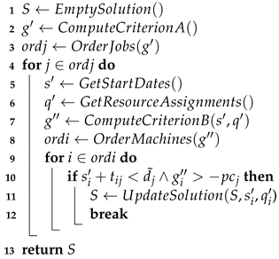
Algorithm 1 illustrates the constructive heuristic.    

Algorithm 1: Greedy constructive heuristic

    We begin by initializing the solution S. It is initially empty, with its elements ($STJ$, $FTJ$, $STM$, $FTM$, $STR$, $FTR$, $AMJ$, $ARJ$) set to 0, i.e., 0 starting and completion times for all jobs, machines, and resources, as well as no assignments of jobs to machines and resources.

We then compute a first criterion in order to evaluate each job (line 2 of Algorithm 1, called by function $ComputeCriterionA\left(\right)$). This criterion consists of two sub-criteria:

• Tardiness-related aspects;
• Cost-related aspects.

The first sub-criterion is given as:

$$\frac{t{c}_j}{d_j·t_j^{\prime }·m_j^{\prime }},\forall j\in 1\dots n$$

where $t_j^{\prime }$ is the average processing time of task j on all of the machines that can process it and $m_j^{\prime }$ is the number of such machines.

If we were to order tasks in decreasing order of this sub-criterion, we would give priority to tasks with a high tardiness cost, small due date, and small average processing time.

The second sub-criterion is given as:

$${\displaystyle p_j-f{c}_j-\sum _{r=1}^k{a}_{j}r·rc{r}_r·t_j^{\prime }+p{c}_j}$$

Ordering tasks in decreasing order of this sub-criterion gives priority to high-paying and high-penalty jobs.

We combine the two sub-criteria by normalizing the first and multiplying it with the second.

This first criterion is then used to sequence the jobs in decreasing order (line 3 of Algorithm 1).

For each job j in this order, we proceed to construct a sequence of machines to which it should be assigned. In order to construct this sequence, we first go through several steps.

We start by identifying the earliest starting date for job j on each machine i that can process it (line 5 of Algorithm 1):

$${\displaystyle s_i^{\prime }=max\left(trt{j}_{ij},FT{M}_i,\underset{r\in 1\dots k}{max}\left(a_{jr}·\underset{q\in 1\dots l_r}{min}\left(FT{R}_{rq}+trt{r}_{irq}^{\prime }\right)\right)\right),}$$

where

$$trt{r}_{irq}^{\prime }=\left\{\begin{array}{cc}trt{r}_r\hfill & {\displaystyle ,\mathrm{if}i\ne AM{J}_{j^{\prime }}\mathrm{where}{j}^{\prime }=\underset{\genfrac{}{}{0pt}{}{j^{″}\in 1\dots n}{AR{J}_{j^{″}r}=q}}{arg\; max}FT{J}_{j^{″}}}\hfill \\ 0\hfill & ,\mathrm{otherwise}\hfill \end{array}\right.$$

A job j will start on machine i no earlier that the time needed to transport it to the machine and the time the machine and the resources that it requires become available.

When estimating the availability time of resources, we consider all resources and use $a_{jr}$ to reduce this value to 0 if the resource type r is not required to process job j. For all needed resource types ($a_{jr}=1$), we estimate their available time and select the largest value, since they all need to be available throughout the duration of the job. For each resource type r, we look at all units of this resource ($q\in 1\dots l_r$) and select the one that would be available first using its complete date $FT{R}_{rq}$ and adding a transport time if this resource was last used on a different machine than i.

Estimating whether a transport time is required is carried out using $trt{r}_{irq}^{\prime }$. If the last task using resource q of type r is performed on a different machine than i, then a transport time is required; otherwise, this time is set to 0.

We also record the resource units that were selected when constructing $s^{\prime }$ using $q^{\prime }$ (line 6 of Algorithm 1):

$${\displaystyle q_{ir}^{\prime }=\underset{q\in 1\dots l_r}{arg\; min}(FT{R}_{rq}+trt{r}_{irq}^{\prime })}$$

Using $s^{\prime }$ and $q^{\prime }$, we then evaluate each machine i using a second criterion (line 7 of Algorithm 1, called by function $ComputeCriterionB(s^{\prime },q^{\prime })$), which is given as:

$${\displaystyle p_j-f{c}_j-trc{j}_{ij}-rc{m}_i·t_{ij}-irc{m}_i-\sum _{r=1}^k{a}_{jr}·(rc{r}_r·t_{ij}+irc{r}_{ir})-t{c}_j·max(0,s_i^{\prime }+t_{ij}-d_j),}$$

where

$$irc{m}_i=\left\{\begin{array}{cc}rc{m}_i·(s_i^{\prime }-FT{M}_i)\hfill & ,\mathrm{if}FT{M}_i>0\hfill \\ 0\hfill & ,\mathrm{otherwise}\hfill \end{array}\right.$$

$$irc{r}_{ir}=\left\{\begin{array}{cc}rc{r}_r·(s_i^{\prime }-FT{R}_{r{q}_{ir}^{\prime }})\hfill & ,\mathrm{if}FT{R}_{r{q}_{ir}^{\prime }}>0\hfill \\ 0\hfill & ,\mathrm{otherwise}\hfill \end{array}\right.$$

This criterion computes the net gain from selecting job j to be processed on machine i at time $s_i^{\prime }$ using its required resources $q_{ir}^{\prime },\forall r\in 1\dots k$. This criterion includes the selling price of the job ($p_j$), its fixed costs ($f{c}_j$), the cost of transporting the job to the machine ($trc{j}_{ij}$), the renting cost of the machine while executing the job ($rc{m}_i·t_{ij}$), the idle time of renting the machine if it was used to process other jobs ($irc{m}_i$), the renting cost of the required resources during the job processing but also during idle times for resources that have been used to process other jobs, and, finally, the tardiness costs.

Estimating the idle cost of machine i is carried out by checking whether $FT{M}_i$ is greater than 0, and, in this case, $irc{m}_i$ is equal to the cost of renting the machine per unit of time multiplied with the time between its latest complete date ($FT{M}_i$) and the estimated start date of job j ($s_i^{\prime }$).

Estimating the idle cost of a resource r ($irc{r}_{ir}$) is carried out in a similar way, considering the resource that should be selected in order to process job j.

Using the second criterion, we sequence the machines in decreasing order (line 8 of Algorithm 1). We then consider each machine from this list and select the first that does not lead the job to overshoot its deadline nor lead to a loss that is worse than if the job were not processed at all (line 10 of Algorithm 1). Once a machine fulfilling these conditions is found, we update the solution (line 11 of Algorithm 1) and jump to the next job (line 12 of Algorithm 1). If there is no machine that can fulfil these conditions, then the job is not processed.

3.2.2. Simulated Annealing

We consider a third heuristic for solving this problem: the simulated annealing procedure [35].

This approach starts from an initial solution and then moves to close neighbors across multiple iterations. During each iteration, the neighboring solution replaces the current one if it improves the objective function. Non-improving solutions may also replace the previous solution with a probability that is proportional to the performance difference and taking into account a temperature parameter. This parameters is initially set to a high value and decreases at each iteration. High values increase the probability of accepting non-improving solutions, and low values do not. Therefore, the approach starts by exploring the search space and ends by intensifying its search.

The performance of the simulated annealing approach is heavily dependent on the choice of the initial temperature and the rate at which it decreases, also called an annealing schedule. Usually, the annealing schedule requires a significantly time-consuming tuning phase in order for the approach to perform well on a new problem.

Variants of this approach, where the annealing schedule adapts and requires no tuning, have been proposed, and we therefore consider one such approach here. Namely, we focus on the adaptive annealing schedule known as modified LAM [36].

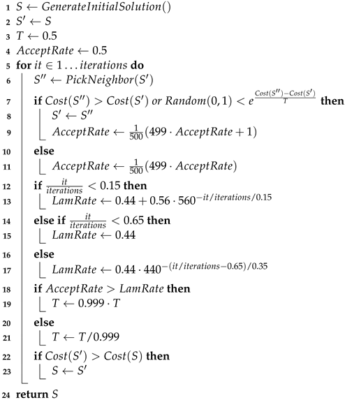
This adaptive simulated annealing (ASA) using the modified LAM annealing schedule is outlined in Algorithm 2.    

Algorithm 2: Adaptive simulated annealing using the modified LAM annealing schedule

The algorithm starts by initializing the solution S using the greedy constructive heuristic presented in Section 3.2.1 (line 1). A copy is also generated in the form of $S^{\prime }$ (line 2). The temperature parameter T and an $AcceptRate$ parameter are both set to $0.5$ (lines 3 and 4).

Throughout this algorithm, a solution of the problem is encoded using:

• $ordj$: the sequence of jobs;
• $AMJ$: the assignment of machines to jobs;
• $ARJ$: the assignment of resources to jobs.

For the initial solution, these elements correspond to those used by the constructive heuristic from Section 3.2.1. In order to evaluate a solution, a decoding function that generates all of the elements of the solution ($STJ$, $FTJ$, $STM$, $FTM$, $STR$, $FTR$, $AMJ$, $ARJ$) is used; however, for simplicity, we do not include these elements in the presentation of the algorithm. Initial values for the temperature and the acceptance rate are also set at this point.

We continue with the main loop of the algorithm (line 5 onward), which performs a preset number of iterations. Each iteration begins by generating a neighbor of solution $S^{\prime }$. In our case, generating a neighbor of $S^{\prime }$ consists of applying, with equal probability, one of the following operators:

• Swap two randomly selected jobs in $ordj$;
• Randomly change the machine assignment of one randomly selected job in $AMJ$;
• Randomly change the resource assignment of one randomly selected job in $AMJ$.

Once a neighbor $S^{″}$ is generated, it is accepted as the new solution and replaces $S^{\prime }$ if it is better or if a randomly selected value between 0 and 1 is lower than $e^{\frac{Cost\left(S^{″}\right)-Cost\left(S^{\prime }\right)}{T}}$ (lines 7 and 8). Otherwise, the same solution $S^{\prime }$ will be used during the next iteration.

The $AcceptRate$ and $LamRate$ parameters correspond to the modified LAM annealing schedule from [36], which the interested reader is referred to for further insight. Briefly speaking, this annealing schedule adapts the temperature so that the acceptance rate linearly decreases from 100% to 44% during the first 15% iterations of the algorithm, then fixes it at 44% during the following 50% iterations, while, for the remaining 35%, it drops linearly towards 0%.

4. Empirical Validation

In order to validate the algorithmic approaches for solving the presented problem, we devised a series of experiments.

4.1. Benchmark Generation

For a given problem size (n, m, and k are known), we built 20 instances where the problem parameters are generated as integer values using the following rules:

• $p_j\sim U(1000,10,000),\forall j\in 1\dots n$;
• $p{c}_j=\alpha ·p_j,\forall j\in 1\dots n$, where $\alpha \sim U(0.1,0.5)$;
• $f{c}_j=\beta ·(p_j-p{c}_j),\forall j\in 1\dots n$, where $\beta \sim U(0.2,0.5)$;
• $d_j\sim U(50,200),\forall j\in 1\dots n$;
• ${\tilde{d}}_j=\gamma ·d_j,\forall j\in 1\dots n$, where $\gamma \sim U(1,1.2)$;
• $t{c}_j\sim U(1,10),\forall j\in 1\dots n$;
• $rc{m}_i\sim U(10,50),\forall i\in 1\dots m$;
• $mwt{m}_i\sim U(10,100),\forall i\in 1\dots m$;
• $l_r\sim U(1,5),\forall r\in 1\dots k$;
• $rc{r}_r\sim U(10,50),\forall r\in 1\dots k$;
• $trc{r}_r\sim U(10,50),\forall r\in 1\dots k$;
• $trt{r}_r=\delta ·trc{r}_r$, where $\delta \sim U(0.1,0.3),\forall r\in 1\dots k$;
• $t_{ij}\sim U(5,50),\forall j\in 1\dots n,\forall i\in 1\dots m$;
• $trc{j}_{ij}\sim U(10,50),\forall j\in 1\dots n,\forall i\in 1\dots m$;
• $trt{j}_{ij}=\theta ·trc{j}_{ij}$, where $\theta \sim U(0.1,0.3),\forall j\in 1\dots n,\forall i\in 1\dots m$;
• $a_{jr}\sim U(0,1),\forall j\in 1\dots n,\forall r\in 1\dots k$.

When generating parameter a, we made sure that each resource type r is required by at least one job.

4.2. Experiments and Results

We present below the results from several numerical experiments using the exact and approximate approaches for solving the proposed scheduling problem. The experiments were conducted on an Intel Xeon Gold CPU with 80 cores at 2.00 GHz, and with 64 Gb RAM. All algorithms were implemented in julia 1.6.1 [37]. The MILP approach used the JuMP package and the the Gurobi 9.0.1 solver [38]. It was also allowed to use up to 16 cores and as much as 32 GB RAM, whereas, when executing each heuristic approach, we only used a single core.

We considered problem instances containing between 10 and 50 jobs (n), 10 and 20 machines (m), and 5 resource types (k). A total of 20 instances of each size were generated (all instances are available at github.com/aolteanu/UPMSP-NAJ-NAM-RR, accessed on 15 November 2022.) and tested, and the execution times were limited to 3600 seconds.

We begin by reporting the average gap and its standard deviation for all approaches in

Table 10. Gap from best solution in percentage (best results depicted in bold).

n	m	k	MILP		Greedy		SA (${10}^4$ iter.)		SA (${10}^5$ iter.)
			avg	std	avg	std	avg	std	avg	std
10	10	5	3	9	35	12	5	5	3	3
20	10	5	4	5	37	11	8	4	5	3
30	10	5	13	7	39	17	11	6	5	3
40	10	5	67	41	40	14	12	6	6	3
50	10	5	96	35	50	18	18	7	8	5
10	20	5	2	4	29	12	4	3	2	2
20	20	5	7	6	39	11	7	4	4	3
30	20	5	76	41	48	12	12	5	6	3
40	20	5	87	36	43	16	13	6	7	4
50	20	5	126	31	43	17	15	7	8	4

. The gap is given here by $\frac{best-actual}{best}$, where $actual$ is the objective value given by one algorithm execution on one problem instance, and $best$ is the best objective value found by any algorithm on that problem instance. The best average values are indicated in bold face.

We observe that, on small problem instances (10 and 20 jobs on 10 machines and 10 jobs on 20 machines), the MILP approach performs, as expected, better than most heuristic approaches. The simulated annealing approach with a large number of iterations, however, ties the MILP approach in the average gap value while also reporting a lower standard deviation. The MILP was, in fact, not able to prove the optimality of the solution, nor even find the best one for all problem instances within the allotted time. The performance of the MILP quickly degrades as the size of the problem instances grows, performing even worse than the greedy constructive heuristic.

Among the three tested heuristic approaches, the greedy constructive heuristic is consistently the worst performing, whereas the simulated annealing performs better, especially when increasing the number of iterations it performs. These remarks are also confirmed by the results from

Table 11. Number of best solutions found (best results depicted in bold).

n	m	k	MILP	Greedy	SA (${10}^4$ iter.)	SA (${10}^5$ iter.)
10	10	5	15	0	3	5
20	10	5	6	0	0	14
30	10	5	0	0	2	18
40	10	5	0	0	0	20
50	10	5	0	0	0	20
10	20	5	11	0	7	11
20	20	5	0	0	2	18
30	20	5	0	0	0	20
40	20	5	0	0	0	20
50	20	5	0	0	0	20

, where the MILP is able to find the best solutions for more problem instances when the number of jobs stays low ($n=10$); however, it gets quickly overtaken by the simulated annealing approach with ${10}^6$ iterations for $n>10$.

The execution times required for each tested approaches are illustrated in

Table 12. Execution time in seconds (best results depicted in bold).

n	m	k	MILP		Greedy		SA (${10}^4$ iter.)		SA (${10}^5$ iter.)
			avg	std	avg	std	avg	std	avg	std
10	10	5	3606	9	2	0	8	4	71	18
20	10	5	3612	9	2	0	11	4	106	19
30	10	5	3623	9	2	0	14	6	139	30
40	10	5	3638	10	2	0	18	6	162	26
50	10	5	3659	15	2	0	21	6	171	34
10	20	5	3612	9	2	0	8	4	72	17
20	20	5	3643	9	2	0	11	4	104	21
30	20	5	3720	26	2	0	15	4	136	33
40	20	5	3846	81	2	0	17	5	150	39
50	20	5	4130	238	2	0	22	6	176	35

.

We observe that the MILP always reaches its 3600-second time limit. Since, even for small-sized instances, it was not able to find the best solution overall, we conclude that more than one hour, or more computational resources, are needed for this approach. The constructive heuristic is the fastest, while the execution times of the simulated annealing are of the order of a few seconds when performing fewer iterations, and several minutes when performing more.

In order to evaluate the performance of the proposed approaches on instances of a more realistic size, we performed additional tests for problem instances with between 100 and 500 jobs, 50 machines, and 10 resource types.

Following the results from the smaller problem instances, we tested here only the heuristic approaches. We report the results on the gap and execution time in

Table 13. Gap from best solution in percentage and execution time (best results depicted in bold).

n	m	k	Gap				Execution Time
			Greedy		SA (${10}^4$ iter.)		Greedy		SA (${10}^4$ iter.)
			avg	std	avg	std	avg	std	avg	std
100	50	10	35	12	5	3	6	0	112	16
200	50	10	42	20	5	3	20	2	232	29
300	50	10	37	38	5	4	44	4	469	50
400	50	10	33	24	6	4	73	8	779	74
500	50	10	24	21	8	6	116	14	1202	107

.

We observe that the simulated annealing approach again performs the best, finding the best solution for each problem instance, although not for all of its 50 executions, as can be noticed from the average gap not being equal to 0. We can also conclude that the execution times for this approach remain reasonable for larger problem instances, which could be attributed to the increase in resource types ($k=10$), making it potentially easier to assign the needed resources when constructing a solution.

5. Conclusions and Perspectives

In this paper, a novel scheduling problem consisting of job and machine acceptance, the assignment of jobs to unrelated parallel machines, the scheduling of jobs on selected machines, and multiple-resource allocation was considered. The machines and renewable resources (such as manpower, industrial machines or tools, and computing devices) required for the processing of jobs were rented during their operating time. The objective was to maximize the overall profit. One practical application of the proposed problem consisted of establishing a production facility without (or with minimum) investment (in machinery and equipment) or location. Modeling existing infrastructure and manpower, in this case, can be easily achieved by reducing the renting costs and setup times to 0 for a given set of machines or resources. Another application corresponds to the illustrated event-planning problem.

In order to tackle this problem, we developed an exact approach based on mixed-integer linear programming as well as several heuristic approaches. Due to the complexity of the problem and following our experimental results, the exact approach may only be useful for smaller-sized problem instances. When larger, more realistic problem instances are considered, a self-adapting simulated annealing approach should be favored.

Additional work may consist of adapting the proposed approaches for other machine configurations, such as flowshop, or considering other real-world constraints, such as:

• Machine unavailability;
• Machine or resource renting discount based on the duration of their use;
• Resource transport duration dependent on machine and resource location;
• Ready times for jobs or resources;
• etc.