Joints Trajectory Planning of Robot Based on Slime Mould Whale Optimization Algorithm

Abstract

The joints running trajectory of a robot directly affects it’s working efficiency, stationarity and working quality. To solve the problems of slow convergence speed and weak global search ability in the current commonly used joint trajectory optimization algorithms, a joint trajectory planning method based on slime mould whale optimization algorithm (SMWOA) was researched, which could obtain the joint trajectory within a short time and with low energy consumption. On the basis of analyses of the whale optimization algorithm (WOA) and slime mould algorithm (SMA) in detail, the SMWOA was proposed by combining the two methods. By adjusting dynamic parameters and introducing dynamic weights, the proposed SMWOA increased the probability of obtaining the global optimal solution. The optimized results of 15 benchmark functions verified that the optimization accuracy of the SMWOA is clearly better than that of other classical algorithms. An experiment was carried out in which this algorithm was applied to joint trajectory optimization. Taking 6-DOF UR5 manipulator as an example, the results show that the optimized running time of the joints is reduced by 37.674% compared with that before optimization. The efficiency of robot joint motion was improved. This study provides a theoretical basis for the optimization of other engineering fields.

1. Introduction

With the development of the age, manufacturing has gradually become leaner in order to meet customer needs and ensure product quality. Zero-defect manufacturing (ZDM) [1] has become a new standard for manufacturing. More environmental protection, higher efficiency, and zero defects become the new requirements. In order to make product processing closer to ZDM, it is especially important to achieve the correct machining motion profile. Working accuracy and motion stationarity have become important indicators for the measurement of machining performance and have become research hotspots in the manufacturing industry. Legnani et al. [2] proposed a smooth interpolation method between any given angle pose by combining rotations and simple polynomials, with the duration of these different segments having the ability to be arbitrarily modified to optimize the trajectory. This method allows for attitude transition from any direction, which allows for a continuity of angular position, velocity and acceleration. The stationarity was improved in the machining process. Aggogeri et al. [3] built a combined feedback–feedforward adaptive regulator based on the concept of a harmonic steady-state. The vibration generated in the machining process was suppressed. Experiments on a four-axis machine tool showed that the proposed method could greatly reduce the vibration amplitude. Borboni et al. [4] analysed the influence of discretization truncation and interpolation on the ideal motion line. The numerical and experimental experiments demonstrated that linear interpolation was an effective interpolation method. Multiple points were interpolated in the optimal range so that excessive interpolation was avoided and better dynamic results were obtained. Incerti et al. [5] designed an operational approach to define a computational model that can simulate the dynamic behaviour of servomechanisms. The model had the characteristics of elasticity and backlash. Based on the typical control scheme of position feedback and a PID regulator, the computational module in the software could optimize and evaluate the dynamic performance of the servo mechanism in different experiments. The relevant parameters were calibrated. For joint robots commonly used in industry, the machining motion contour is presented in Cartesian space, and the accuracy of the machining motion contour depends on the trajectory of each joint in the joint space. Therefore, the research of joint trajectory planning is of great significance in obtaining a more accurate machining motion contour.

1.1. Literature Review

Trajectory planning works to solve the displacement, velocity and acceleration of each joint in real time according to the motion path and trajectory of the manipulator based on its task requirements, so as to generate a motion trajectory. When trajectory planning is carried out in joint space, a time function is generally used to describe joint variables and plan their first-order and second-order time derivatives [6]. It is therefore also called planning considering differential constraints. In general, the motion path points are first transformed into joint path points using inverse kinematics equations, and then smooth fitting is performed on each joint path point [7]. Commonly used trajectory planning interpolation algorithms include cubic polynomial, quintic polynomial, cubic B-spline, parabolic transition, mixed interpolation, etc. The cubic polynomial is simple to calculate, but it cannot guarantee continuous acceleration. Due to vibration and impact in the machining process it is a suitable algorithm for simple point-to-point motion. The quintic polynomial increases the acceleration constraint, which reduces the impact and increases the computation. It is suitable for high-speed and high-performance motion from point to point. The multi-segment polynomial interpolation algorithm is suitable for multi-point continuous motion, but the smoothness of the joints is not guaranteed. Spline curves with geometric invariance, local support and other characteristics can make multi-segment trajectory transitions smooth and reduce joint impact. In the Cartesian space, the joint-angles need to be obtained by solving the inverse kinematics equation many times, and angular velocities of the joints are obtained by solving the inverse of the Jacobian matrix [8].

For the optimal trajectory planning of manipulator joints, the current research focuses on optimization based on time, system energy and the presence of multiple objectives. For the study of time-optimal trajectory planning, Choi et al. [9] fused kinematic methods and evolutionary strategies for the trajectory planning of optimizers. This is effective for specific articulated robots for which it is difficult to obtain exact dynamics equations. Guo et al. [10] studied the planning of time-optimal trajectories of space robots under dynamical constraints based on particle swarm algorithms. Yin et al. [11] interpolated the position sequence of joints using cubic spline. An adaptive genetic algorithm that introduced the penalty function was used to optimize the shortest time trajectory. Lian [12] proposed a multi-variate time optimization method to optimize the trajectory of each joint based on a smooth trajectory generator. Yu et al. [13] combined a second-order continuous polynomial interpolation function with the optimization subject of a cosine reduced-weight particle swarm constrained by kinematics and dynamics. A time-optimal (TO) strategy was proposed and the motion time of the manipulator was successfully optimized. Cheng et al. [14] transformed the trajectory of a manipulator into a position and time series in the joint space by inverse kinematics. The quintic B-spline curve was used for interpolation. The objective function was optimized by the non-dominated sorting genetic algorithm (NSGA-II) and a time-optimal, safe, collision-free trajectory planning method was proposed. Yu et al. [15] designed a time-optimal trajectory planning method for robotic arms, which could search for optimal paths simultaneously. A uniform cubic b-spline interpolation algorithm was proposed to derive the motion curve expression of the manipulator joint with unknown path points. The trajectory was optimized based on the genetic algorithm. Zhao et al. [16] introduced chaos strategy and inertia weight to optimize the whale optimization algorithm and applied it to the trajectory planning of a robot arm. The Wolf optimization algorithm and particle swarm optimization (PSO) algorithm were compared. The improved algorithm is more accurate and is faster.

In terms of energy optimization, Hirakawa et al. [17] used B-spline curves and variational method to optimize the trajectory of redundant robots. Uarg et al. [18] combined a genetic algorithm and an adaptive simulated annealing algorithm. The minimum moment was set as the optimization objective for trajectory optimization. Cheng et al. [19] established a distributed dynamic physical model of a variable stiffness flexible robotic arm based on Hamilton’s theory. The minimum vibration displacement, minimum energy consumption, and minimum trajectory tracking deviation were taken as the performance objectives. The motion trajectory planning of the variable stiffness flexible robotic arm was carried out based on a cloud adaptive differential evolution (CADE) optimization algorithm.

For multi-objective optimization, Yang et al. [20] used the penalty function method to improve the objective function in the optimization process for the constraint problem. The improved objective function was solved by an improved genetic algorithm with elite strategy, and the diversity of the solution set was maintained. Different penalty costs for different levels of objective functions were significantly improved in terms of solution speed and efficiency. Based on the quintic non-uniform rational B-spline (NURBS) curve mathematician, taking the running time, energy consumption and trajectory pulsation as the objectives, Shi et al. used the non-dominated sorting genetic algorithm with an elitist strategy [21] (NSGA-II) and multi-objective particle swarm optimization algorithm [22] (MOPSO) to optimize the trajectory of industrial robots, respectively. The Pareto optimal solution set was obtained, and the normalized weight objective function was constructed to obtain a high-order continuous optimal trajectory. Feng et al. [23] fitted the trajectory of the robot joint space by the high-order polynomial interpolation method based on the particle swarm optimization algorithm to ensure the stability of the joint motion according to the kinematics characteristics of the robot. The algorithm structure is simple and easy to implement. Choubey et al. [24] achieved a fast convergence of error-free smooth continuous trajectories by the grey wolf optimization (GWO) method setting the tracking error, acceleration, etc. as the optimization objective. In the case of the consideration of multiple obstacles, taking time and energy consumption as optimization objectives, Fu et al. [25] used fourth- and the fifth-order polynomials as interpolation curves to fit the joint trajectory and an optimal trajectory under relevant constraints, based on a genetic algorithm, was obtained. Zhao et al. [26] constructed the trajectory of the manipulator in the joint space with the quintic B-spline interpolation method. An optimal objective function based on the time and average acceleration was then built and a hybrid optimization method of improved whale algorithm and particle swarm optimization (IWOA-PSO) was proposed. An effective time pulsation path planning algorithm was established. Vibration of the serial robot was reduced and working efficiency was improved. Setting the minimizing trajectory error, flight time and space as optimal objects, Gamze et al. [27] optimized the point-to-point motion planning in robot arm trajectory planning using non-dominated sorting genetic algorithm (NSGA-II), genetic algorithm (GA), artificial bee colony algorithm (ABC) and particle swarm optimization (PSO). The results were compared about the distance and time.

Through the above analysis, it can be seen that the trajectory planning of the manipulator is mainly in the form of a polynomial or spline curve. The commonly used trajectory optimization algorithms mainly include particle swarm optimization (PSO) algorithms, genetic algorithms (GA), whale optimization algorithms (WOA), etc. The forms used in joint trajectory optimization are summarized in

Table 1. Commonly used trajectory optimization algorithms.

Based Algorithm	Improved Algorithm	Interpolation Method
Particle swarm optimization (PSO)	PSO [10,23]	Quintic non-uniform rational B-spline curve (NURBS)
	Cosine reduced-weight PSO [13]	Cubic polynomial
	Multi-objective PSO (MOPSO) [22]	Quintic B-spline curve
Genetic algorithm (GA)	GA [15,25]	Cubic B-spline curve Fourth-fifth order polynomial
	Adaptive Genetic Algorithm [11]	Cubic spline interpolation
	Ranking Adaptive Genetic Algorithm (RAGA) [14]	Quintic B-spline curve
	Combining genetic algorithm and adaptive simulated annealing algorithm [18]	Cubic polynomial
	SUMTNSUA-II [20]	Quintic B-spline curve
	Non-dominated sorting genetic algorithm with elitist strategy (NSGA-II) [21]	Quintic B-spline curve
Whale optimization algorithm (WOA)	Improved WOA [16]	Quintic polynomial
	IWOA-PSO [26]	Quintic B-spline curve

. The PSO is widely used with simple structure and easily adjusted parameters. However, the convergence speed is slightly worse than that of GA. The related variants improved the optimization performance but made the calculation more complicated. A GA with short optimization time and high efficiency may improve the sudden change of angular acceleration, but the fixed parameters cannot meet the requirements of dynamic changes in the iterative process. It is easy to fall into local optimum. The WOA [28] has simple structure, few adjustment parameters and high optimization efficiency. The space information continues to be searched in subsequent iterations. The WOA has attracted the attention of many researchers with fewer operators, due to its characteristics that include an inclination to search, self-adaptation and self-learning. A series of improved algorithms have been proposed [29,30] and have been applied to optimization problems in many fields such as wireless sensor networks [31], solar cell design [32], DNA fragment assembly problem [33], etc. Based on this, this paper researched the optimization of the joint trajectory based on the WOA. Whereas, the algorithm and related variants still have problems, such as insufficient convergence and poor global search ability. Therefore, this paper improved the algorithm by fusion.

1.2. Contribution and Organization

The global search in the early stage and local search in the late stage of the WOA cannot jump out of the local optimal operation. Although the performance is excellent on simple problems, the optimization effect is unstable on complex problems. The slime mould optimization algorithm (SMA) [34] was proposed based on the diffusion and foraging behaviour of slime mould, which has the characteristics of fast convergence and strong optimization ability. In this paper, the WOA and SMA are fused, and the respective advantages of WOA and SMA algorithm are preserved. A hybrid whale slime mould optimization algorithm (SMWOA) is proposed, and the proposed algorithm is applied to the commonly used 6-DOF serial manipulator for joint trajectory optimization. The main innovations are as follows:

Change the value of a in WOA. The value of parameter a is replaced by that of the SMA, which can be dynamically adjusted with the advance of iteration times to adapt to the complex nonlinear search process.

The fitness weight ω is introduced. The fitness weight in SMA can adaptively adjust the distance between the current individual and the optimal individual. After its introduction into WOA, searching range and speed can be adaptively adjusted to strengthen the global search ability and accelerate the convergence speed.

The hybrid whale slime mould optimization algorithm (SMWOA) is proposed. The time optimal trajectory optimization of the six-joint manipulator is carried out with the cubic uniform B-spline interpolation method.

The rest of this article is organized as follows: Section 2 introduces the basic principles of WOA and SMA. The SMWOA is proposed and introduced in detail in Section 3. The process of joint trajectory optimization based on the SMWOA is introduced in Section 4 where the optimization results are analysed. Section 5 summarizes the content of this paper.

2. WOA and SMA

2.1. WOA

Mirjalili et al. [28] studied the bubble net predation method of humpback whales. A whale optimization algorithm (WOA) was proposed based on this spiral bubble net attack mechanism. Individual whales constantly update their positions to approach prey with different mechanisms, including encirclement, spiral bubble-net feeding manoeuvre and a global exploration phase. The mathematical model of the three parts is as follows.

(1)

Encircling prey

Suppose that the number of whale populations participating in the predation is N, and the dimension of the explored space is d. The position of the ith whale in the d-dimensional space at the tth iteration is expressed as:

$${\mathit{X}}_{nt}=(X_{n1},X_{n2},\dots ,X_{nd}),n=1,2,\dots ,N$$

(1)

The optimal position to date is denoted as the prey position, which is defined as:

$${\mathit{X}}^{\Delta }=(X_1^{\Delta },X_2^{\Delta },\dots ,X_d^{\Delta })$$

(2)

As the number of iterations increases, the optimal position is gradually updated and replaced. Because the initial population has no prior experience, whales initially choose random individual locations as their search targets. The process of searching and encircling prey can be expressed as:

$${\mathit{X}}_{n(t+1)}={\mathit{X}}_t^{\Delta }-\mathit{A}\cdot \mathit{D}$$

(3)

where A is the coefficient vector. D is the distance between the current individual and the current optimal individual, that is, the bounding step size, which is expressed as follows:

$$\{\begin{array}{l}\mathit{A}=2\mathit{a}\cdot {\mathit{r}}_{rand}-\mathit{a}\\ \mathit{D}=\left|2{\mathit{r}}_{rand}\cdot {\mathit{X}}_t^{\Delta }-{\mathit{X}}_t\right|\end{array}$$

(4)

where a is the convergence factor, whose element a = 2 − 2t/t_max, which decreases linearly from 2 to 0 as the number of iterations increases. r_rand is a random vector of [0, 1].

(2)

Spiral bubble-net feeding manoeuvre

When the humpback whales are swimming around the prey, they are also performing spiral motion predation. This behaviour is called spiral bubble-net predation. The mathematical model of this process can be expressed as:

$$\{\begin{array}{l}{\mathit{X}}_{n(t+1)}={\mathit{X}}_t^{\Delta }+{\mathit{D}}^{\prime }\cdot e^{bl}\cdot \cos (2\pi l)\\ {\mathit{D}}^{\prime }=\left|{\mathit{X}}_t^{\Delta }-{\mathit{X}}_t\right|\end{array}$$

(5)

where D’ is the distance between the current individual and the optimal individual in the tth iteration. b is the constant defining the logarithmic spiral shape. l is the random number between [−1,1].

Both mechanisms above belong to the development phase in the meta-heuristic optimization algorithm, in which the humpback whale keeps narrowing its range of movement and does spiral hunting at the same time. Assuming that the probability P of individual whales of two mechanisms is the same, that is, 50% for each, the mathematical model of these two approaches can be written as follows:

$$\{\begin{array}{l}{\mathit{X}}_{n(t+1)}={\mathit{X}}_t^{\Delta }-\mathit{A}\cdot \mathit{D}, P<0.5\\ {\mathit{X}}_{n(t+1)}={\mathit{X}}_t^{\Delta }+{\mathit{D}}^{\prime }\cdot e^{bl}\cdot \cos (2\pi l),P\ge 0.5\end{array}$$

(6)

(3)

Global exploration phase

This stage simulates the process that whale individuals search for food randomly according to mutual position. The mathematical model of this process can be expressed as Equation (7).

$$\{\begin{array}{l}{\mathit{X}}_{n(t+1)}={\mathit{X}}_t^r-\mathit{A}\cdot {\mathit{D}}^{″}\\ {\mathit{D}}^{″}=\left|2{\mathit{r}}_{rand}\cdot {\mathit{X}}_t^r-{\mathit{X}}_{nt}\right|\end{array}$$

(7)

where X_t^r is the whale individual position randomly selected. D″ are the distances between the current individual X_it and the random individual X_t^r in the tth iteration. The parameter vector A is consistent with the previous setting.

The choice of the above three predation mechanisms depends on the parameters P and A. If P ≥ 0.5, it directly enters the spiral bubble net predation mode. If P < 0.5, the whale individual is far away from the random individual and chooses to surround the prey when |A| < 1. The whale individual deviates from the prey and chooses the global random exploration mechanism to search for a better solution when |A| ≥ 1.

2.2. SMA

Slime mould can approach food according to the concentration of food odour in the air through slime mould veins. The stronger the food odour is, the stronger the biological oscillation wave is, the wider the slime mould veins are, and the more slime mould will gather in this area. On the contrary, when the food odour is weak, slime mould turns to explore other areas. The SMA algorithm is optimized by simulating the behavioural and morphological changes of mucilaginous vesicles during foraging. The algorithm calculates the weight of each position based on the merit of the fitness function of the current position and simulates the correlation between the morphological changes and contraction patterns of mucilaginous vesicles through the weight index.

The function expression is used to simulate the approximation behaviour. The search for the individual position X of the slime mould can be updated according to the best position of the X_B obtained so far. The updated equation of position is written as follows:

$${\mathit{X}}_{(t+1)}=\{\begin{array}{l}{r}_1\cdot (UB-LB)+LB,r_1<z\\ {\mathit{X}}^{\Delta }+{\mathit{v}}_{\mathit{b}}\cdot (\omega \cdot {\mathit{X}}_{At}-{\mathit{X}}_{Bt}),r_1\ge z\cup r_2<p\\ {\mathit{v}}_c\cdot {\mathit{X}}_t,r_1\ge z\cup r_2\ge p\end{array}$$

(8)

where r₁ and r₂ are random numbers from 0 to 1. UB and LB are the boundaries of the search range. X^Δ is the optimal position so far, that is, the highest position of food odour concentration. z is the probability factor of global search when surrounding food. X_At and X_Bt are two randomly selected slime mould locations. t represents the current number of iterations. v_c is the feedback factor, which describes the feedback relationship between food concentration and the quality of slime mould. This decreases linearly from 1 to 0. p is the control parameter, which is expressed as Equation (9):

$$p=\tanh \left|{\mathit{F}}_i-{\mathit{F}}^{\mathsf{\Delta }}\right|$$

(9)

where F_i is the fitness of the i-th individual in the current iteration, and F^Δ is the best fitness in all current iterations.

v_b is the vector parameter for [−a, a], and a is expressed as follows:

$$a=arc\tanh \left(-\raisebox{1ex}{$t$}\!\left/ \!\raisebox{-1ex}{$t_{\max }$}\right.+1\right)$$

(10)

ω represents the weight of slime mould, which can be written as follows:

$$\mathit{\omega }(\mathrm{sort}({\mathit{F}}_i))=\{\begin{array}{l}1+r\cdot \log (\frac{bF-F_i}{bF-wF}+1),Firsthalf\\ 1-r\cdot \log (\frac{bF-F_i}{bF-wF}+1),others\end{array}$$

(11)

where Firsthalf represents the species with F_i in the top half. bF represents the optimal fitness obtained in the current iteration process. wF is the worst fitness value obtained in the current iteration process. sort(F_i) represents the fitness sequence.

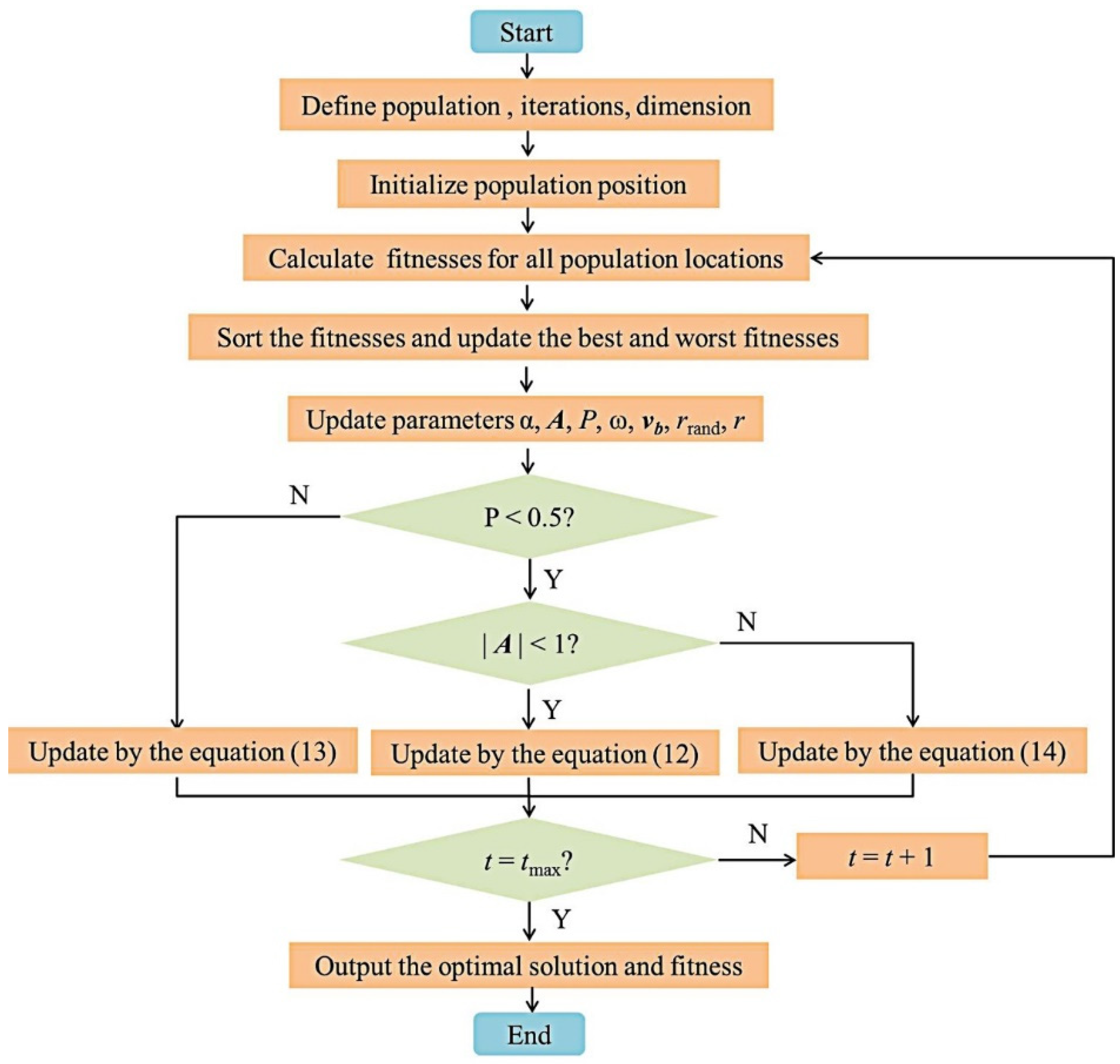
3. Slime Mould Whale Optimization Algorithm (SMWOA)

3.1. Principle of the SMWOA

This section describes the structure of the proposed SMWOA. In this algorithm, the mechanisms of SMA and WOA are combined to enhance the global optimization ability. The main fusion measures are as follows.

(1)

In WOA, parameter a decreases linearly from 2 to 0, and cannot accurately reflect and adapt to the complex nonlinear search process. Therefore, the expression of parameter a in SMA is used to replace parameter a in original WOA.

(2)

To improve the flexibility and diversity of the search domain, the fitness weight representing each slime mould individual is introduced into the position updating strategy of WOA, which is helpful in reaching the optimal value quickly.

The position iterative updating equations of encircling prey, spiral bubble-net feeding manoeuvre and global exploration phases after fusion are as follows:

$${\mathit{X}}_{n(t+1)}={\mathit{X}}_t^{\Delta }-\mathit{A}\cdot \mathit{D}$$

(12)

$${\mathit{X}}_{n(t+1)}={\mathit{X}}_t^{\Delta }+{\mathit{v}}_{\mathit{b}}\cdot e^{bl}\cdot \cos (2\pi l)\cdot {\mathit{D}}^{\prime }$$

(13)

$${\mathit{X}}_{n(t+1)}={\mathit{X}}_t^r-\mathit{A}\cdot {\mathit{D}}^{″}$$

(14)

The expressions of the parameters are as follows:

$$\{\begin{array}{l}\mathit{A}=2arc\tanh \left(-\raisebox{1ex}{$t$}\!\left/ \!\raisebox{-1ex}{$t_{\max }$}\right.+1\right)\cdot {\mathit{r}}_{rand}-arc\tanh \left(-\raisebox{1ex}{$t$}\!\left/ \!\raisebox{-1ex}{$t_{\max }$}\right.+1\right)\\ \mathit{D}=\left|2{\mathit{r}}_{rand}\cdot {\mathit{X}}_t^{\Delta }-{\mathit{X}}_t\right|\\ {\mathit{D}}^{\prime }=\left|\omega \cdot {\mathit{X}}_t^{\Delta }-{\mathit{X}}_t\right|\\ {\mathit{D}}^{″}=\left|\omega \cdot {\mathit{X}}_t^r-{\mathit{X}}_{nt}\right|\end{array}$$

(15)

The flow chart of the SMWOA is shown in Figure 1. Firstly, define the parameters of population and variables of the two algorithms, and create the initial population. Then, calculate and evaluate the fitness values of all individuals in the population. Compare and determine the optimal individual and the worst individual. The parameters are updated according to the corresponding equations. The Equation (13) is used to update the position when P ≥ 0.5. The Equation (12) is used to update the position when P < 0.5 and |A| < 1. The Equation (14) is used to update the position when P < 0.5 and |A| ≥ 1.

3.2. Computational Complexity

The computational complexity of the SMWOA mainly depends on the number of search agents, iterations and the location update mechanism. The SMWOA consists of initialization, fitness calculation ranking, weight update and position update. Suppose the number of search agents is N, the function dimension is d, and the maximum number of iterations is T. The computational complexity of initialization is ο(d). The computational complexity of fitness calculation and sorting is ο(N + N log N). The computational complexity of weight update is ο(N × d). The computational complexity of position update is ο(N × d). Therefore, the computational complexity of SMWOA is ο(d + T ∗ N ∗ (1 + log N + d)).

3.3. Performance Experiments of the SMWOA

Fifteen benchmark functions were selected as optimization objects in this paper to test the optimization effect of SMWOA, which are shown in

Table 2. Tested benchmark functions.

Functions	Expression	Dimension	Search Space	Optimal Value
Sphere	$F_1(x)={\displaystyle \sum _{k=1}^D{x}_k^2}$	30	[−100, 100]	0
Schwefel 2.22	$F_2(x)={\displaystyle \sum _{k=1}^D\left|x_k\right|}+{\displaystyle \prod _{k=1}^D\left|x_k\right|}$	30	[−10, 10]	0
Schwefel 1.12	$F_3(x)={{\displaystyle \sum _{k=1}^D\left({\displaystyle \sum _{l=1}^k{x}_l}\right)}}^2$	30	[−100, 100]	0
Schwefel 2.21	$F_4(x)=\underset{k}{\max }\left[\left|x_k\right|,1\le k\le D\right]$	30	[−100, 100]	0
Rosenbrock	$F_5(x)={\displaystyle \sum _{k=1}^{D-1}\left[100{((x_{k+1}-x_k^2))}^2+{(x_k-1)}^2\right]}$	30	[−30, 30]	0
Rastrigin	$F_6(x)={\displaystyle \sum _{k=1}^D\left[x_k^2-10\cos (2\pi x)+10\right]}$	30	[−5.12, 5.12]	0
Ackley	$\begin{array}{cc}\hfill F_7(x)=& -20\exp (-0.2\sqrt{\frac{1}{D}{\displaystyle \sum _{k=1}^D{x}_k^2}}-\exp (\frac{1}{D}{\displaystyle \sum _{k=1}^D\cos 2\pi x_k}))\hfill \\ & +20+e\hfill \end{array}$	30	[−32, 32]	0
Alpine	$F_8(x)={\displaystyle \sum _{k=1}^D\left|x_k\sin (x_k)+0.1x_k\right|}$		[−10, 10]	0
Penalized 1.1	$$\begin{gathered} \begin{array}{cc}{F}_9(x)=\hfill & \frac{\pi }{D}\cdot (10\sin (\pi y_1)+(y_k-1){}^2)+\hfill \\ & \frac{\pi }{D}\cdot {\displaystyle \sum _{k=1}^{D-1}{(y_k-1)}^2[1+10{\sin }^2(\pi y_{k+1})]}\hfill \\ & +{\displaystyle \sum _{k=1}^D\mu (x_k,10,100,4)}\hfill \end{array} \\ \begin{array}{cc}{y}_k=1+\frac{x_k+1}{4},\mu (x_k,p,a,m)=\{\begin{array}{l}p(x_k-a){}^m,x_k>a\\ 0,-a<x_k<a\\ p(-x_k-a){}^m,x_k<-a\end{array}\hfill & \end{array} \end{gathered}$$	30	[−50, 50]	0
Penalized 1.2	$\begin{array}{c}{F}_{10}(x)=0.1\{{\sin }^2(3\pi x_1)+{\displaystyle \sum _{k=1}^D{(x_k-1)}^2[1+{\sin }^2(3\pi x_k+1)]}+\\ {(x_k-1)}^2[1+{\sin }^2(2\pi x_k)]+{\displaystyle \sum _{k=1}^D\mu (x_k,5,100,4)}\}\end{array}$ $\mu (x_k,p,a,m)=\{\begin{array}{l}p(x_k-a){}^m,x_k>a\\ 0,-a<x_k<a\\ p(-x_k-a){}^m,x_k<-a\end{array}$	30	[−50, 50]	0
Michalewicz	$F_{11}(x)={(\frac{1}{500}+{\displaystyle \sum _{k=1}^{25}\frac{1}{l+{\displaystyle {\sum }_{k=1}^D(x_k-a_{kl})}}})}^{-1}$	2	[−65.536, 65.536]	1
Branin	$F_{12}(x)={(x_2-\frac{5.1}{4{\pi }^2}{x}_1^2+\frac{5}{\pi }{x}_1-6)}^2+10(1-\frac{1}{8\pi })\cos x_1+10$	2	[−5, 5]	0.398
Goldstein-Price	$\begin{array}{l}{F}_{13}(x)=[1+(x_1+x_2+1){}^2(19-14x_1+3x_1^2-14x_2+6x_1{x}_2+3x_2^2)]\\ \times [30+(2x_1-3x_2){}^2\times (18-32x_1+12x_1^2+48x_2-36x_1{x}_2+27x_2^2)]\end{array}$	2	[−2, 2]	3
Hartmann-3D	$F_{14}(x)=-{\displaystyle \sum _{k=1}^4{c}_k\exp }(-{\displaystyle \sum _{l=1}^3{a}_{kl}{(x_l-p_{kl})}^2})$	3	[0, 1]	−3.86
Shekel 5	$F_{15}(x)=-{\displaystyle \sum _{k=1}^5{[(X-a_k){(X-a_k)}^T{c}_k]}^{-1}}$	4	[0, 10]	−10.1532

. F1–F5 are unimodal functions. F6–F10 are multimodal functions. F11–F15 are fixed dimensional functions.

The experiments were carried out on an Intel(R) Core (TM) I5-6300HQ CPU @ 2.30 GHz Processor, 8 G RAM, MATL AB (2019b). The population size was set as 30, and the maximum number of iterations was 500. SMWOA was compared with algorithms WOA, SMA, PSO, DE and GSA. For each test function, all algorithms in the same dimension were independently run 30 times, and the average values and standard deviations were recorded. The Avg was used to test the convergence accuracy of the algorithm. The Std was used to test the stability. Wilcoxon rank sum test was carried out to verify the significant difference between the proposed algorithm and other algorithms. Comparison of optimization results is shown in

Table 3. Comparison of optimization results.

Functions	Evaluation Indexes	SMWOA	WOA	PSO	GSA	DE	SMA
F1	Avg	0.00 × 100	7.91 × 10−74	3.72 × 100	1.23 × 10−18	1.78 × 10−92	2.74 × 10−108
	Std	0.00 × 100	4.32 × 10−74	2.65 × 10−15	5.62 × 10−22	0.69 × 10−91	3.11 × 10−112
F2	Avg	3.57 × 10−67	1.86 × 10−49	2.05 × 10−1	6.46 × 10−10	3.09 × 10−1	3.75 × 10−24
	Std	2.51 × 10−64	2.39 × 10−48	1.52 × 10−1	0.00 × 100	2.78 × 10−1	2.89 × 10−26
F3	Avg	3.72 × 10−82	4.31 × 10−6	3.89 × 10−3	1.13 × 10−3	3.74 × 10−5	2.25 × 10−45
	Std	6.59 × 10−79	2.93 × 10−5	2.67 × 10−3	2.56 × 10−25	2.78 × 10−4	5.68 × 10−49
F4	Avg	2.58 × 10−16	7.25 × 10−12	4.56 × 10−8	7.86 × 10−10	3.72 × 10−14	2.74 × 10−23
	Std	3.67 × 10−15	3.97 × 10−12	3.28 × 10−9	3.57 × 10−9	2.88 × 10−13	3.11 × 10−26
F5	Avg	2.75 × 10−33	2.79 × 101	4.52 × 102	2.36 × 101	3.74 × 100	3.75 × 10−24
	Std	3.69 × 10−31	7.63 × 10−1	1.64 × 102	1.04 × 10−1	2.52 × 100	2.89 × 10−26
F6	Avg	5.04 × 10−29	1.06 × 10−21	1.29 × 102	2.32 × 101	5.27 × 10−3	0.00 × 100
	Std	6.52 × 10−30	2.39 × 10−21	3.64 × 101	7.85 × 10−18	6.43 × 10−6	0.00 × 100
F7	Avg	6.54 × 10−28	5.39 × 10−15	3.77 × 10−3	6.32 × 10−8	4.47 × 10−4	2.74 × 10−26
	Std	6.17 × 10−27	2.93 × 10−6	2.58 × 10−4	2.24 × 10−7	3.23 × 10−4	3.11 × 10−24
F8	Avg	6.24 × 10−39	1.26 × 10−2	5.79 × 10−1	3.58 × 100	3.78 × 10−2	3.75 × 10−24
	Std	2.63 × 10−39	3.97 × 10−1	2.35 × 10−3	2.79 × 10−1	9.01 × 10−1	2.89 × 10−26
F9	Avg	4.37 × 10−15	3.05 × 10−3	5.69 × 100	1.32 × 100	7.63 × 10−1	2.25 × 10−15
	Std	3.62 × 10−15	7.60 × 10−2	2.29 × 100	1.59 × 10−1	5.22 × 10−2	5.61 × 10−17
F10	Avg	2.47 × 10−10	8.97 × 100	3.74 × 100	5.22 × 10−1	3.24 × 10−1	2.74 × 10−8
	Std	3.64 × 10−11	6.69 × 100	2.28 × 100	5.32 × 10−1	2.56 × 100	3.11 × 10−9
F11	Avg	1.80 × 100	3.76 × 100	1.89 × 100	4.59 × 100	2.58 × 100	1.75 × 100
	Std	1.08 × 100	2.59 × 100	1.37 × 100	3.26 × 100	3.97 × 100	2.89 × 10−1
F12	Avg	0.42034	0.42718	0.41581	0.40278	0.39997	0.43669
	Std	2.55 × 10−3	3.97 × 10−1	2.25 × 10−2	4.14 × 10−3	6.32 × 10−5	5.12 × 100
F13	Avg	3.00007	3.001	3.0019	3.0007	3.0022	3.00011
	Std	1.36 × 10−4	7.62 × 10−1	1.39 × 100	2.67 × 10−2	2.63 × 101	1.05 × 10−3
F14	Avg	−3.8563	−3.8349	−3.8498	−3.8462	−3.8547	−3.8529
	Std	3.23 × 10−7	5.92 × 10−2	7.68 × 10−6	3.29 × 10−5	6.12 × 10−8	2.86 × 10−6
F15	Avg	−10.1337	−8.2895	−8.1933	−8.0774	−8.1324	−10.1024
	Std	3.24 × 10−3	2.73 × 100	4.63 × 100	4.89 × 100	5.79 × 101	1.41 × 10−2
p/h			8.24 × 10−6/+	4.37 × 10−7/+	2.16 × 10−7/+	3.12 × 10−6/+	1.38 × 10−5/+
Average ranking		1.4000	3.9333	5.1333	4.6000	3.8000	2.1333
Total rank		1	4	6	5	3	2

. In the tests of F1–F5 of the unimodal function method, all of them ranked first except F4. The unimodal function has only one global optimal value. The tests indicate that the SMWOA has strong mining ability. The multimodal functions F7, F8 and F10 rank first, while F6 and F9 rank second. The tests of multimodal functions show that the SMWOA has strong exploration ability. In the optimization of dimensional functions, although only F13 and F15 ranked first, other F11, F12 and F14 ranked second. These results verify that the algorithm has the ability to jump out of local optimum. At the same time, it can be seen that the results of some test functions are not ideal, and the algorithm can be modified in the parameter adjustment. Overall, the proposed SMWOA has the best optimization performance among the algorithms.

4. Trajectory Optimization of Joints Based on SMWOA

4.1. Path Interpolation of Joints

Path planning of joints is the process of generating the motion curves of each joint after giving the position, velocity, acceleration and other constraints of the starting point, end point and intermediate points. The process can be divided into point-to-point planning, continuous planning and multi-node planning between the two kinds of planning. Of these, multi-node planning is widely used. The common node interpolation methods include cubic polynomial, quintic polynomial, spline interpolation, etc. The use of low order polynomial spline interpolation can achieve smaller interpolation errors and avoid Runge phenomenon caused by higher order polynomial, so spline interpolation is used widely. The B spline curve has good qualities, such as geometrical invariability, convex hull and reduction of variation. The curve can be locally controlled and generated by the B spline curve. Therefore, this paper conducts interpolation based on cubic uniform B-spline curves [35], and its mathematical expression can be written as follows:

$${\theta }_i(u)={\displaystyle \sum _{j=0}^3{B}_{j,3}(u)V_{i+j-1}}$$

(16)

where θ_i(u) is the number of vectors at the ith point corresponding to the parameter u of spline curve, u ∈ [0, 1]. V_i+j−1 is the controlled point of the spline curve. B_j,3(u) is polynomial, that is,

$$\{\begin{array}{l}{B}_{0,3}(u)=\frac{-u^3+3u^2-3u+1}{6}\\ B_{1,3}(u)=\frac{3u^3-6u^2+4}{6}\\ B_{2,3}(u)=\frac{-3u^3+3u^2+3u+1}{6}\\ B_{3,3}(u)=\frac{u^3}{6}\end{array}$$

(17)

The Equation (16) can be rewritten in matrix form as:

$${\theta }_i(u)=\frac{1}{6}\left[\begin{array}{cccc}{u}^3& u^2& u& 1\end{array}\right]\left[\begin{array}{cccc}-1& 3& -3& 1\\ 3& -6& 3& 0\\ -3& 0& 3& 0\\ 1& 4& 1& 0\end{array}\right]\left[\begin{array}{c}{V}_{i-1}\\ V_i\\ V_{i+1}\\ V_{i+2}\end{array}\right]$$

(18)

To ensure the continuity of B-spline trajectories, the end vector of the former trajectory is equal to the first vector of the latter trajectory, that is,

$${\theta }_{i-1}(1)={\theta }_i(0)=\frac{1}{6}(V_{i-1}+4V_i+V_{i+1})=P_i(i=1,\dots ,n)$$

(19)

where P_i is the type of value point on a trajectory.

N equations can be determined by n type value points. Two boundary conditions are added as follows:

$$\{\begin{array}{c}{V}_0=V_1\\ V_n=V_{n+1}\end{array}$$

(20)

All the unknowns can be solved. The B spline curve determined by V_i−1, V_i, V_i+1, V_i+2 can be expressed as:

$$\begin{array}{l}\hfill {\theta }_i(u)=\frac{1}{6}(-u^3+3u^2-3u+1)V_{i-1}+\frac{1}{6}(3u^3-6u^2+4)V_i+\\ \hfill \frac{1}{6}(-3u^3+3u^2+3u+1)V_{i+1}+\frac{1}{6}{u}^3{V}_{i+2}(0\le u\le 1)\end{array}$$

(21)

The control point on the curve is defined as V_i (t_i, q_i). The joint angle change q(u) and time change t(u) of the ith segment trajectory on the curve are as follows respectively:

$$\{\begin{array}{c}t(u)=\frac{1}{6}\left[\begin{array}{cccc}{u}^3& u^2& u& 1\end{array}\right]\left[\begin{array}{cccc}-1& 3& -3& 1\\ 3& -6& 3& 0\\ -3& 0& 3& 0\\ 1& 4& 1& 0\end{array}\right]\left[\begin{array}{c}{t}_{i-1}\\ t_i\\ t_{i+1}\\ t_{i+2}\end{array}\right]\\ q(u)=\frac{1}{6}\left[\begin{array}{cccc}{u}^3& u^2& u& 1\end{array}\right]\left[\begin{array}{cccc}-1& 3& -3& 1\\ 3& -6& 3& 0\\ -3& 0& 3& 0\\ 1& 4& 1& 0\end{array}\right]\left[\begin{array}{c}{q}_{i-1}\\ q_i\\ q_{i+1}\\ q_{i+2}\end{array}\right]\end{array}$$

(22)

4.2. Objective Function and Constraint Function

The paper takes the time optimal, that is, the shortest movement time of the manipulator, as the objective function to optimize path. The mathematical model can be expressed as follows:

$$T=\min {\displaystyle \sum _{i=1}^{n-1}{h}_i}=\min {\displaystyle \sum _{i=1}^{n-1}(t_{i+1}-t_i)}$$

(23)

where h_i is the running time of each trajectory, and T is total time of the entire trajectory.

The velocity and acceleration of joints are constrained as follows:

(1) Constraint of velocity

Velocity expression of the manipulator joints can be obtained by taking the derivative of Equation (21).

$$\begin{array}{l}\hfill {\dot{\theta }}_i(u)=\frac{d}{du}{\theta }_i(u)=\frac{1}{2}(-u^2+2u-1)V_{i-1}+\frac{1}{2}(3u^2-4u)V_i\\ \hfill +\frac{1}{2}(-3u^2+2u+1)V_{i+1}+\frac{1}{2}{u}^2{V}_{i+2}(0\le u\le 1)\end{array}$$

(24)

This can be written with another form as Equation (25).

$${\dot{\theta }}_i(u)=\frac{d}{du}{\theta }_i(u)=\left[\frac{dt(u)}{du},\frac{dq(u)}{du}\right]=\left[t^{\prime },q^{\prime }\right]=\frac{q^{\prime }}{t^{\prime }}$$

(25)

(2) Constraint of acceleration

Acceleration expression ${\ddot{\theta }}_i(u)$ can be obtained by taking the derivative of Equation (24).

$$\begin{array}{l}\hfill {\ddot{\theta }}_i(u)=\frac{d}{du}{\dot{\theta }}_i(u)=\frac{1}{2}(-u^2+2u-1)V_{i-1}+\frac{1}{2}(3u^2-4u)V_i\\ \hfill +\frac{1}{2}(-3u^2+2u+1)V_{i+1}+\frac{1}{2}{u}^2{V}_{i+2}\end{array}$$

(26)

This can be written with another form as Equation (27).

$${\ddot{\theta }}_i(u)=\frac{d}{du}{\dot{\theta }}_i(u)=\left[\frac{d{t}^{\prime }(u)}{du},\frac{d{q}^{\prime }(u)}{du}\right]=\left[t^{″},q^{″}\right]=\frac{d{\dot{\theta }}_i(u)}{dt}=\frac{d{\dot{\theta }}_i(u)}{du}\frac{du}{dt}=\frac{q^{″}{t}^{\prime }-q^{\prime }{t}^{″}}{t^{\prime 3}}$$

(27)

The constraint functions of velocity and acceleration can be written as follows:

$$\{\begin{array}{l}{\dot{\theta }}_i(u)\le {\dot{\theta }}_{\max }\\ {\ddot{\theta }}_i(u)\le {\ddot{\theta }}_{\max }\end{array}$$

(28)

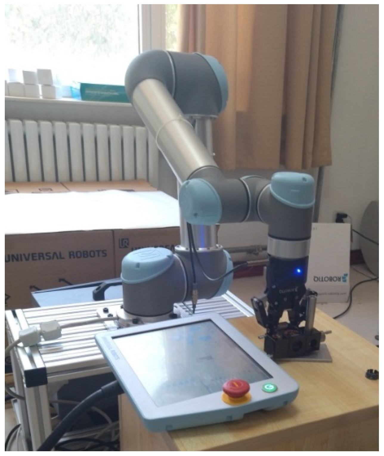
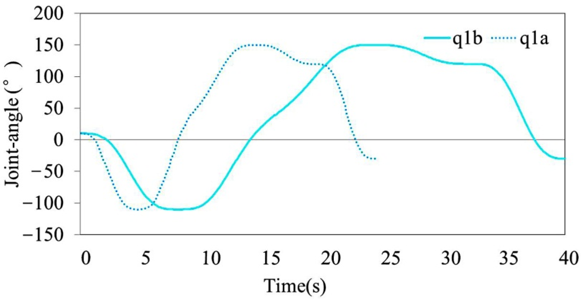
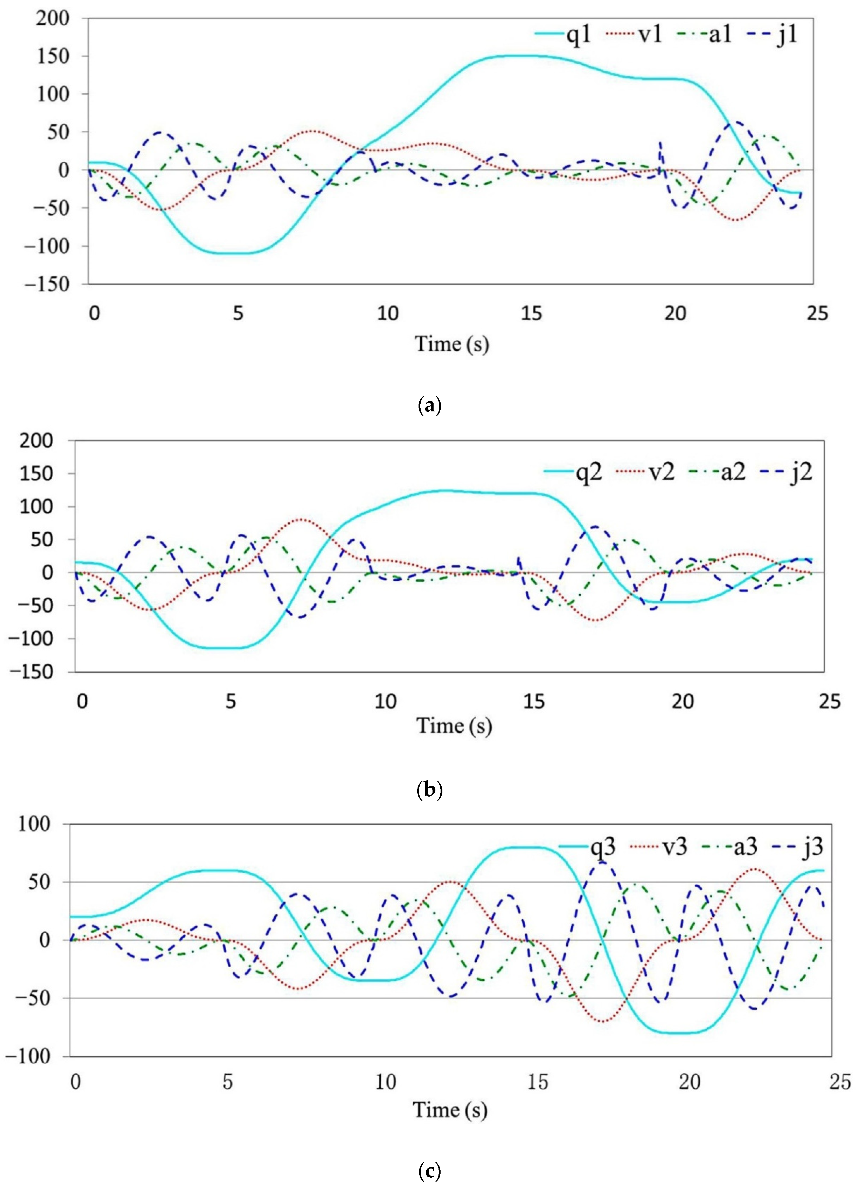
4.3. Optimal Experiment of Path Planning

The paper took a flexible and lightweight six-joint UR5 industrial robot developed by Universal Robots as the experimental platform, which is shown in Figure 2. The robot was equipped with a software system, control box, and visual programming control interface except manipulator. Users can program and adjust according to requirements.

To verify the optimal performance of the SMWOA on joints path planning, trajectory optimization of the UR5 manipulator was carried out taking the time as the optimal object. The position sequence of each joint is shown in

Table 4. Sequence of joint’s positions.

Nodes	Joints’ Positions
	θ1	θ2	θ3	θ4	θ5	θ6
1	10	15	20	5	10	6
2	−110	−115	60	50	−30	50
3	40	95	−35	180	75	80
4	150	120	80	100	−50	30
5	120	−45	-80	20	80	−80
6	−30	20	60	−60	50	100

. θ₁ is the angle of the base joint. θ₂ is the angle of the shoulder joint. θ₃ is the angle of the elbow joint. θ₄, θ₅ and θ₆ are all wrist joints.

The constraint values of each joint are shown in

Table 5. Constraints of joints.

Parameters	Constraints
	θ1	θ2	θ3	θ4	θ5	θ6
θmax (°)	320	250	270	280	200	300
${\dot{\theta }}_{\max }$ ((°)/s)	100	95	122	150	140	120
${\ddot{\theta }}_{max}$ ((°)/s2)	245	245	475	475	500	500

.

Population size was set as 100. The number of iterations was set as 100. The path of joints was optimized, and the comparison of time before and after optimization of base joint is shown in Figure 3. The abscissa is the running time of the joint path (s), and the ordinate is the angle-value of the base joint (°). The cyan thin solid line represents the trajectory curve of base joint before optimization, which is represented by q1b. The cyan dotted line represents the trajectory curve of base joint after optimization, which is represented by q1a. It can be seen in Figure 3 that the consumed time before optimization is 39.526 s. The optimized time is 24.635 s. The consumed time was reduced by 37.674%, and the operation efficiency of the manipulator was improved.

Angle, angular velocity, angular acceleration and angular jerk of joints after optimization are shown in Figure 4. Figure 4a represents the movement of base joint θ₁. Figure 4b represents the movement of shoulder joint θ₂. Figure 4c represents the movement of elbow joint θ₃. Figure 4d represents the movement of wrist joint θ₄. Figure 4e represents the movement of wrist joint θ₅. Figure 4f represents the movement of wrist joint θ₆. The horizontal coordinate refers to time, and the longitudinal coordinate refers to angle (°), angular velocity (°/s), angular acceleration (°/s²) and angular jerk (°/s³). The cyan thin solid line shows the change of the corresponding joint-angle, which is denoted by q_i (i = 1, 2, 3, 4, 5, 6). The red dot line represents the change of the corresponding joint- angular velocity, which is denoted by v_i. The green dash dot line represents the change of the corresponding joint-angular acceleration, which is denoted by a_i. The blue imaginary line shows the change of the corresponding joint-angular jerk, which is denoted by j_i. It can be seen that the optimized angular velocity and angular acceleration are in a gentle and stable state, and the angular jerk of joints θ₁, θ₂, θ₄ and θ₆ only appear as a cusp in the whole time range, with the remaining parts in a basically smooth state.

The proposed algorithm was compared with the SMA and WOA in the optimizing joint trajectory to verify the effectiveness of the SMWOA. The total time and spent time for each segment were recorded and compared, and the results are shown in

Table 6. Comparison of trajectory running time.

Algorithms	Time (s)					Total Time (s)
	h1	h2	h3	h4	h5
SMA	4.429	6.276	4.332	5.098	5.602	25.737
WOA	4.681	6.349	4.237	5.162	5.384	25.813
SMWOA	4.227	6.103	4.319	4.937	5.049	24.635

. The segment of trajectory from the ith node to the i+1th node is represented as h_i. The experimental results show that the optimization performance of the proposed SMWOA algorithm is superior to the SMA and WOA in joint trajectory planning.

5. Conclusions

To obtain the correct machining motion profile faster and make the machining quality closer to zero-defect manufacturing, this paper systematically investigated and researched the common optimized method of joints’ trajectories for the common series manipulator. To solve the problems of the current optimization algorithm, such as convergence insufficiency and poor global search ability, this paper proposed the slime mould whale optimization algorithm (SMWOA). The optimized characteristics of the commonly used WOA and SMA were analysed in detail. The advantages of the two methods were combined. The dynamic parameter a and dynamic weight ω of SMA were introduced into WOA and the SMWOA proposed. The optimized experiments of 15 benchmark functions were carried out, and the experiments verified that the optimization performance of the proposed algorithm was clearly better than that of other classical optimization algorithms. Taking the shortest running time as the optimized goal, the SMWOA algorithm was applied to the optimization of the joint trajectories of a serial manipulator. The experimental results also verified the effectiveness of the algorithm. Although the optimization performance of the proposed algorithm is better than other classical algorithms in the experimental tests in this paper, the optimization ability for high-dimensional functions and complex problems is still unclear. It can still be further improved in terms of parameter adjustment and search strategy.

References

1. Psarommatis, F.; May, G.; Dreyfus, P.A.; Kiritsis, D. Zero defect manufacturing: State-of-the-art review, shortcomings and future directions in research. Int. J. Prod. Res. 2020, 58, 1–17. [Google Scholar] [CrossRef]
2. Legnani, G.; Fassi, I.; Tasora, A.; Fusai, D. A practical algorithm for smooth interpolation between different angular positions. Mech. Mach. Theory 2021, 162, 104341. [Google Scholar] [CrossRef]
3. Aggogeri, F.; Merlo, A.; Pellegrini, N. Active Vibration Control Development in Ultra-Precision Machining. J. Vib. Control 2021, 27, 790–801. [Google Scholar] [CrossRef]
4. Borboni, A.; Aggogeri, F.; Elamvazuthi, I.; Incerti, G.; Magnani, P.L. Effects of profile interpolation in cam mechanisms. Mech. Mach. Theory 2020, 144, 103652. [Google Scholar] [CrossRef]
5. Incerti, G. Modeling and simulation of a position-controlled servo-axis with elasticity and backlash in the transmission. Arch. Appl. Mech. 2017, 87, 633–645. [Google Scholar] [CrossRef]
6. Liu, Z. Research and Simulation of Six-axis Industrial Robot Trajectory Planning Based on Robotics Toolbox. Mech. Eng. Autom. 2017, 3, 59–61. [Google Scholar]
7. Rossi, C.; Savino, S. Robot trajectory planning by assigning positions and tangential velocities. Robot. Comput.-Integr. Manuf. 2013, 29, 139–156. [Google Scholar] [CrossRef]
8. Wang, N.; Zhang, X. Trajectory planning and simulation of six-DOF robot based on MATLAB. Manuf. Autom. 2014, 15, 95–97. [Google Scholar]
9. Choi, T.; Park, C.; Do, H.; Park, D.; Kyung, J.; Chung, G. Trajectory correction based on shape peculiarity in direct teaching manipulator. Int. J. Control Autom. Syst. 2013, 11, 1009–1017. [Google Scholar] [CrossRef]
10. Guo, T.Y.; Li, F.; Huang, K.; Zhang, F.Z.; Feng, Q. Application of Optimal Algorithm on Trajectory Planning of Mechanical Arm Based on B Spline Curve. In Applied Mechanic and Materials; Trans Tech Publications Ltd.: Zurich, Switzerland, 2013; Volume 376, pp. 253–256. [Google Scholar]
11. Yin, F.; Liang, Q.; Cheng, X.; Tao, Z. Research on Mechanical Arm Joint Space Trajectory Planning Algorithm Based on Optimal Time. Mach. Des. Res. 2017, 33, 12–15. [Google Scholar]
12. Lian, L. Robot Joint Trajectory Planning Method Based on the Optimal Execution Time. Modul. Mach. Tool Autom. Manuf. Tech. 2018, 9, 57–60. [Google Scholar]
13. Yang, Y.; Xu, H.; Li, S.; Zhang, L.; Yao, X. Time-optimal trajectory optimization of serial robotic manipulator with kinematic and dynamic limits based on improved particle swarm optimization. Int. J. Adv. Manuf. Technol. 2022, 120, 1253–1264. [Google Scholar] [CrossRef]
14. Cheng, Q.; Hao, X.; Wang, Y.; Xu, W.; Li, S. Trajectory planning of transcranial magnetic stimulation manipulator based on time-safety collision optimization. Robot. Auton. Syst. 2022, 152, 104039. [Google Scholar] [CrossRef]
15. Yu, X.; Dong, M.; Yin, W. Time-optimal trajectory planning of manipulator with simultaneously searching the optimal path. Comput. Commun. 2022, 181, 446–453. [Google Scholar] [CrossRef]
16. Jing, Z.; Xijing, Z.; Xiaoling, M.; Xiao, W. Application of Improved Whale Optimization Algorithm in Time-Optimal Trajectory Planning of Manipulator. 2021. Available online: https://kns.cnki.net/kcms/detail/detail.aspx?doi=10.13433/j.cnki.1003-8728.20200596 (accessed on 21 October 2021). [CrossRef]
17. Hirakawa, A.R.; Kawamura, A. Trajectory generation for redundant manipulators under optimization of consumed electrical energy. In Proceedings of the Conference Record-IAS Annual Meeting (IEEE Industry Applications Society), San Diego, CA, USA, 6–10 October 1996; Volume 3, pp. 1626–1632. [Google Scholar]
18. Uarg, D.P.; Kumar, M. Camera calibration and sensor fusion in an automated flexible manufacturing multi robot work cell. Proc. Am. Control Conf. 2002, 6, 4934–4939. [Google Scholar]
19. Cheng, Q.; Xu, W.; Liu, Z.; Hao, X.; Wang, Y. Optimal Trajectory Planning of the Variable-Stiffness Flexible Manipulator Based on CADE Algorithm for Vibration Reduction Control. Front. Bioeng. Biotechnol. 2021, 9, 766495. [Google Scholar] [CrossRef]
20. Yang, Y.; Zhou, C.; Wang, W.; Peng, B. Multi-objective trajectory planning based on SUMTNSGA-II. Comput. Eng. Des. 2015, 36, 3076–3081. [Google Scholar]
21. Shi, X.; Fang, H.; Guo, W. Time-Energy-Jerk Optimal Trajectory Planning of Manipulators Based on Quintic NURBS. Mach. Des. Res. 2017, 33, 12–16. [Google Scholar]
22. Shi, X.; Fang, H. Time-Energy-Jerk Optimal Planning of Industrial Robot Trajectories. Mach. Des. Manuf. 2018, 6, 254–257. [Google Scholar]
23. Feng, B.; Liu, F.; Zheng, L. Optimal Motion Trajectory Planning of Robot Joint Space Based on Particle Swarm Optimization. Modul. Mach. Tool Autom. Manuf. Tech. 2018, 5, 1–4. [Google Scholar]
24. Choubey, C.; Ohri, J. Optimal Trajectory Generation for a 6-DOF Parallel Manipulator Using Grey Wolf Optimization Algorithm. Robotica 2021, 39, 411–427. [Google Scholar] [CrossRef]
25. Fu, Q.; Song, Y.; Wei, S.; Guo, L. Design of a kind of trajectory optimization algorithm for a manipulator based on genetic algorithm. Lect. Notes Electr. Eng. 2019, 529, 683–692. [Google Scholar]
26. Zhao, J.; Zhu, X.; Song, T. Serial Manipulator Time-Jerk Optimal Trajectory Planning Based on Hybrid IWOA-PSO Algorithm. IEEE Access 2022, 10, 6592–6604. [Google Scholar] [CrossRef]
27. Demir, G.; Vural, R.A. Heuristic Trajectory Planning of Robot Manipulator. In Proceedings of the 2021 IEEE Jordan International Joint Conference on Electrical Engineering and Information Technology (JEEIT), Amman, Jordan, 16–18 November 2021; pp. 222–226. [Google Scholar]
28. Mirjalili, S.; Lewis, A. The whale optimization algorithm. Adv. Eng. Softw. 2016, 95, 51–67. [Google Scholar] [CrossRef]
29. AbdelAziz, A.M.; Soliman, T.H.A.; Ghany, K.K.A.; Sewisy, A.A.E.M. A Pareto-Based Hybrid Whale Optimization Algorithm with Tabu Search for Multi-Objective Optimization. Algorithms 2019, 12, 261. [Google Scholar] [CrossRef]
30. Ghoniem, R.M.; Alhelwa, N.; Shaalan, K. A Novel Hybrid Genetic-Whale Optimization Model for Ontology Learning from Arabic Text. Algorithms 2019, 12, 182. [Google Scholar] [CrossRef]
31. Kotary, D.K.; Nanda, S.J.; Gupta, R. A many-objective whale optimization algorithm to perform robust distributed clustering in wireless sensor network. Appl. Soft Comput. 2021, 110, 107650. [Google Scholar] [CrossRef]
32. Elaziza, M.A.; Oliva, D. Parameter estimation of solar cells diode models by an improved opposition-based whale optimization algorithm. Energy Convers. Manag. 2018, 17, 1843–1859. [Google Scholar] [CrossRef]
33. Mohamed, A.B.; Reda, M.; Karam, M.S.; Ripon, K.C.; Michael, J.R. An Efficient-Assembler Whale Optimization Algorithm for DNA Fragment Assembly Problem: Analysis and Validations. IEEE Access 2020, 8, 222144–222167. [Google Scholar] [CrossRef]
34. Li, S.; Chen, H.; Wang, M.; Heidari, A.A.; Mirjalili, S. Slime mould algorithm: A new method for stochastic optimization. Future Gener. Comput. Syst. 2020, 111, 300–323. [Google Scholar] [CrossRef]
35. Sun, Y.; Yang, X.; Dai, R.; Chen, X.; Tan, S.; Xue, P. Kinematics Analysis and Palletizing Trajectory Planning of 6-DOF Robot. Mach. Tool Hydraul. 2021, 49, 33–37. [Google Scholar]
Figure 1. Flow chart of the SMWOA.
Algorithms 15 00363 g001
Figure 2. UR5 experimental platform.
Algorithms 15 00363 g002
Figure 3. Comparison before and after optimization.
Algorithms 15 00363 g003
Figure 4. Movements of joints after optimization based on the SMWOA. (a) Movement of base joint θ1; (b) Movement of shoulder joint θ2; (c) Movement of elbow joint θ3; (d) Movement of wrist joint θ4; (e) Movement of wrist joint θ5; (f) Movement of wrist joint θ6.
Algorithms 15 00363 g004aAlgorithms 15 00363 g004b