Foremost Walks and Paths in Interval Temporal Graphs ^†

Abstract

The min-wait foremost, min-hop foremost and min-cost foremost paths and walks problems in interval temporal graphs are considered. We prove that finding min-wait foremost and min-cost foremost walks and paths in interval temporal graphs is NP-hard. We develop a polynomial time algorithm for the single-source all-destinations min-hop foremost paths problem and a pseudopolynomial time algorithm for the single-source all-destinations min-wait foremost walks problem in interval temporal graphs. We benchmark our algorithms against algorithms presented by Bentert et al. for contact sequence graphs and show, experimentally, that our algorithms perform up to 207.5 times faster for finding min-hop foremost paths and up to 23.3 times faster for finding min-wait foremost walks.

1. Introduction

Temporal graphs are graphs in which the edges connecting vertices or the characteristics of these edges may change with time. The applications of temporal graphs include the spread of viral diseases, information dissemination by means of physical/virtual contact between people, understanding behavior in online social networks, modeling data transmission in phone networks, modeling traffic flow in road networks, and studying biological networks at the molecular level [1,2,3,4,5,6,7].

Two popular categories of temporal or dynamic graphs are contact-sequence (temporal) graphs and interval-temporal graphs. In a contact-sequence graph, each directed edge $(u,v)$ has the label $(departure\_time,travel\_duration)$, where $departure\_time$ is the time at which one can leave vertex u along edge $(u,v)$ and $travel\_duration$ is the time it takes to traverse the edge. Therefore, vertex v is reached at time $departure\_time+travel\_time$. Note that a contact-sequence graph may have many edges from vertex u to vertex v; each edge has a different $departure\_time$. In an interval-temporal graph, each directed edge $(u,v)$ has a label that is comprised of one or more tuples of the form $(start\_time,end\_time,travel\_duration)$, where $start\_time\le end\_time$ defines an interval of times at which one can depart vertex u. If one departs u at time t, $start\_time\le t\le end\_time$, one reaches v at time $t+travel\_duration$. The intervals associated with the possibly many tuples that comprise the label of an edge $(u,v)$ must be disjoint. Figure 1 and Figure 2 are examples of contact-sequence and interval-temporal graphs, respectively. A (time-respecting) $walk$ in a temporal graph is a sequence of edges with the property that the end vertex of one edge is the start vertex of the next edge (if any) on the walk, each edge is labeled by the departure time from the start vertex of the edge, and the departure time label on each edge is a valid departure time for that edge and is greater than or equal to the arrival time (if any) at the edge’s start vertex (A more formal definition is provided in Section 2). A (time-respecting) $path$ is a walk in which no vertex is repeated (i.e., there is no cycle). $<S,1,A,2,B>$ and $<S,0,B,5,C>$ are example walks in the temporal graphs of Figure 1 and Figure 2, respectively. Both walks are also paths.

An application that can be modeled with a contact-sequence graph is a flight network. Each flight has a departure time at which it leaves the originating airport and a certain travel duration before it can reach the destination airport. On the other hand, if we consider the example of a road network, there is no single instance of time when one needs to depart on a given street. There may be different time windows (or time intervals) during which a street may be open for travel. Further, we may define time windows based on travel duration needed to reach from point A to point B on a given street due to different traffic conditions during different times of the day (such as office hours). Such networks cannot be modeled using contact-sequence graphs, as a given time window represents infinitely many possible departure times and, hence, infinitely many contact sequence edges. It is easy to see that every contact-sequence graph can be modeled as an interval-temporal graph. Further, when time can be discretized, every interval-temporal graph can be modeled as a contact-sequence graph (with potentially an explosion in the number of edges).

The authors of [8,9,10,11] focus on finding optimal paths and walks. Optimization criteria such as $foremost$ (arrive at the destination at the earliest possible time), $minhop$ (use the fewest number of hops when going from the source to the destination vertex), $shortest$ (the time taken to go from the source to the destination is minimized), and so on, are considered. Gheibi et al. [12] present a new data structure for contact-sequence graphs that results in faster algorithms for many of the path problems studied in [8]. While [9] focuses on interval-temporal graphs, refs. [8,10] use the contact-sequence model. Ref. [10] presents an algorithm for finding walks that optimize any linear combination of eight different optimization criteria ($foremost,reverse\_foremost,fastest,shortest,$ $cheapest,most\_likely,min\_hop,min\_wait$). In our earlier paper [13], we developed algorithms to find optimal foremost and min-hop paths in interval-temporal graphs. These algorithms were demonstrated experimentally to run faster than earlier algorithms for these problems.

A temporal graph may have many walks/paths that optimize a criterion such as foremost. In some applications, it is required to find a walk/path that optimizes a secondary criterion from among all walks/paths that optimize a primary criterion. For example, we may desire a min-wait foremost path (i.e., a foremost path in which the sum of the wait times at intermediate vertices is minimized) or a min-hop foremost path (a foremost path that goes through the fewest number of edges). For example, when selecting flights to go from A to B one may wish to use a min-wait foremost path (a route that minimizes the total wait time at intermediate airports while getting to the destination at the earliest possible time) or a min-hop foremost path (a route that involves the fewest number of connections while guaranteeing the earliest possible arrival time). In this paper, we examine the min-wait, min-hop, and min-cost (each edge or edge interval has an additional attribute, its cost), foremost walks/paths problems.

As discussed in Section 6, the algorithm by Bentert et al. can be tuned by carefully choosing the coefficients for different optimization criteria to find min-hop foremost paths and min-wait foremost walks in contact-sequence temporal graphs. We use this method to benchmark our algorithms against the algorithm by Bentert et al. and show that we perform about 207.5 times faster for finding min-hop foremost paths and up to 23.3 times faster for finding min-wait foremost walks. Further, we solve these problems on the interval-temporal graphs that can represent a wider problem space for temporal graphs, as opposed to the contact-sequence temporal graphs.

Our main contributions in this paper are:

• We show that the problems for finding min-cost foremost and min-wait foremost paths and walks in interval temporal graphs are NP-hard.
• We develop a polynomial time algorithm for the single-source all-destinations min-hop foremost paths problem in interval-temporal graphs.
• We develop a pseudopolynomial time algorithm for the single-source all-destinations min-wait foremost walks problem in interval-temporal graphs.
• We show that the problem of finding min-hop foremost paths and min-wait foremost walks can be modeled using the linear combination formulation employed in Section 6 when the optimization criteria are discrete (e.g., time is discrete). Our modeling methodology readily extends to other primary and secondary criteria as well as to multiple levels of secondary criteria (e.g., shortest min-hop foremost path).
• We benchmark our algorithms against the algorithm of Bentert et al. [10] using datasets for which the preceding modeling can be used. On these datasets, our algorithm is up to 207.5 times faster for finding min-hop foremost paths and up to 23.3 faster for finding min-wait foremost walks.

The roadmap of this paper is as follows. In Section 2, we describe the problems of finding min-hop foremost paths ($mhf$ paths), min-wait foremost walks ($mwf$ walks), and min-cost foremost paths ($mcf$ paths). In Section 3, we show that the problems of finding $mwf$ paths and walks and the problem for finding $mcf$ paths in interval temporal graphs are NP-hard. In Section 4, we present theorems that describe the properties of min-hop foremost paths in temporal graphs. We review the data structures used to represent interval-temporal graphs along with some fundamental functions necessary for the algorithm for finding $mhf$ paths. Finally, we present the algorithm for finding $mhf$ paths in interval-temporal graphs along with the proof of its correctness and its computational complexity. In Section 5, we present theorems that describe the properties of $mwf$ walks in interval-temporal graphs. We introduce additional data structures required by the algorithm we propose for finding $mwf$ walks in interval-temporal graphs. Finally, we present the algorithm for finding the $mwf$ walks in interval-temporal graphs along with proof of its correctness and complexity analysis. In Section 6, we show how the problems for finding foremost paths and walks with a secondary optimization criteria can be modeled as optimal walks with linear combination of multiple optimization criteria. We use this modeling to find $mhf$ paths and $mwf$ walks in contact sequence graphs using the algorithm of Bentert et al. [10], which optimizes a linear combination of criteria. In Section 7, we compare our algorithms for finding $mhf$ paths and $mwf$ walks with the algorithm by Bentert et al. [10] by transforming contact-sequence graphs to interval-temporal graphs and vice versa. Finally, we conclude in Section 8.

2. Foremost Walks and Paths

A $walk$ (equivalently, valid walk, temporal walk or time-respecting walk) in a temporal graph is an alternating sequence of vertices and departure times $u_{t0},t_0,u_{t1},t_1,...,u_{tk}$ where (a) $t_i$ is a permissible departure time from $u_{ti}$ to $u_{t_{i+1}}$ and (b) for $0\le i<k-1$, $t_i+{\mathsf{\lambda }}_i)\le t_{i+1}$. Here, ${\mathsf{\lambda }}_i$ is the travel duration when departing $u_{ti}$ at $t_i$ using the edge $(u_{ti},u_{t_{i+1}})$ (i.e., $t_i+{\mathsf{\lambda }}_i$ is the arrival time at $u_{t_{i+1}}$). For this $walk$, $u_{t0}$ is the source vertex and $u_{tk}$ the destination. Note that every walk in which a vertex is repeated contains one or more cycles. A walk that has no cycle (equivalently, no vertex repeats) is a path.

$W_1=S,0,B,5,C$ is a walk from S to C in the temporal graph of Figure 2. $W_2=S,0,A,1,B,3,C,5,A$ is another walk in the temporal graph of Figure 2. $W_1$ does not contain any cycles as none of the vertices are repeated from source to destination. Hence, $W_1$ is also a path. However, $W_2$ has vertex A that repeats. Therefore, it is not a path. We are interested in $foremost$ paths and walks in a temporal graph that start at a vertex s at a time $\ge t_{start}$ and end at another vertex v. As defined in [8,9,10], a $foremost$ walk is a walk from a source vertex s to a destination vertex v that starts at or after a given time $t_{start}$ and has the arrival time $t_f$, which is the earliest possible arrival time at the destination v among all possible walks from s to v.

2.1. Min-Hop Foremost

A min-Hop foremost ($mhf$) walk is a foremost walk from a source vertex s to another vertex v that goes through the fewest number of intermediate vertices. We observe that every $mhf$ walk is an $mhf$ path, as cycles may be removed from any s to v walk to obtain a path with a fewer number of hops and the same arrival time at v. For this reason, we refer to $mhf$ walks as $mhf$ paths in the rest of this paper.

As an example, consider the interval-temporal graph of Figure 3. Every walk in this graph is also a path. The paths $P1=<a,0,b,1,c,7,d>$ and $P2=<a,0,c,7,d>$ arrive at d at time 8 and are foremost paths from a to d. $P2$ is a 2-hop foremost path while $P1$ is a 3-hop foremost path. $P2$ is the only min-hop foremost path or $mhf$ path from a to d in Figure 3.

2.2. Min-Wait Foremost

A min-wait foremost or $mwf$ walk is a $foremost$ walk from a source vertex s to any other vertex v that accumulates minimum total wait time at the vertices visited by the walk. The wait time at each vertex u is $departure\_time\left(u\right)-arrival\_time\left(u\right)$. The total wait time accumulated by the walk is the sum of the wait times at each vertex u. Therefore, $mwf$ walk is a foremost walk from s to v that minimizes $({\sum }_{u_{ti}}departure\_time\left(u_{ti}\right)-arrival\_time\left(u_{ti}\right))$ where $u_{ti}\in vertices\left(mwf(s,v)\right)$ and $u_{ti}\ne s;u_{ti}\ne v$, as there is no wait time accumulated at the source vertex and the destination vertex.

$mwf$ walks can have cycles, as is evident from the example of Figure 4. The $mwf$ walk from source vertex s to destination vertex b is $mwf(s,b)=s,0,a,2,c,4,d,5,a,7,b$, arriving at b at time 8 with total wait time of 1 accumulated at vertex a. Alternate $foremost$ paths from s to b are $P1=s,0,a,4,b$, arriving at time 8 with a wait time of 3, and $P2=s,0,a,7,b$, also arriving at 8 with a wait time of 6. Therefore, to reduce the total wait time along the walk, we may need to go through cycles instead of waiting for a long time at a given vertex.

2.3. Min-Cost Foremost

For this problem, we assume there is a non-negative cost associated with every edge traveled along the walk from source vertex s to a destination vertex v. The cost of an edge may depend on the departure time from the edge’s start vertex. The min-cost foremost or $mcf$ walk is a foremost walk from source vertex s to any other vertex v that incurs minimum cost along the walk. The cost incurred on a time arc from a vertex $u_{ti}$ to $u_{ti+1}$ departing at time $t_i$ is denoted by a function $c(u_{ti},u_{ti+1})$. Therefore, the objective for the min-cost foremost or $mcf$ walk problem is to find a walk from a given source vertex s to a destination vertex v with the arrival time $t_f$, such that among all the walks from s to v starting at or after $t_{start}$ and arriving at $t_f$, we choose a walk that accumulates minimum cost along the way or minimizes $({\sum }_{u_{ti}}c(u_{ti},u_{ti+1})$. If there are cycles in a walk from s to v, we could eliminate those cycles and arrive at the destination at the same time, or sooner, at a cost that is the same, or less. Therefore, every $mcf$ path is also an $mcf$ walk. For this reason, we refer to $mcf$ walks as $mcf$ paths in the rest of this paper.

3. NP-Hard Foremost Path and Walk Problems in Interval Temporal Graphs

Several problems are known to be NP-hard for contact-sequence temporal graphs. For example, Bhadra et al. [14] show that computing several types of strongly connected components is NP-hard; Casteigts et al. [15] show that determining the existence of a no-wait path (In a no-wait path, the arrival and departure times at each intermediate vertex are the same.) between two vertices is NP-hard; and Zschoche et al. [16] show that computing several types of separators is NP-hard. Additional complexity results for contact-sequence temporal graphs appear in [15]. Since contact-sequence temporal graphs are a special case of interval-temporal graph, as discussed in Section 1, every problem that is NP-hard for the contact-sequence model remains NP-hard in the interval model. However, the reverse may not be true, as the transformation from the interval model to the contact-sequence model entails a possible explosion in the instance size. In this section, we demonstrate that $mwf$ and $mcf$ path and walk problems are NP-hard in the interval model but polynomially solvable in the contact-sequence model. In fact, in [13], we show that finding a no-wait path from a given source vertex u to a destination vertex v in an interval-temporal graph whose underlying static graph (defined below) is acyclic is NP-hard and that this problem is polynomially solvable for contact-sequence graphs whose underlying static graph is acyclic. We remark in [13] that our proof of this is easily extended to show that finding foremost, fastest, min-hop, and shortest no-wait paths in interval-temporal graphs with an acyclic underlying static graph is NP-hard while these problems are polynomial for contact-sequence temporal graphs whose underlying static graph is acyclic.

The underlying static graph for any contact-sequence temporal graph is the graph that results when each edge $(u,v,t,\mathsf{\lambda })$ is replaced by the edge $(u,v)$ and then multiple occurrences of the same edge $(u,v)$ are replaced by a single edge $(u,v)$. For an interval temporal graph, its underlying static graph is obtained by replacing each edge $(u,v,intvls)$ by the edge $(u,v)$. Figure 5 shows the underlying static graphs for the temporal graphs of Figure 1 and  Figure 2. We show below that finding $mwf$ paths and walks and $mcf$ paths is NP-hard for the interval model but polynomially solvable for the contact-sequence model (for acyclic graphs).

Theorem 1.

The $mwf$ path and walk problems are NP-hard for interval-temporal graphs.

Proof. 

For the NP-hard proof, we use the sum of subsets problem, which is known to be NP-hard. In this problem, we are given n non-negative integers S = $\{s_1$, $s_2$, $...$, $s_n\}$ and another non-negative integer M. We are to determine if there is a subset of S that sums to M. For any instance of the sum of subsets problem, we can construct, in polynomial time, the interval-temporal graph shown in Figure 6. For all edges other than $(u_n,v)$, the permissible departure times are from 0 through M (i.e., their associated interval is $[0-M]$) and the edge $(u_n,v)$ has the single permissible departure time M (equivalently, its associated interval is $[M-M]$ or simply $\left[M\right]$). The travel time for edge $(u_i,u_{i+1})$ is $s_i$, that for $(u_n,v)$ is 1, and that for the remaining edges is 0. For every subset of S, there is a no-wait path from $u_0$ to $u_n$ that arrives at $u_n$ at a time equal to the sum of the $s_i$s in that subset. Further, every no-wait path from $u_0$ to v must get to $u_n$ at time M. Hence, there is a no-wait path from $u_0$ to v if S has a subset whose sum is M. In addition, every time-respecting path from $u_0$ to v in the temporal graph of Figure 6 is a foremost path, as there is no path from $u_0$ to v that can arrive at v either before or after time $M+1$. Hence, a min-wait foremost path from $u_0$ to v has a total wait of 0 if there is a subset of S that sums to M; this path gets to v at time $M+1$. Hence, the min-wait foremost path problem is NP-hard. The same construction shows that the min-wait foremost walk problem is also NP-hard for interval temporal graphs as every walk in the graph of Figure 6 is a path.    □

We note that the construction used in the above proof is easily modified, so that every edge has a travel time that is $>$0.

Theorem 2.

The $mcf$ path problem is NP-hard for interval-temporal graphs.

Proof. 

For this proof, we use the partition problem: Given $S=\{s_1,...,s_n\}$ with $\{s_1+s_2+...+s_n=2M\}$, we are to determine whether there is a subset whose sum is M; the $s_i$s and M are non-negative integers. We use the same graph as in Figure 6. Each edge $(u_i,x_i)$ has the cost $s_i$; all other edges have a cost of 0. As in the proof of Theorem 1, every path from $u_0$ to v corresponds to a subset of S; this subset consists of the $s_i$s on the included edges of the form $(u_i,u_{i+1})$. A path from $u_0$ to v is feasible (time-respecting) if its length from $u_0$ to $u_n$ is $P\le M$. Every feasible path from $u_0$ to v gets to v at $M+1$ and is a formost path. Feasible paths have the property that the sum, P, of the $s_i$s in the associated subset is $\le$M. Also, for every subset of S, there is a corresponding feasible path. The cost of such a path is $2M-P\ge M$ (as $P\le M$). This cost takes on the min value M if the sum of $s_i$s on it is also M; i.e., if S has a partition (i.e., a subset whose sum P is M). Hence, the $mcf$ path problem is NP-hard for interval temporal graphs.    □

4. Min-Hop Foremost Paths

Before we develop the algorithm for finding $mhf$ paths in interval-temporal graphs, we present the following theorems about $mhf$ paths in temporal graphs.

Theorem 3.

There exist interval-temporal graphs in which every $mhf$ path from a source vertex s to a destination vertex v has a prefix-path ending at a prefix vertex u and the prefix-path from s to u is not a $min-hop$ path.

Proof. 

This can be seen from Figure 7. The only $mhf$ path from a to d is $<a,0,b,1,c,2,d>$. However, the prefix path $<a,0,b,1,c>$ is not a min-hop path from a to c. The min-hop path from a to c is $<a,8,c>$ which is not a prefix path to the only $mhf$ path from a to d, even though this $mhf$ path goes via c.    □

Theorem 4.

There exist interval-temporal graphs in which every $mhf$ path from a source vertex s to a destination vertex v has a prefix path ending at a prefix vertex u and the prefix path from s to u is not a foremost path.

Proof. 

This can also be seen from Figure 7. The only $mhf$ path from a to f is $<a,0,b,7,d,8,f>$. However the prefix path $<a,0,b,7,d>$ is not a foremost path from a to d. There are two foremost paths from a to d in the interval-temporal graph of Figure 7, namely, $<a,0,b,1,c,2,d>$ and $<a,0,b,1,c,2,e,3,d>$. Neither of these foremost paths from a to d is a prefix path to the only $mhf$ path from a to f, even though this $mhf$ path goes via d.    □

Theorem 5.

There exist interval-temporal graphs in which every $mhf$ path from a source vertex s to a destination vertex v has a prefix path ending at a prefix vertex u and the prefix path from s to u is not an $mhf$ path.

Proof. 

This can also be seen from Figure 7. The $mhf$ path from a to f is $<a,0,b,7,d,8,f>$. However, the prefix path $<a,0,b,7,d>$ is not an $mhf$ path from a to d. Out of the two foremost paths from a to d in the interval-temporal graph of Figure 7, namely, $<a,0,b,1,c,2,d>$ and $<a,0,b,1,c,2,e,3,d>$, the former has a fewer number of hops. Therefore, it is the the $mhf$ path from a to d. However, it is not a prefix path for the only $mhf$ path from a to f, even though the only $mhf$ path from a to f goes via d.    □

Theorem 6.

Consider an interval graph G that has a path from s to v. G has an $mhf$ path P from s to v with the property that every prefix Q of P is an h hop foremost path to u, where h is the number of hops in Q and u is the last vertex of Q.

Proof. 

Since G has a path from s to v, it has a min-hop foremost path R from s to v. Let S be the longest prefix of R that is not an h-hop foremost path from s to u, where h is the number of hops in S and u is the last vertex in S. If there is no such S then the theorem is proved. Assume S exists. Replace S in R, by an h-hop foremost path from s to u, say $S^{\prime }$. The resulting path $R^{\prime }$ is an $mhf$ path from s to v with a prefix $S^{\prime }$ from s to u with an earlier arrival time at u, but the same number of hops. Repeating this replacement strategy a finite number of times, we obtain a min-hop foremost path P from s to v that satisfies the theorem.    □

4.1. Algorithm to Find mhf Paths in Interval-Temporal Graphs

As noted in [13], some intervals of departure times on an edge may be redundant for the purposes of finding optimal foremost, min-hop, shortest, and fastest paths, as these are dominated by other intervals of the edge. These intervals are also redundant from the perspective of $mhf$ paths (Theorem 6) and we assume that these redundant intervals have been removed in a preprocessing step.

Our algorithm employs the function $f(u,v,t)$ [9,13], which determines the earliest possible departure time $\ge t$ using the edge $(u,v)$.

4.1.1. Data Structures Used by mhf Algorithm 1

• We use the same data structure to represent the interval temporal graph as we used in our earlier paper [13]. The data structure comprises a (say) C++ vector with one slot for each vertex in the graph. The slot for any vertex u itself contains a vector of vertices adjacent from u. Associated with each adjacent vertex v from u, there is a vector of time-ordered tuples for the edge $(u,v)$.
• $incSt$ is a structure that keeps track of vertices discovered in every hop. The fields in this structure are as follows:

  (a)

  $curVtxId$ is the current vertex.

  (b)

  $arrTm$ is the time of arrival at the current vertex.

  (c)

  $refPrvIncSt$ is reference to previous $incSt$ that stores similar information about previous vertex on this path.

• $allHopPaths$—array of lists that stores a list of vertices discovered at every hop. This array has, at most, H lists, where H is the maximum number of hops in min-hop paths from source vertex, s, to any of the vertices $v\in V$. Every element of the list is an instance of the structure $incSt$.
• $t_{EKA}$—array that stores for each vertex v tuples of:

  (a)

  earliest known arrival time $t_f$.

  (b)

  number of hops in which earliest time found $h_f$.

  (c)

  index, $indx$, into allHopPaths to the structure $incSt$ in the list at h.

4.1.2. Algorithm Description

• INPUT:
  • Temporal graph represented by data structure described in Section 4.1.1, item 1
  • Source vertex s
• OUTPUT:

  -

  Array $t_{EKA}$ as described in Section 4.1.1, item 4

As an example, consider the interval-temporal graph of Figure 8. Let the source vertex be S and $t_{start}=0$. In the first round ($hopCnt=1$), the neighbors A, B, and C are identified as one-hop neighbors of S with one-hop path arrival times of 1, 5, and 10, respectively. Therefore, the earliest known arrival time to these neighbors are updated with $t_{EKA}$, with a $hopCnt$ of 1. In the next round ($hopCnt=2$), these one-hop paths are expanded to two-hop paths to vertices B ($S,A,B$) and C ($S,B,C$). The arrival times of these paths are 2 and 6, which is earlier than their current arrival times. Therefore, their earliest known arrival times ($foremost$ arrival times) are updated. In the third round ($hopCnt=3$), the earlier arriving 2-hop paths to B and C are expanded. While the 2-hop path to C cannot be expanded any further, the 2-hop path to B is expanded to obtsin a 3-hop path to C that gets to C at 4, which is earlier than its current arrival time. Therefore, $t_{EKA}$ is again updated for this vertex. This path is expanded in the next round ($hopCnt=4$) and the 4-hop path to D ($S,A,B,C,D$) is discovered, which is also the $foremost$ arrival time at D. This path arrives at D at 5. The algorithm now terminates as $hopCnt=4=V-1$.

Algorithm 1 Min-hop foremost path algorithm

1: Create $startSt\leftarrow (s,t_{start},null)$ as an instance of $incSt$. 2: Initialize $t_{EKA}\left[s\right]\leftarrow t_{start};\forall v\in V,v\ne s,t_{EKA}\left[v\right]\leftarrow \infty$; Initialize $allHopPaths\left[0\right]\leftarrow \left\{startSt\right\}$ 3: $hopCnt=0;newVsInHop=1;totVsRchd=1$ 4: while$(hopCnt<V-1)$ and $(newVsInHop\ge 0)$ do 5:     $hopCnt++$ 6:     $newVsInHop\leftarrow 0$ 7:     for each $(refIncSt\in alHopPths[hopCnt-1\left]\right)$ do 8:         $vert=refIncSt.curVtxId$ 9:         $t_{vertArr}=refIncSt.arrTm$ 10:        for each ($nbr\in V\left[vert\right].nbrs$) do 11:             $(depTm,intvlId)=f((vert,nbr),t_{vertArr})$ 12:             if $depTm\ge \infty$ then 13:                 continue                                                                             ▹ start next loop iteration 14:            end if 15:            $newAr{r}_{nbr}=depTm+{\mathsf{\lambda }}_{intvlId}$ 16:            if $(newAr{r}_{nbr}<t_{EKA}\left[nbr\right].t_f)$ then 17:                if $(hopCnt>t_{EKA}\left[nbr\right].h_f)$ then 18:                    Create an instance of $incStruct$ as $nis$ 19:                    $nis\leftarrow (nbr,newAr{r}_{nbr},refIncSt)$ 20:                    $t_{EKA}\left[nbr\right].h_f=hopCnt$ 21:                    $alHopPths\left[hopCnt\right].append\left(nis\right)$ 22:                    $t_{EKA}\left[nbr\right].indx=newVsInHop++$ 23:                else                                                               ▹ arrival with an earlier time in same hop from a diferent prev node 24:                    Update 25:                    $alHopPths\left[hopCnt\right][t_{EKA}\left[nbr\right].indx]$ 26:                end if 27:                if $t_{EKA}\left[nbr\right].t_f\ge \infty$ then 28:                    $totVsRchd++$ 29:                end if 30:                $t_{EKA}\left[nbr\right].t_f=newAr{r}_{nbr}$ 31:            end if 32:         end for 33:     end for 34: end while

Theorem 7.

Algorithm 1 finds $mhf$ paths from the source vertex, s, to all reachable vertices $v\in V$ in the interval-temporal graph $G=(V,E)$

Proof. 

The proof follows from Theorem 6 and the observation that the algorithm constructs $mhf$ paths first with 1 hop, then with 2 hops, and so on. Form Theorem 6, it follows that, on each round, it is sufficient to examine only 1-hop extensions of paths constructed in the previous round.    □

The asymptotic complexity of Algorithm 1 is $O(N{M}_{itg}log\delta )$, where N and $M_{itg}$ are the number of vertices and edges, respectively, in the interval temporal graph and $\delta$ is the maximum number of departure intervals on an edge from the given $M_{itg}$ edges. This is the same as that of the min-hop algorithm in our earlier paper [13].

5. Min-Wait Foremost Walks in Interval Temporal Graphs

5.1. Properties of mwf Walks

In this section, we describe properties of $mwf$ walks that are used later in the section for developing single-source all-destinations $mwf$ walks algorithm and the correctness proof of our $mwf$ algorithm. Some of the terminology we use is given below.

• For a walk X, $t_X$ denotes its arrival time at its terminating vertex v and $w_X$ denotes the total wait time accumulated by X along its way from s to v.
• Comparing any two walks X and $X^{\prime }$ w.r.t $mwf$ arrival at a vertex v, X is said to be the same or better than $X^{\prime }$ if $t_X\le t_{X^{\prime }}$ and $w_X\le w_{X^{\prime }}$.
• A walk from s to v via some vertex u is denoted as $W(s,u,v)$.
• A walk X from s to u that is extended further to obtain a walk $W(s,u,v)$ is a prefix walk denoted by $X=Pre\left(W\right(s,u,v\left)\right)$.

Definition 1.

Walk dominance—for any two walks A and $A^{\prime }$ from s to u, A is said to dominate over $A^{\prime }$ if, for any walk $W(s,u,v)$ where $A^{\prime }=Pre\left(W(s,u,v)\right)$, $A^{\prime }$ can always be replaced by A to produce a same-or-better walk $W^{\prime }(s,u,v)$ w.r.t $mwf$ arrival at v

Theorem 8.

If there are two walks, $A(t_A,w_A)$ and $A^{\prime }(t_{A^{\prime }},w_{A^{\prime }})$, that arrive at a vertex u, such that $t_A\le t_{A^{\prime }}$, then if $((t_{A^{\prime }}-t_A+w_A)\le w_{A^{\prime }})$ then A dominates $A^{\prime }$.

Proof. 

We have:

$$(t_{A^{\prime }}-t_A+w_A)\le w_{A^{\prime }}$$

(1)

Let the departure time of $A^{\prime }$ for any onward walk from u be $t_{dep}\ge t_{A^{\prime }}$. Since $t_A\le t_{A^{\prime }}$, $t_{dep}\ge t_A$, therefore, A can also depart vertex u at $t_{dep}$. If $A^{\prime }$ departs at $t_{dep}$, the wait time accumulated by the time of departure is $w^{\prime }=w_{A^{\prime }}+t_{dep}-t_{A^{\prime }}$. If A departs at $t_{dep}$, the wait time accumulated by the time of departure is $w=w_A+t_{dep}-t_A$. Due to Equation (1) $w^{\prime }\ge w$. Hence, if $A^{\prime }$ is replaced by A, then any possible extension of $A^{\prime }$ can still depart at the same time and would have accumulated an equal or less wait time by the time it departs from u. Therefore, $A^{\prime }$ can always be replaced by A in any possible extension of $A^{\prime }$ to obtain a same-or-better walk.    □

Theorem 9.

For identifying non-dominated walks among all the walks arriving at a vertex u, all walks may be arranged in an increasing order of arrival time at vertex u and only adjacent walks need be compared for dominance.

Proof. 

If there are three walks $(A,B,C)$ terminating at u with arrival times $(t_A\le t_B\le t_C)$, we need to show that it is sufficient to compare only the adjacent walks to find and retain the dominant walks terminating at u. This follows from the following two conditions:

• If B survives A (is not dominated by A), then comparing C with B should have the same result as comparing C with A. In other words

  (a)

  If C survives B, it also survives A.

  (b)

  If C is dominated by B, it is also dominated by A.

• If A dominates B and B dominates C, then A also dominates C. Therefore, it does not matter in which order the walks are compared. Both B and C will be eliminated.

• We are given B is not dominated by A or survives A. Based on the dominance criteria of Equation (1) we obtain Equation (2) for B surviving A

  $$(t_B-t_A+w_A)>w_B$$

  (2)

  (a)

  When C survives B, we have

  $$(t_C-t_B+w_B)>w_C$$

  (3)

  We are to prove that C also survives A

  $$(t_C-t_A+w_A)>w_C$$

  (4)

  Adding Equations (2) and (3) yields (4)

  (b)

  When C is dominated by B, Equation (1) gives

  $$(t_C-t_B+w_B)\le w_C$$

  (5)

  Replacing $w_B$ from Equation (2) in Equation (5), we obtain

  $$(t_C-t_A+w_A)\le w_C$$

  (6)

  Therefore, A also dominates C.

  This proves that, when B is not dominated by A, then comparing C with B has the same result as comparing C with A.
• Here, we prove that if A dominates B and B dominates C, then A also dominates C. Since A dominates B we have

  $$(t_B-t_A+w_A)\le w_B$$

  (7)
  For B dominates C we have Equation (5). The two Equations (5) and (7), can be added together to obtain Equation (6), which states that A dominates C. Therefore, when A dominates B and B dominates C, regardless of the order in which the adjacent walks are compared, both B and C will be eliminated.

Hence, for any three walks A, B, and C with $t_A\le t_B\le t_C$, only adjacent walks need to be compared to remove dominated walks and retain non-dominated walks. When applied transitively to all walks arriving at u, we see that if all the arriving walks are arranged in non-decreasing order of their arrival times, only adjacent walks need to be compared to eliminate the dominated walks and retain the non-dominated walks.    □

Theorem 10.

For any two walks A and B arriving at a vertex u, where $t_B>t_A$, if B is not dominated by A as per the dominance criteria (1), then for any departure time t available on an outgoing edge $(u,v)$ such that $t\ge t_B$, A need not be considered for expansion.

Proof. 

Let $A^{\prime }$ be the walk obtained by extending A from u to a neighbor v at time $t\ge t_B$. Similarly, $B^{\prime }$ is obtained by extending B on $(u,v)$ at $t\ge t_B$. Assuming $\mathsf{\lambda }$ as the travel time when departing at t on the edge $(u,v)$, we have the following:

$$t_{A^{\prime }}=t+\mathsf{\lambda };w_{A^{\prime }}=w_A+(t-t_A)$$

(8)

$$t_{B^{\prime }}=t+\mathsf{\lambda };w_{B^{\prime }}=w_B+(t-t_B)$$

(9)

Therefore, we have $t_{A^{\prime }}=t_{B^{\prime }}$. In addition, since B is not dominated by A, we have

$$t_B-t_A+w_A>w_B$$

(10)

From Equations (8)–(10), we have $w_{B^{\prime }}<w_{A^{\prime }}$. This means that extending A at $t\ge t_B$ is not beneficial, as it will be dominated by $B^{\prime }$.    □

Theorem 11.

In order to find $mwf$ walks, if walk A arriving at u is extended from u to v using an edge $(u,v)$ at time $t_{dep}\ge t_A$ in a departure interval $I(s,e,\mathsf{\lambda })$, then there is no benefit to extending A using the same edge $(u,v)$ in the same interval $I(s,e,\mathsf{\lambda })$ at a time $t^{\prime }$ where $t^{\prime }>t_{dep}$.

Proof. 

Let the extension of A from u to v by departing at $t_{dep}$ be $A1$. Let the extension to v obtained by departing at $t^{\prime }$ be $A2$. We have the following two equations for the arrival and wait times of $A1$ and $A2$, respectively.

$$t_{A1}=t_{dep}+\mathsf{\lambda };w_{A1}=w_A+(t_{dep}-t_A)$$

(11)

$$t_{A2}=t^{\prime }+\mathsf{\lambda };w_{A2}=w_A+(t^{\prime }-t_A)$$

(12)

Clearly, $t_{A1}<t_{A2}$ as $t_{dep}<t^{\prime }$. Further, substituting $t_{A2},t_{A1},w_{A1}$ from Equations (11) and (12) in expression $t_{A2}-t_{A1}+w_{A1}$, we obtain

$$t_{A2}-t_{A1}+w_{A1}=w_{A2}$$

(13)

From the dominance criterion of Equation (1), we conclude that $A1$ dominates $A2$. This means that if we extend A at $t_{dep}$ and at $t^{\prime }>t_{dep}$ in the departure interval $I(s,e,\mathsf{\lambda })$ using the edge $(u,v)$ to obtain $A1$ and $A2$, respectively, $A2$ will be dominated at v by $A1$. Therefore, there is no benefit of extending A at $t^{\prime }$    □

Theorem 12.

If the walk A arriving at u is extended from u to v using the edge $(u,v)$ at time $t_{dep}\ge t_A$ in a departure interval $I_1(s_1,e_1,{\mathsf{\lambda }}_1)$, then A may need to be extended again using the edge $(u,v)$ in a subsequent interval $I_2(s_2,e_2,{\mathsf{\lambda }}_2)$ where ($s_2>e_1$) if one of the following is true

• $s_2+{\mathsf{\lambda }}_2<t_{dep}+{\mathsf{\lambda }}_1$
• ${\mathsf{\lambda }}_2>{\mathsf{\lambda }}_1$

Proof. 

$t_A\le e_1$ as A can be extended in $I_1$. Therefore, the earliest time at which A can be extended in $I_2$ is $s_2$. It need not be extended at any other time in $I_2$ due to Theorem 11. Let the extension of A obtained by extending in $I_1$ be $A1$ and that obtained by extending in $I_2$ be $A2$.

• If $s_2+{\mathsf{\lambda }}_2<t_{dep}+{\mathsf{\lambda }}_1$, it means $t_{A2}<t_{A1}$; therefore, A will need to be extended at $s_2$ so we do not miss any opportunities of further expansion in intervals of departure available at v at a time t, such that $s_2+{\mathsf{\lambda }}_2\le t<t_{dep}+{\mathsf{\lambda }}_1$.
• We have the following two equations for the arrival and wait times of $A1$ and $A2$, respectively

  $$t_{A1}=t_{dep}+{\mathsf{\lambda }}_1;w_{A1}=w_A+(t_{dep}-t_A)$$

  (14)

  $$t_{A2}=s_2+{\mathsf{\lambda }}_2;w_{A2}=w_A+(s_2-t_A)$$

  (15)
  Comparing $A1$ and $A2$ at v, we see that $s_2+{\mathsf{\lambda }}_2\ge t_{dep}+{\mathsf{\lambda }}_1$ as otherwise, condition 1 would be true. Therefore, we have:

  $$t_{A2}-t_{A1}=s_2+{\mathsf{\lambda }}_2-t_{dep}-{\mathsf{\lambda }}_1$$

  (16)
  Let $e=t_{A2}-t_{A1}+w_{A1}$. Evaluating e using Equation (16) and substituting for $w_{A1}$ from Equation (14), we obtain

  $$e=w_A+s_2-t_A+({\mathsf{\lambda }}_2-{\mathsf{\lambda }}_1)$$

  (17)
  Substituting $w_{A2}$ from Equation (15) into Equation (17), we obtain:

  $$e=w_{A2}+({\mathsf{\lambda }}_2-{\mathsf{\lambda }}_1)$$

  (18)
  We know that for $A2$ to survive being dominated by $A1$, we need Equation (19) to be true

  $$e>w_{A2}\Rightarrow w_{A2}+({\mathsf{\lambda }}_2-{\mathsf{\lambda }}_1)>w_{A2}$$

  (19)
  Therefore, for Equation (19) to be true, $\mathsf{\lambda }2>\mathsf{\lambda }1$, otherwise $A2$ will be dominated by $A1$.

Therefore, unless 1 or 2 is true, there is no benefit of extending in interval $I_2$.

This can also be seen from the example of Figure 9. There are two intervals on the edge $(u,v)$ with $I1(2,6,12)$ and $I2(10,20,5)$. A departs at 2 and then does not need to depart in $I2(10,20,5)$, as none of the conditions of Theorem 12 is satisfied. $A^{\prime }$ departs at 4 in $I1(2,6,12)$ but needs to depart in $I2(10,20,5)$ again as condition 1 is satisfied.    □

Theorem 13.

If walk A arriving at u is extended from u to v using the edge $(u,v)$, it should always be extended at $(t_{dep},intvlId)=f(u,v,t_A)$, where $f(u,v,t)$ is the next function referred to in Section 4.1 and described in [9,13].

Proof. 

From Theorem 11, a given walk departing in a departure interval I on an edge $(u,v)$ should always depart at the earliest possible departure time in I. Further, as per the conditions stated in Theorem 12, it is evident that, for any two available departure intervals $I_1(s_1,e_1,{\mathsf{\lambda }}_1)$ and $I_2(s_2,e_2,{\mathsf{\lambda }}_2)$ where $e_1\le s_2$ on an edge $(u,v)$, a walk A terminating at u such that $t_A\le e_1$ should always depart in $I_1$ and whether or not it departs in $I_2$ is determined by the conditions specified in the theorem.    □

5.2. Departure from Source Vertex s

All walks that start from a source vertex s have a wait time of 0, as there is no wait accumulated at the source vertex. Therefore, for any available departure interval on an edge $(s,x)$, we should be extending at every possible instance of time in this departure interval. Theorems 11 and 12 do not apply to walks departing from the source vertex s, as these theorems assume that there is an extra wait accumulated if a walk A is extended at a later time from the departing vertex u. However, this is not true when $u=s$ as the wait time at s is always 0. This implies, we may assume that $mwf$ walks do not have a cycle that involves s as such cycles can be removed from the walk without increasing either the total wait time or the arrival time at the destination. From the source vertex s, walks may depart at every departure instance available to find $mwf$ walks. To account for this, we introduce the concept of a walk class.

Definition 2.

A walk class $(ws,we,u)$ is a set of walks that arrives at the vertex u with a wait time of 0. The first walk in this set arrives at $ws$ and the last one arrives at $we$, where $we>ws$. There is a walk in the walk class at every instance of time in the range $[ws,we]$ and each of these walks has the same total wait time, which is 0. This can be seen in Figure 10.

For every departure interval denoted by $I(start,end,\mathsf{\lambda })$ where $end>start$ on an edge $(s,x)$, we need to generate a walk class, ranging from the $start$ to $end$, with travel time as $\mathsf{\lambda }$ and a wait time of 0. Once the walks in the walk class arrive at the neighbor x, Theorems 11 and 12 apply to each walk in the class.

Theorem 14.

Each walk in a walk class survives the walk, if any, that arrives before it.

Proof. 

This is easy to see from Equation (1), as these walks have the same wait time but different arrival times.    □

Theorem 15.

If two walk classes $W{C}_1$ and $W{C}_2$ arrive at a vertex u, there is no dominance to be considered.

Proof. 

This follows from Equation (1), as the wait times of all walks is 0. When they overlap, one of them may be discarded. When they do not overlap, both can be retained.    □

When a walk class, $WC(ws,we)$, terminates at a vertex u, if some portion of it overlaps with a departure interval $I(s,e,\mathsf{\lambda })$ from u to a neighbor v, the set of walk instances x in the walk class $WC$ such that $s\le t_x\le e$ can be immediately extended to the neighbor v without any additional wait at u into a new walk class arriving at v as $W{C}^{\prime }(w{s}^{\prime },w{e}^{\prime })$. Therefore, each walk in $W{C}^{\prime }(w{s}^{\prime },w{e}^{\prime })$ also has a wait time of 0. If there is no overlap with a departure interval from u to v, then only the walk instance at $we$ needs to be extended to v due to Theorems 10 and 14.

For the $mwf$ problem, redundant intervals as described in [13] for the foremost, min-hop, fastest problems are not redundant and need to be retained. Such intervals, however, are redundant for $mhf$ problems, as noted in Section 4.1

This is illustrated with the example of Figure 11. The min-wait foremost $mwf$ walk from s to c would benefit by departing from the vertex s at 0, instead of waiting for the next faster interval that becomes available for departure at 2 and reaches a at 4. Departing at 0 from s reaches a at 5. In this case, the $mwf$ walk would be $W_{mwf}=(s,0,a,7,b,1,c)$ arriving at vertex c at time 9 with a wait time of 0.

5.3. Additional Data Structures

For finding $mwf$ walks, we introduce an additional data structure which is a sorted list of all departure intervals in the interval temporal graph, sorted by the arrival time when departure is at the start of the interval. Each interval in this list is represented as $I(s,e,\mathsf{\lambda })$ and the sort key for the list is $s+\mathsf{\lambda }$. This is demonstrated in Figure 12 for the interval temporal graph of Figure 11.

5.4. Algorithm to Find mwf Walks

5.4.1. Data Structures Used by mwf Algorithm 2

• Input graph G as in our earlier paper [13] and briefly described in Section 4.1.
• $intvlsInfo$ is a structure that describes a departure interval.

  (a)

  u is the start vertex.

  (b)

  v is the end vertex.

  (c)

  $st$—start time of the interval

  (d)

  $end$—end time of the interval.

  (e)

  $\mathsf{\lambda }$ is the travel time on this intvl.

  (f)

  $intvlId$ is the Id of this intvl on connection $(u,v)$ in the input graph

• $intvlList$—array of $intvlInfo$ that contains all the departure intervals from the input graph, as described in Section 5.3
• $PQ$ of ad-hoc intervals—Priority queue of items of type $intvlsInfo$. The priority key is ($intvlStrt+\mathsf{\lambda }$).
• $mwfWClass$ is a structure that describes a walk class

  (a)

  $strtTm$—arrival time of first walk instance in this class

  (b)

  $endTm$—arrival time of last walk instance

  (c)

  $wtTm$—total wait time accumulated on the walk.

  (d)

  $lastExpAt$—This is an array of $\mathsf{\lambda }$s of the departure interval in which this walk was last expanded to each of the nbr of its terminating vertex. The number of items in this array is the number of nbrs of the vertex at which this walk terminates.

• $listWClasses$—This is an array of lists of walk classes. The size of the array is the number of vertices in the graph. Each list in the array is the list of walk classes terminating at the vertex corresponding to the array index. This list is always sorted in the increasing order of $arrvTmStrt$ of the walk classes.
• $mwfWalks$—An array of walk classes. Array has an item for each vertex in the graph. For each vertex, it has the $mwf$ walk to that vertex.

5.4.2. Algorithm Description

• INPUT:
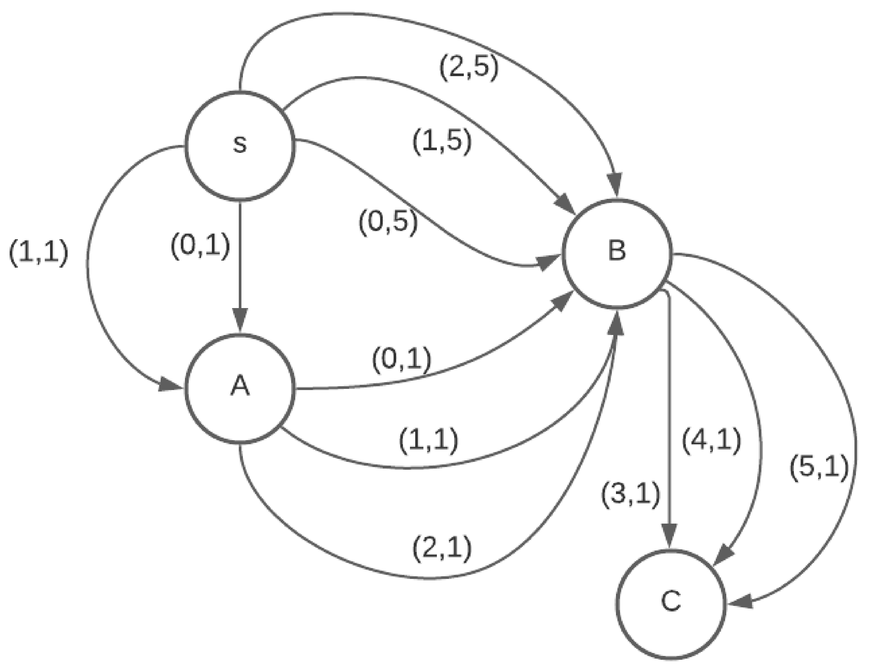
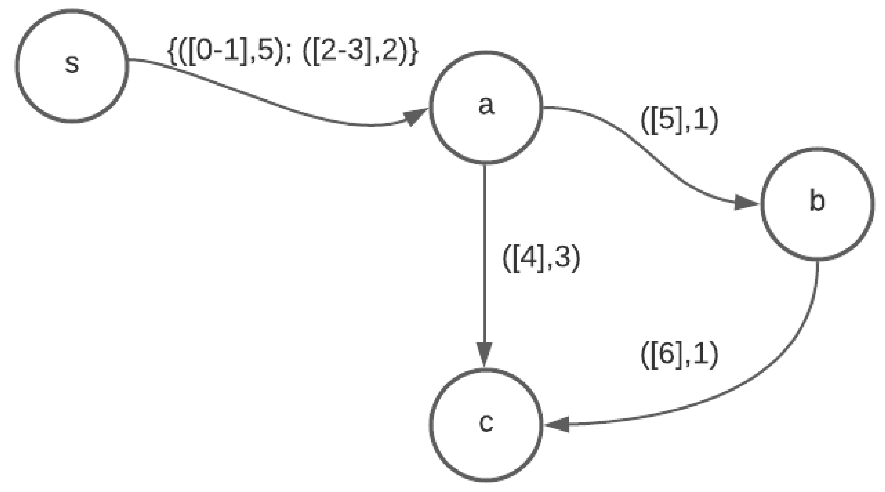
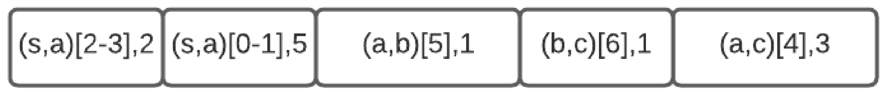
  • Temporal graph represented by data structure described in Section 5.4.1, item 1
  • Source vertex s
• OUTPUT:

  -

  Array $mwfWalks$ as described in Section 5.4.1, item 7

For simplicity, we assume that all the edge travel times are $>$0. Our algorithm for solving the $mwf$ problem (Algorithm 2) can easily be extended to the case when some travel times are $\ge$0. Later, we show how to carry out this extension. Algorithm 2 looks at all possible departure intervals in non-decreasing order of their arrival times when departing at the start of the interval ($intvl.strtTm+intvl.\mathsf{\lambda }$). In Step 8, it saves the arrival time of the latest interval being considered in the variable $curTm$. In the subsequent $while$ loop, it keeps fetching new intervals as long as they have the same arrival time as $curTm$, when departing at the start of the interval. For each fetched interval $newIntvl$, at the originating vertex u of $newIntvl$, it finds a walk class $prevW$ with latest arrival time of the start of the walk class $prevW.strtTm$ such that $prevW.strtTm\le newIntvl.st$. No other walk arriving at u needs to be considered for expansion on this interval due to Theorem 10. Using this previous walk at the originating vertex u, a new walk is created from u to v at the start of the $newIntvl$ using the function $createNewW$. This function creates a new walk from the previous walk departing at start of $newIntvl$ only if the second part of Theorem 12 is satisfied. The first part of Theorem 12 is already taken care of because the intervals are examined only in non-decreasing order of $intvl.st+intvl.\mathsf{\lambda }$.

Algorithm 2 Min-wait foremost walks algorithm

1: Create a new $newWClass\leftarrow (t_{start},\infty ,0,nbrs\_s\left[0\right])$ as an instance of $mwfWClass$. Values are assigned to fields $arrivTmStrt,arrivTmEnd,wtTm,lastExpAt$, respectively. Last field is an array of size out degree of vertex s. 2: Initialize mwfWalks[s]     ←   newWClass; initialize $listWClasses\left[s\right].pushback\left(newWClass\right)$; $\forall v\in V,v\ne s,mwfWalks\left[v\right]\leftarrow null$ 3: $nodesRchd\leftarrow 1$; $staticIntvls\leftarrow intvlList.size$; $indxStaticIntvls\leftarrow 0$ 4: $setupNewWClass(s,newWClass.arrivTmStrt)$ 5: $reachableNodes\leftarrow getReachableNodes(G,s)$ 6: $newIntvl\leftarrow removeMinIntvl\left(\right)$ 7: while ($(indxStaticIntvls<staticIntvls)$ or $!PQ.empty\left(\right)$) and $(nodesRchd<reachableNodes)$ do 8:     $curTm\leftarrow newIntvl.st+newIntvl.\mathsf{\lambda }$ 9:     $u=newIntvl.u$; $v=newIntvl.v$ 10:     $newVs\leftarrow 0$ 11:     while ($curTm==newIntvl.st+newIntvl.\mathsf{\lambda }$) do 12:         if $(newIntvl.v\ne s)$ then 13:            $prevWIndx\leftarrow getPrveW\left(newIntvl\right)$ 14:            if $prevWIndx\ne -1$ then 15:                $newW\leftarrow createNewW\left(listWClasses\right[u\left]\right[prevWIndx],newIntvl)$ 16:                if $newW$ then 17:                    $ins\leftarrow insNewW(newW,v)$   ▹ Inserts $newW$ in list of walks at v. If $newW$ is best $mwf$ walk it is recorded in $mwfWalks\left[v\right]$ 18:                    if $ins==NEW$ then 19:                        $newVs++$ 20:                    end if 21:                    if $ins\ne 0$ then 22:                        $setupNewWClass(v,newW.strtTm)$ 23:                    end if 24:                end if 25:            end if 26:         end if 27:         $newIntvl\leftarrow removeMinIntvl\left(\right)$ 28:     end while 29:     $nodesRchd+=newVs$ 30: end while

After the new walk is created on an edge $(u,v)$, it is appended to the list of walks at v. To qualify as a valid walk to be appended to the list of walks at v, it needs to be compared for dominance with only the last walk in the list at v due to Theorem 9. This walk is appended to the list at v only if it is not dominated. The insert function also checks if this is the first walk arriving at v. If so, it updates the $mwfWalks$ for vertex v and increments the count of $newVs$. If this is not the first walk to arrive at v, but if it is better w.r.t $mwf$ arrival than the best known walk at v, $mwfWalks$ is updated for vertex v. Note that the new walk cannot have an earlier arrival time than the best known walk at v as the intervals are examined in non-decreasing order of arrival times, but it may have a lesser wait time.

After a walk has been appended to the list of walks at v, the function $setupNewWClass$ examines all the neighbors of v. If the start time of the last arriving walk class is in the middle of an available departure interval, $intvl$ given, in the input graph G on an edge $(v,w)$, a new departure sub-interval of $intvl$, say $subIntvl$, is created. The start time of $subIntvl$ is the arrival time of the walk and travel time same as that of the $intvl$ ($intvl.\mathsf{\lambda }$). This way, every walk originates at the $start$ of an interval given in graph G or at start of a $subIntvl$ that is a sub-interval of one of the intervals given in the input graph G. This new $subIntvl$ is inserted into the priority queue $PQ$. In the $removeMinIntvl$ function, the interval with minimum arrival time (when departing at the start of the interval) from $intvlList$ and the top of $PQ$ is returned.

Theorem 16.

Algorithm 2 finds $mwf$ walks from s to all other vertices in an interval temporal graph when all edge travel times are $>$0.

Proof. 

The algorithm examines all the departure intervals in non-decreasing order of arrival time, when departing at the start of the interval. For every interval, $newIntvl$ in that order, it considers the best walk eligible for extension in this interval, as per Theorem 10, by obtaining the index for the previous walk ($prevWIndex$) in the list of walks at the departure vertex u, in Step 13. It extends the $prevWalk$ with departure in $newIntvl$ only if this extension is beneficial as per Theorem 12. Once the walk is extended, it updates the $lastExpAt$ for $prevWalk$ for the edge $(u,v)$, so that subsequent departure intervals on $(u,v)$ are used for expanding $prevWalk$ only if the resultant walks may be beneficial, as per Theorem 12.

The extended walk is appended to the list of walks at v only if it is not dominated as per the dominance criterion of Equation (1). In addition, $mwf$ walks at v are updated if the arriving walk is better than the previous $mwf$ walk, w.r.t $mwf$ arrival at v or if it is the first walk to arrive at v.

Finally, the arriving walk at v, $newW$, is examined w.r.t all outgoing edges $(v,w)$. If for a departure interval $I(s,e,\mathsf{\lambda })$ to any neighbor w we have $I_s<newW.strtTm\le I_e$, a new sub-interval, $subIntvl$, is created that has a start time of $newW.strtTm$ and inserted into $PQ$. When such a $subIntvl$ is the minimum interval among all the intervals from the input graph G and the $subIntvl$s created during the course of Algorithm 2, the $newW$ gets the opportunity to expand at the start time of $subIntvl$.

Therefore, this algorithm starts at the start vertex and generates walks at all feasible departure instances w.r.t $mwf$ walks criteria. Feasible departure intervals are examined in non-decreasing order of arrival times; therefore, every new walk generated has an arrival time ≥ arrival time of any previously generated walk. No feasible non-dominated walk is missed due to Theorems 8–13.

Every non-dominated walk generated is preserved and expanded as per Theorems 11–13. When a walk terminating at a vertex v is discovered that is the best among the walks arriving at v w.r.t $mwf$ arrival, it is recorded as the $mwf$ walk at v. The algorithm terminates only when one of the following is true

• All intervals including the $sub-intervals$ created during the course of Algorithm 2 have been examined.
• $mwf$ walks to all reachable vertices have been found and the arrival time when departing at the start of next interval being examined is bigger than the max arrival time of the $mwf$ walks found. Therefore, examining any more intervals cannot give a better $mwf$ walk.

Therefore, when the algorithm terminates, $mwf$ walks to all reachable vertices have been found. □

For handling the case when some travel times are 0, in the while loop of line 11, we need to first obtain all the edges with 0 travel times arriving at $currTm$ and form their transitive closure. Then, we can process every edge arriving at the same $currTm$ over this transitive closure.

Theorem 17.

When time is an integer, Algorithm 2 has pesudopolynomial complexity.

Proof. 

Let T be the maximum possible arrival time at any vertex. Since $curTm$ is an integer that increases in each iteration of the outer while loop, this outer loop is iterated $O\left(T\right)$ times. For each value of $curTm$, the while loop of line 11 is iterated $O\left(M_{itg}T\right)$ times, where $M_{itg}$ is number of edges in the input interval temporal graph, as the number of walks that can arrive at a vertex v at time $curTm$ is $O\left(indegree\right(v)\ast T)$. The components of the time required for each iteration of the while loop of line 11 are

• $log\left(walks\right(v\left)\right)$ in step 13 to find the previous walk that can be extended at the current departure instance($t_{arr}$). $walks\left(v\right)$, which is the number of walks at v at time $t_{arr}$, can be at most $t_{arr}$ as each preserved walk at a given vertex v has a unique arrival time. Therefore, time taken by this step is $log\left(t_{arr}\right)$ or at most $log\left(T\right)$.
• Constant time for creating a new walk $newW$ in step 15.
• Constant time for inserting $newW$, in the list of walks l at v in step 17. l at every vertex v maintains a list of walks that has arrived at v in non-decreasing order of their arrival times. $newW$ only needs to be compared with the last walk in l.
• At most $dlog\left(\delta \right)$ in step 22, d is the out-degree of the vertex v at which $newW$ terminates and $\delta$ is the number of departure intervals on an outgoing edge $(v,w)$ that has maximum departure intervals among all the outgoing edges from v. Each of the departure intervals on outgoing edges from v may need to be added to $PQ$.
  Size of $PQ$ can be, at most, the maximum number of departure instances in the graph G, which is $M_{itg}T$. Therefore, the maximum time taken in this step is $dlog\left(\delta \right)log\left(M_{itg}T\right)$.
• Finally, in step 27, departure instance with minimum arrival time is retrieved. Maximum size of $PQ$ can be $M_{itg}T$. Therefore, maximum time taken by this step is $log\left(M_{itg}T\right)$

Therefore, the complexity of the algorithm is $O\left(T\right(M_{itg}T(log\left(T\right)+dlog\left(\delta \right)$$log\left(M_{itg}T\right)+log\left(M_{itg}T\right)\left)\right))$, which is $O(M_{itg}{T}^{2}log\left(T\right))$. Hence, the time complexity of Algorithm 2 is pseudopolynomial. □

6. Linear Combination of Optimization Criteria

Bentert et al. [10] present a polynomial time algorithm that optimizes any linear combination of the eight optimization criteria $foremost$, $reverse\_foremost$, $fastest$, $shortest$, $min\_hop$, $cheapest$, $most\_likely$, and $min\_wait$ in a contact-sequence temporal graph. In this section, we show that, when time is discrete, we can use the algorithm of Bentert et al. [10] to solve the $mhf$, $mwf$ and $mcf$ problems in polynomial time for contact-sequence graphs. This algorithm may also be used to find $mhf$, $mwf$, and $mcf$ paths in interval temporal graphs by first transforming the interval-temporal graph into an equivalent contact sequence graph as described in Section 1. Since this transformation may increase the number of edges by an exponential amount, this approach does npt result in a polynomial time algorithm for interval-temporal graphs. However, it does result in a pseudopolynomial time algorithm as shown in Theorem 17.

To solve $mhf$, for example, for contact-sequence graphs, we perform the following:

• Set the coefficient for every criterion other than $min\_hop$ and $foremost$ to 0.
• The coefficient for the foremost criterion may be set to any integer that is greater than or equal to the number of vertices, n, in the contact-sequence graph.
• Set the coefficient for the min-hop criterion to 1.

With these settings, Bentert et al. [10] will find walks that minimize $h(s,v)=c_f\ast t_a\left(v\right)+hops\left(v\right)$, where $c_f$ is the coefficient for the foremost criterion, $t_a\left(v\right)$ is the time at which the walk from s arrives at v, and $hops\left(v\right)$ is the number of hops in the walk. Since a min-hop walk is necessarily a min-hop path, it has no more than $n-1$ hops. If we examine the digits of $mhf(s,v)$, which is a non-negative integer, using the radix $c_f$, the least significant digit is the number of hops and the remaining digits give $t_a$. Hence, $mhf(s,v)$ is minimized by min-hop foremost paths to v and not by any other path or walk.

The strategy for $mwf$ and $mcf$ is similar. In the case of $mwf$, the function to optimize is $mwf(s,v)=c_f\ast t_a\left(v\right)+wait(s,v)$ and for $wcf$, the optimization function is $wcf(s,v)=c_f\ast t_a\left(v\right)+cost(s,v)$, where $wait(s,v)$ is the total wait time on the walk from s to v and $cost(s,v)$ is its cost. For $mwf(s,v)$, $c_f$ must be larger than the maximum total wait time on an optimal foremost walk from s (a simple bound is the maximum arrival time of a foremost path to reachable vertices), and for $mcf(s,v)$, $c_f$ must be larger than the maximum cost of an optimal foremost path (a simple bound to use is the sum of the maximum cost of each edge). For simplicity, we use $c_f=2^{32}$ in our experiments, as this is large enough for our data sets.

It is easy to see how the above modeling strategy may be used to find, say, min-cost foremost paths with the fewest number of hops.

7. Experimental Results

In this section, we compare the performance of our $mhf$ path and $mwf$ walk algorithms to the algorithm of Bentert et al. [10]. Since the latter algorithm works only on contact-sequence graphs, we first transform our interval-temporal graphs into equivalent contact-sequence graphs (as noted in Section 1, this can be performed when time is discrete) and then we use the strategy discussed in Section 6 to formulate an appropriate optimization function for the algorithm of Bentert et al. [10]. Since the optimization function constructed in Section 6 has values larger than what can be handled by the datatype int, we modified the code of Bentert et al. [10] using the datatype long for relevant variables.

Our experimental platform was an $IntelCore,i9-7900XCPU@3.30GHz$ processor with 64 GB RAM. The C++ codes for finding the optimal linear combination of multiple optimization criteria for contact-sequence temporal graph algorithms was obtained from the authors of [10]. All other algorithms were coded by us in C++. The codes were compiled using the $g++ver.7.5.0$ compiler with option O2. For test data, we used the datasets used in [8,10], for the contact-sequence graphs. We transformed these contact-sequence graphs to interval-temporal graphs to run on our algorithms. We also generated some synthetic datasets as interval-temporal graphs that we transformed to contact-sequence models so the programs of Bentert et al. [10] could be run on them.

7.1. Datasets

We used 13 of the 14 real-world contact-sequence graphs that were used in [8,10,12,13]. The 14th dataset, dblp, was not used as it had a few negative timestamps. The statistics for the remaining 13 real-world datasets are given in

Table 1. Koblenz collection graph statistics.

Dataset	$\left|\mathit{V}\right|$	$|{\mathit{E}}_{\mathit{s}}|$	$\mathit{cs}-\mathit{edges}$	Activity
epin	131.8 K	840.8 K	841.3 K	1
elec	7119 K	103.6 K	103.6 K	1
fb	63.7 K	817 K	817 K	1
flickr	2302.9 K	33,140 K	33,140 K	1
growth	1870.7 K	39,953 K	39,953 K	1
youtube	3223 K	9375 K	9375 K	1
digg	30.3 K	85.2 K	87.6 K	1.02
slash	51 K	130.3 K	140.7 K	1.07
conflict	118 K	2027.8 K	2917.7 K	1.43
arxiv	28 K	3148 K	4596 K	1.45
wiki-en-edit	42,640 K	255,709 K	572,591 K	2.23
enron	87,274	320.1 K	1148 K	3.58
delicious	4512 K	81,988 K	301,186 K	3.67

. In this table, $\left|V\right|$ is the number of vertices, $|E_s|$ is the number of edges in the underlying static graph and $cs-edges$ is the number of edges in the contact-sequence temporal graph. The ratio $(cs-edges)$/$|E_s|$ is the temporal activity of the graph. Note that the number of edges in the interval-temporal graph is also $|E_s|$. The datasets have a wide range of sizes in terms of the number of vertices and edges. Consistent with [8,10,12,13], the travel time, $\mathsf{\lambda }$, on all edges was set to 1. The temporal activity on these datasets is low, ranging from 1 to $3.67$.

In [13], we generated five synthetic datasets with higher activity and variable $\mathsf{\lambda }$s by starting with the social network graphs of youtube, flickr, livejournal shared by the authors of [17] at http://socialnetworks.mpi-sws.org/data-imc2007.html (accessed on 16 August 2022). These graphs represent user-to-user interactions.

Table 2. Synthetic graphs statistics.

Graphs with ${\mathit{\mu }}_{\mathit{I}}=4,{\mathit{\mu }}_{\mathit{D}}=5,{\mathit{\mu }}_{\mathit{T}}=3$
Dataset	$\left|V\right|$	$|E_s|$	cs-edges	Edge Activity
youtube	1157.8 K	4945 K	105,039 K	21.2
flickr	1861 K	22,613.9 K	480,172 K	21.24
livejournal	5284 K	77,402.6 K	1,643,438 K	21.3
Graphs with ${\mu }_I=4,{\mu }_D=8,{\mu }_T=3$
youtube	1157.8 K	4945 K	159,103.7 K	32.1
flickr	1861 K	22,613.9 K	727,405.9 K	32.1

shows the statistics for the five synthetic temporal graphs generated by us.

Table 3. Reading times and sizes.

Koblenz Collection
Dataset	Reading Time (in s)		Sizes in MBs
	[10]	Ours	[10] Graph	Ours
epin	0.46	0.34	31.1	19.3
elec	0.13	0.07	4.5	3.3
fb	0.58	0.34	32.9	21.5
flickr	19.3	14.2	1492.3	911
growth	27	19.9	2188.3	1485.4
youtube	6.1	4.2	456.1	300.8
digg	0.11	0.06	3.6	2.5
slash	0.14	0.07	7	5
conflict	1.44	0.82	98.8	43.2
arxiv	2.5	1.4	193	104
wiki-en-edit	–	227	out-of-mem	20,115
enron	0.74	0.36	55.9	29.3
delicious	209	78	16,249	7552
Synthetic Datasets with ${\mu }_I=4,{\mu }_D=5,{\mu }_T=3$
youtube	67	4	4400	272.2
flickr	–	17.8787	out-of-mem	1248
livejournal	–	56.1638	out-of-mem	4411
Synthetic Datasets with ${\mu }_I=4,{\mu }_D=8,{\mu }_T=3$
youtube	102	3	6775	272
flickr	–	18	out-of-mem	1249

gives the time (in seconds) required to read each dataset from the disk as well as the disk memory required by each dataset. The columns labeled [10] are for the case when the dataset is stored in the input format used by the algorithm of Bentert et al. [10] and those labeled Ours are for the input format required by our algorithm. As can be seen, the disk reading time and disk space required by the interval-temporal graph representation are less than that required by the Bentert et al. [10]. Further, this difference increases as the temporal activity increases. In fact, for four of the instances, input creation code of [10] failed to create the required input format for lack of sufficient memory (out-of-mem).

As an example, for the large synthetic $youtube$ graph with $({\mu }_I=4,{\mu }_D=8,{\mu }_T=3)$ which has an activity factor of $32.1$, the reading time of the interval-temporal graph is $3.53$ s while the program by Bentert et al. [10] takes about $102.5$ s to read the corresponding graph in Bentert’s transformed format. The size of the interval temporal graph for the same dataset on disk is $272.3$ MB as compared to $6.7$ GB for the Bentert’s transformed graph from the corresponding contact-sequence graph.

7.2. Run Times

As in [8,10,12,13], we assume that the the graph is resident in memory (i.e., the read time from disk is not accounted for). This is a valid assumption in applications where the graph is input once and queried many times. To use the algorithm of Bentert et al. [10], we use the following steps:

• Transform the interval temporal graph to an equivalent contact sequence graph ($csg$) as described in Section 1.
• Use Bentert’s graph transformation program [10] to convert the $csg$ to the input format used by Bentert’s linear combination algorithm.
• Run Bentert’s linear combination program on the transformed graph from Step 2 using the coefficients given in Section 6.

The step 2 transformation was unsuccessful on the Koblenz dataset $wiki-en-edit$ as well as on all our synthetic datasets other than $youtube$ graph with $({\mu }_I=4,{\mu }_D=5,8,$${\mu }_T=3$), as indicated in Table 3. The failure of this step resulted from the unavailability of sufficient memory to run the step 2 transformation code of [10] on these instances. We measured the average of the runtimes for 100 randomly selected source vertices for each dataset except the $delicious$ from the Koblenz collection and the synthetic datasets, where we used only five randomly selected source vertices. This reduction in the number of source vertices was necessary because of the excessive runtime taken by the algorithm of [10] on these datasets. The average run-times (in seconds) for the Koblenz and synthetic datasets are given in

Table 4. Runtimes in seconds.

Koblenz Datasets
Dataset	$\mathit{mhf}$			mwf
	$\mathit{mhf}$-[10]	$\mathit{mhf}$-Ours	$\mathit{mhf}$-[10]/Ours	$\mathit{mwf}$-[10]	$\mathit{mwf}$-Ours	$\mathit{mwf}$-[10]/Ours
epin	0.04	6.6 × 10${}^{-3}$	6.106	0.04	0.02	2
elec	1.3 × 10${}^{-2}$	3.6 × 10${}^{-4}$	36	0.01	0.003	3.33
fb	1.8 × 10${}^{-2}$	1.1 × 10${}^{-3}$	15.9	0.017	0.03	0.56
flickr	5.57	0.45	12.34	5.65	1.37	4.12
growth	9.56	1.67	5.72	9.95	4.2	2.36
youtube	0.32	1.2 × 10${}^{-2}$	25.8	0.33	0.18	1.83
digg	2.1 × 10${}^{-3}$	9.1 × 10${}^{-5}$	23.66	0.002	0.002	1
slash	0.01	1.3 × 10${}^{-3}$	11.17	0.01	0.005	2
conflict	9 × 10${}^{-5}$	3 × 10${}^{-5}$	3	0.0009	0.02	0.045
arxiv	5 × 10${}^{-2}$	9.3 × 10${}^{-3}$	6.25	0.06	0.15	0.4
enron	0.18	2.8 × 10${}^{-3}$	64.11	0.7	0.03	23.3
delicious	222	1.07	207.5	763	41	18.6
Synthetic datasets ${\mu }_I=4,{\mu }_D=5,{\mu }_T=3$
youtube	120.8	0.17	679.5	186.8	71.3	2.6
Synthetic runtimes ${\mu }_I=4,{\mu }_D=8,{\mu }_T=3$
youtube	132.7	0.29	451.3	275	95.5	2.8

. This time does not include the time required by steps 1 and 2. The speedups (time taken by the algorithm of [10]/time taken by our algorithm) are also shown visually in Figure 13, Figure 14, Figure 15 and Figure 16.

The speedups obtained by our $mhf$ algorithm over [10] range from 3 to $207.5$ for the Koblenz datasets and from $451.3$ to $679.56$ for the synthetic datasets. Our $mhf$ algorithm outperforms that of [10] on all datasets. The speedups obtained by our $mwf$ algorithm over [10] range from a low of 0.045 to a high of $23.3$. The algorithm of [10] outperforms our $mwf$ algorithm when the graph has very low connectivity. Their algorithm is able to quickly discover that no more vertices are reachable from the source vertex and, so, terminates sooner than our $mwf$ algorithm. However, when there are many reachable vertices, our algorithm outperforms that of Bentert et al. [10]. We also note that our algorithm works on interval-temporal graphs where time intervals may be continuous or have large durations, while the algorithm of Bentert et al. [10] is only for contact-sequence graphs, which are a subset of interval temporal graphs. As noted earlier, the algorithm of [10] could not be run on some datasets because of the failure of step 2 as it ran out of memory. On the four datasets where the algorithm of [10] could not be run, the average runtime of our $mhf$ algorithm was 1, 1.1, 1.3, and 22.2 s, respectively; the runtime for our $mwf$ algorithm was $39.1$, $368.4$, 449 and $1317.6$ s, respectively.

8. Conclusions

We have shown that finding $mwf$ paths and walks as well as $mcf$ paths in interval-temporal graphs is NP-hard. For the $mhf$ single-source all-destinations problem, a polynomial time algorithm was developed and for the $mwf$ single-source all-destinations problem, a pseudopolynomial time algorithm was developed. We show also that the $mhf$ and $mwf$ problems for interval graphs can be solved using the linear combination algorithm of Bentert et al. [10] for those interval graphs that can be modeled as contact-sequence graphs. While the algorithm of [10] is polynomial in the size of the contact-sequence graph, the modeling of an interval-temporal graph by a contact-sequence graph, when possible, may increase the graph size by an exponential amount and, so, this approach does not result in a polynomial time algorithm for interval-temporal graphs. In fact, even though all of our datasets could be modeled as contact-sequence graphs, we were unable to use the algorithm of [10] on one of our Koblenz datasets and three of our synthetic datasets as the code of [10] that transform the contact-sequence graph into the required input format failed due to insufficient memory. Our $mhf$ paths algorithm outperformed the linear combination algorithm of [10] on all datasets on which the algorithm of [10] could be run. A speedup of up to $69.9$ was obtained on the Koblenz datasets and up to 679 on synthetic datasets. For the $mwf$ single-source all-destinations problem, which is NP-hard, the linear combination algorithm of [10] outperformed our algorithm on three of the Koblenz data sets and tied on a fourth. On all remaining datasets, our algorithm outperformed that of [10]. The datasets on which the algorithm of [10] did well had the property that few vertices were reachable from the source vertex. This enabled the algorithm of [10] to terminate early. In these cases, the speedup obtained by our algorithm ranged from 0.045 to 0.56. On the remaining Koblenz datasets, our $mwf$ algorithm obtained a speedup of up to $23.3$. For both the synthetic datasets where it was possible to run the algorithm of [10], our algorithm was faster and delivered a speedup of up to 2.8. On the four datasets that the transformation to the input format required by the algorithm of [10] failed due to lack of memory, our $mhf$ algorithm ran in 1, 1.1, 1.3, and 22.2 s, respectively and the runtime for our $mwf$ algorithm was $39.1$, $368.4$, 449 and $1317.6$ s, respectively.