Long-Term EEG Component Analysis Method Based on Lasso Regression

Abstract

At present, there are very few analysis methods for long-term electroencephalogram (EEG) components. Temporal information is always ignored by most of the existing techniques in cognitive studies. Therefore, a new analysis method based on time-varying characteristics was proposed. First of all, a regression model based on Lasso was proposed to reveal the difference between acoustics and physiology. Then, Permutation Tests and Gaussian fitting were applied to find the highest correlation. A cognitive experiment based on 93 emotional sounds was designed, and the EEG data of 10 volunteers were collected to verify the model. The 48-dimensional acoustic features and 428 EEG components were extracted and analyzed together. Through this method, the relationship between the EEG components and the acoustic features could be measured. Moreover, according to the temporal relations, an optimal offset of acoustic features was found, which could obtain better alignment with EEG features. After the regression analysis, the significant EEG components were found, which were in good agreement with cognitive laws. This provides a new idea for long-term EEG components, which could be applied in other correlative subjects.

1. Introduction

Emotions play an essential role in human intelligence activities. The research of affective computing has wide application prospects. A deep understanding of emotions could help people shake off depression and improve work efficiency. Current research on affective computing mainly focuses on voice, images, and multi-modal physiological information [1]. The research on visual information inducing emotion started earlier, and the results are more comprehensive and richer, including emotional pictures, facial expressions, videos, and games [2]. Music is an art that expresses and inspires emotions by the difference in melody, the speed of the rhythm, the height of the volume, the change of the harmony, and the different kinds of timbre. It conveys emotional information more directly than language [3]. Therefore, music is an ideal breakthrough for studying human emotional activities [4].

At present, the understanding of emotion includes two levels: one is emotional expression, and the other is emotional experience. Emotional expression is mainly the emotion expressed in music, pictures, and other works, while emotional experience includes cognitive factors [5]. Research on the cognitive brain mechanism of music emotions has mainly been completed by electroencephalogram (EEG) and functional magnetic resonance imaging (fMRI) [6]. Specific brain activities can be observed by fMRI in the form of pictures. However, due to a low temporal resolution, it cannot accurately analyze the dynamic activities of the brain. EEG signals can be used to explore cognitive principles and to perceive emotional states [7]. Compared with audio and visual images, EEG signals not only contain perceptual information, but also cognitive information, which can better express an emotional experience. Compared with EMG, EEG is the brain’s natural reflection of information, which can accurately analyze the dynamic activities of the brain. Therefore, EEG signals are selected to study long-term emotions. However, the research on EEG emotion is still in the primary stage, and the research objects are simple notes. The lack of intrinsic features and calculation models of long-term EEG greatly limits the development of affective computing. Therefore, a long-term EEG signal analysis method is necessary, which could more scientifically and accurately reflect emotional changes, and deeply explore the cognitive principle of emotion and brain.

In this article, a long-term EEG component analysis method based on Lasso regression is proposed, which could analyze long-term and continuous EEG signals, and find emotion-related components.

1.1. Related Works of Emotional EEG Analysis

Temporal signals carry emotional information. The research of dynamic emotion recognition attempts to identify an emotional state based on information before that moment, which is also the process of people’s perception of emotions. Madsen et al. [8] found that the temporal structure of music is essential for musical emotion cognition. Based on the kernel Generalized Linear Model (kGLM), they obtained a lower classification error in both continuous emotions (valence, arousal) and discrete emotion recognition. Saari et al. [9] obtained a better emotion prediction effect by extracting long-term semantic features. They built large-scale predictive models for moods in music based on the semantic layer projection (SLP) technique, and obtained prediction rates from moderate (R2 = 0.248 for happy) to considerably high (R2 = 0.710 for arousal). Han’s research team found a higher emotion recognition rate by merging frame-based timing information and long-term global features [10]. They proposed a global-control Elman (GC-Elman) network to combine utterance-based features and segment-based features together and obtained a recognition rate for anger, happiness, sadness, and surprise of 66.0%. These studies have proved that there are emotion-related cues in time-series information, which is of great help to emotion prediction.

Then question, then, is how to describe emotional changes in long-term brain activity. The EEG is a complex non-stationary random signal which is easily disturbed by the external environment and subject movement [11]. At present, the most commonly used methods of EEG analysis are event-related processing methods such as event-related potentials (ERP), event-related synchronization (ERS), and event-related desynchronization (ERD) [12]. The principle is that the specific stimulus could cause regular potential changes in the brain. Therefore, neural activity in the cognitive process could be measured through the electrophysiological changes of the brain [13]. Poikonen et al. [14] successfully extracted the N1 and P2 components caused by music through the ERP technique. The potential changes are similar to the same type of stimulus, while the noise in response is random. Therefore, the ERP component could be obtained, and the random noise balanced out, by large amounts of superposition and averages of EEG, as shown in Figure 1. The horizontal axis represents time and the vertical axis represents voltage amplitude. Furthermore, by analyzing the contribution of the ERP component, the EEG component that has the largest contribution could be found. The numbers (1, 3, 4, 7, 8, 11, and 13) on the topographic maps are the index of the independent components of EEG signals, which were obtained by Independent Component Analysis.

At present, most EEG signal processing methods are aimed at short-term brain activities, and there are few analysis methods for long-term EEG response. Among many analysis methods, the power spectral density analysis and Auto-Regressive (AR) model estimation are frequently used. Power Spectral Density (PSD) represents a power change with a frequency, that is, the distribution of signal power in the frequency domain. Generally, the nonparametric estimation, based on Fourier transform, is used for PSD calculation. The power spectrum estimation method proposed by Welch [15] is widely used. Li et al. combined PSD and brain topographic maps for visualizing energy changes of different frequency bands of long-term EEG [16]. The band energies of EEG signals were calculated with sliding windows and plotted on brain topographic maps in chronological order. With music playing, the change process of brain activity could be dynamically displayed and measured. The Auto-Regressive (AR) Model [17] is a linear regression model that combines previous information to describe a random variable at a specific time. It is essentially a linear prediction. Zhang et al. [18] used the AR model and empirical mode decomposition (EMD) to extract EEG features for emotion recognition induced by music videos. The average recognition rate of four kinds of emotions was 86.28%. In addition, Li et al. [19] extended the brain functional network method to analyze dynamic EEG changes during music appreciation. The dynamic brain functional network for different frequency bands of EEG signals was constructed by mutual information, observed over time, and used in emotion recognition. Based on the SVM classifier, the recognition rate of the four categories of emotion music classification —happy, distressed, bored, and calm—is 53.3%.

In addition to the above processing methods, various intelligent processing methods have vigorously promoted emotional EEG signal analysis. In 2007, Murugappan et al. extracted two chaotic features (Fuzzy C-Means, Fuzzy K-Means) of EEG signals and applied them to emotion classification [20]. In 2010, Lin from the National Taiwan University used a differential asymmetry of electrodes to classify five types of emotions induced by music, and achieved a recognition rate of 82% [21]. In 2012, the Greek scholar Panagiotis proposed Higher Order Crossings features to classify six types of emotions (happiness, surprise, anger, fear, disgust, and sadness) and obtained a recognition rate of 83% [22]. In 2017, Samarth et al. applied the deep neural network (DNN) and convolutional neural network (CNN) to recognize emotions. The recognition rate of two types of emotions reached 73.36%, based on multimodal physiological signals. The recognition rate of three kinds of emotions was 57.58% [23].

It is not difficult to see that most existing analysis methods are based on statistical analysis and machine learning techniques. There are many deficiencies in the research of long-term brain cognitive mechanisms and emotion recognition. The main reasons are as follows:

(1)

There is no long-term analysis method of EEG components, or quantitative calculation method for EEG features;

(2)

In most of the existing methods, temporal information is ignored, and the characteristics of temporal variation of emotions are not considered.

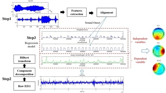
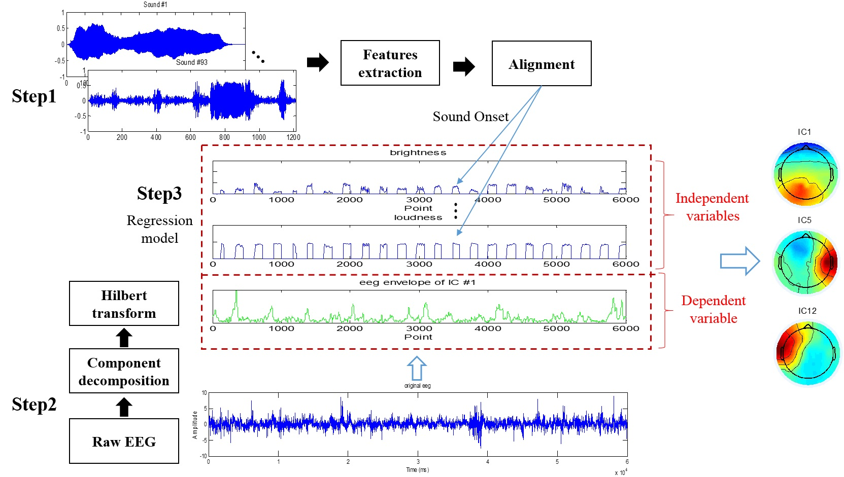
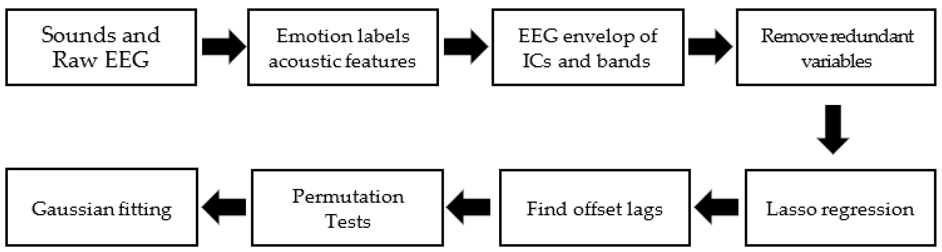
1.2. The Proposed Method and Article Structure

Due to the lack of component analysis and quantitative calculation of long-term EEG signals, a new method of time-varying feature analysis based on Lasso regression analysis is proposed in this article.

First of all, a cognitive experiment through continuous sounds was designed, and the EEG signals were recorded. Secondly, the emotion-related acoustic features of the sounds were extracted and calculated. Moreover, the EEG components were separated by the Independent Component Analysis (ICA) analysis method, and a regression model between the EEG components and acoustic features was established to reveal long-term correlations. Finally, the most relevant emotion-related EEG components were found by the random arrangement test and Gaussian fitting. Compared with short-term EEG emotion prediction, the long-term analysis method proposed in this article has the advantages of a longer analysis time and more accurate prediction results. The probability of finding abnormal brain waves is higher, and the chance of a missed diagnosis is reduced.

The main content is as follows: Section 2 briefly introduces the basic principles and methods of the long-term analysis method of EEG components. Section 3 explains the cognitive experiment and gives the experimental results. In Section 4, the advantages of the proposed method are discussed, and possible further improvements are given.

2. Methods

The process of the method proposed in this article is shown in Figure 2. It mainly included the following four steps: (1) extracting the acoustic features of the audio and finding the emotion-related acoustic features based on correlation analysis; (2) ICA decomposition and features extraction of EEG signals; (3) time-varying regression analysis between acoustic features and EEG components; and (4) finally, looking for the most relevant emotion-related EEG components by permutation tests and Gaussian fitting.

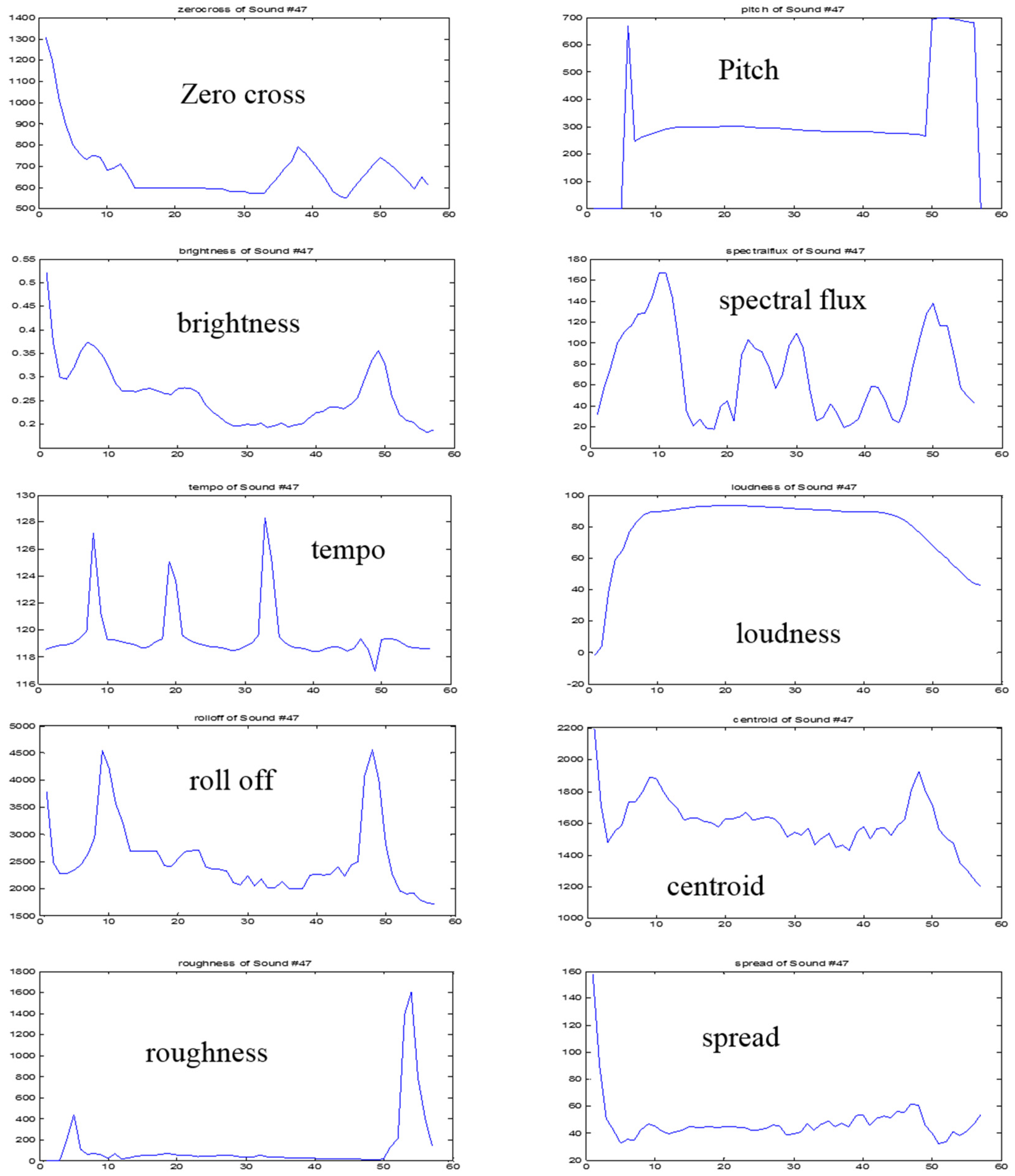
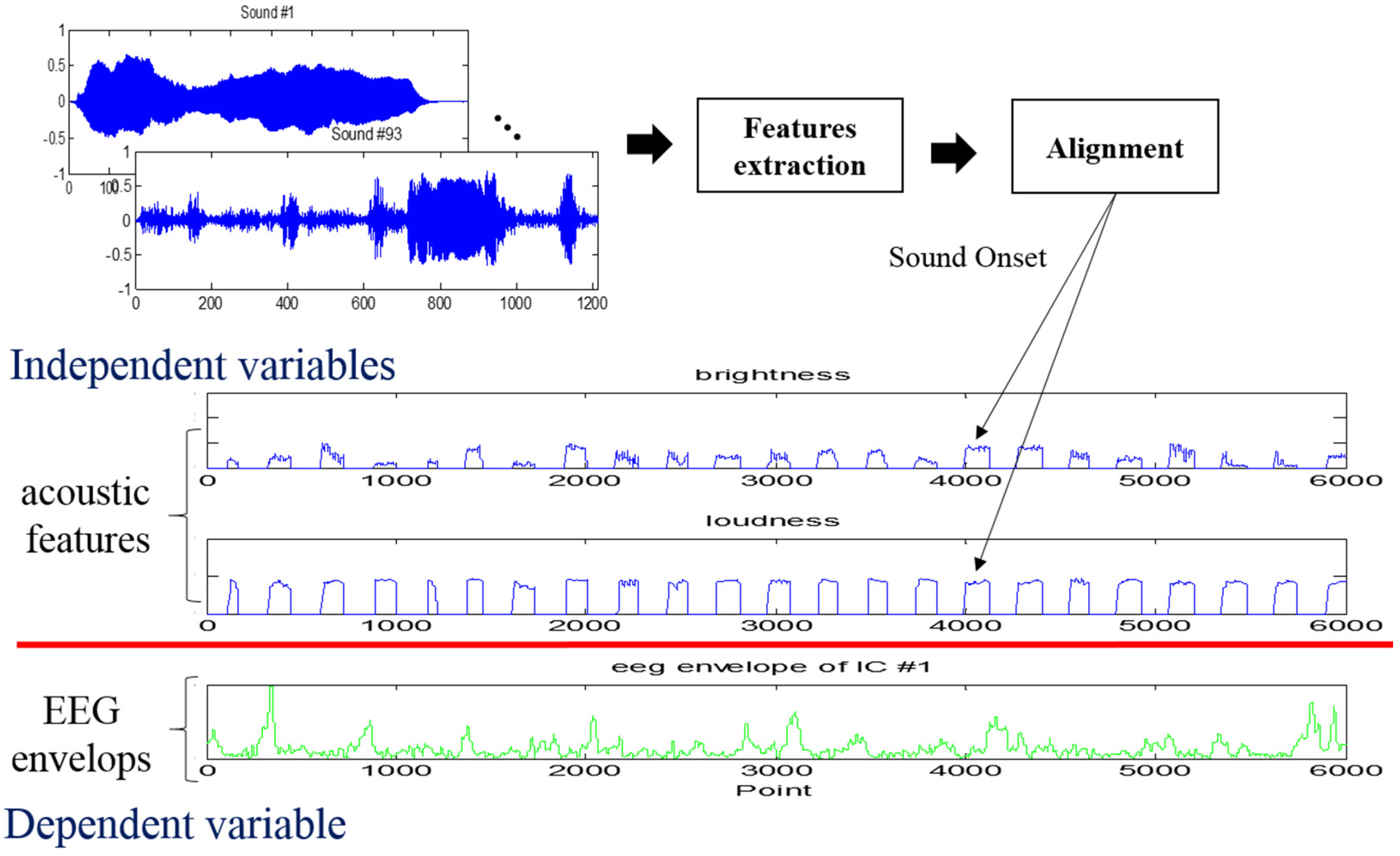
2.1. Acoustic Feature Extraction

In the current auditory recognition methods, acoustic features are extracted in the form of frames. The extraction process is as follows: (1) divide the audio signal into frames; (2) extract features for each frame; (3) calculate the first-order difference of the frame features; and (4) finally use the frame feature and the mean-variance of the first-order difference as the feature of the entire audio.

There are 48 dimensions in the feature set, including low-level descriptors: the loudness, root-mean-square signal frame energy, intensity, loudness, 12 MFCC, pitch (F0), its envelope, F0 envelope, 8 line spectral frequencies, and zero-crossing rate; and the statistical values of these features are: the maximum, minimum, range, arithmetic mean, two linear regression coefficients, linear and quadratic error, standard deviation, skewness, kurtosis, quartile 1–3 and 3 inter-quartile ranges, and delta regression coefficients. These are taken from the OpenSMILE configuration file for the IS09 emotion challenge, which were also used in [24] and [25]. In the process of the feature extraction of the sound signal, the frame length is set to 50 ms, and the frame shift is 10 ms, which is easy to align with the envelope of the EEG.

The correlation analysis based on the similarity matrix is used for feature dimension reduction. The construction method is as follows:

First of all, set the music signal as $A_i, 1\le i\le N$ (N is the number of samples) and acoustic features as $F_i, 1\le i\le M$ (M is the feature dimension). The feature set (F) includes low-level features such as pitch, zero-crossing rate, and loudness, as well as high-level semantic features, such as brightness, and roughness. The behavior ratings of emotion labels (valence and arousal) are L. As discussed above, the human brain’s response to music is based not only on the audio information at the current moment, but also on the time before the current moment. To preserve the time information, the audio feature $F_i$ is windowed and divided into frames.

Secondly, construct a feature similarity matrix (FDM) for each feature and a label similarity matrix (LDM) for the valence and arousal ratings. The feature similarity matrix (FDM) is built as follows:

$$FD{M}_{pg}=dist\left(F^p,F^q\right), 1\le p,q\le N$$

(1)

where $F^p$ and $F^q$ represent the feature vector of the p-th sample and the q-th sample, and dist(X,Y) represents the cosine similarity between X and Y.

$$dist\left(X,Y\right)=\frac{\overrightarrow{x}·\overrightarrow{y}}{\Vert x\Vert ·\Vert y\Vert }$$

(2)

The distance function could be Euclidean distance, Mahalanobis distance, and Cosine similarity. To test the performance of distance function, 259 initial samples were divided into two categories: living sound and nonliving sound, which have been proved to be quite different [26]. The similarity matrices of the same feature were calculated, respectively, by using Euclidean distance, Mahalanobis distance, and cosine similarity, shown in Figure 3. There were two groups: the first 125 samples were living sounds and the last 134 samples were nonliving sounds. The difference between the two groups was used as the selection criteria. The distances with a large difference between groups, and a small difference within groups were used. Here, cosine similarity was selected, which could better describe the difference of specific feature vectors.

Thirdly, calculate the similarity between FDM and LDM matrices, as the similarity score S₁, the calculation formula is as follows:

$$S_1=\frac{FDM\cdot LDM}{\Vert FDM\Vert \cdot \Vert LDM\Vert }=\frac{{\displaystyle \sum _{i=1}^n}FD{M}_i\times LD{M}_i}{\sqrt{{\displaystyle \sum _{i=1}^n}{(FD{M}_i)}^2}\times \sqrt{{\displaystyle \sum _{i=1}^n}{(LD{M}_i)}^2}}$$

(3)

Finally, the row values of $FD{M}_i$ represent the distances between $A_i$ and $A_j$, 1 ≤ j ≠ i ≤ N in a specific feature. It could measure the feature similarity between samples. Therefore, set S₂ is the feature similarity between samples, which could be calculated by the sum of the row value of FDM. The final similarity score S for a specific feature is given by:

S = S₁ + S₂

(4)

By sorting S, the most relevant features ${\widehat{F}}_i, 1\le i\le K$ of emotions could be found.

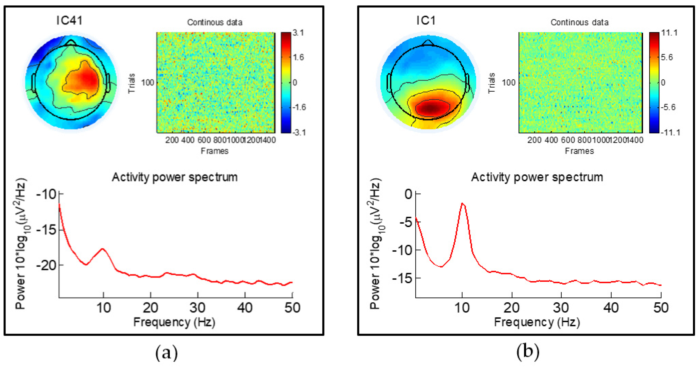
2.2. EEG Component Decomposition and Feature Extraction

It is widely known that the EEG component is very weak, and the noise is very strong. As the EEG signal is only about 50 mV, preprocessing is necessary. The process of EEG signal processing is shown in Figure 4.

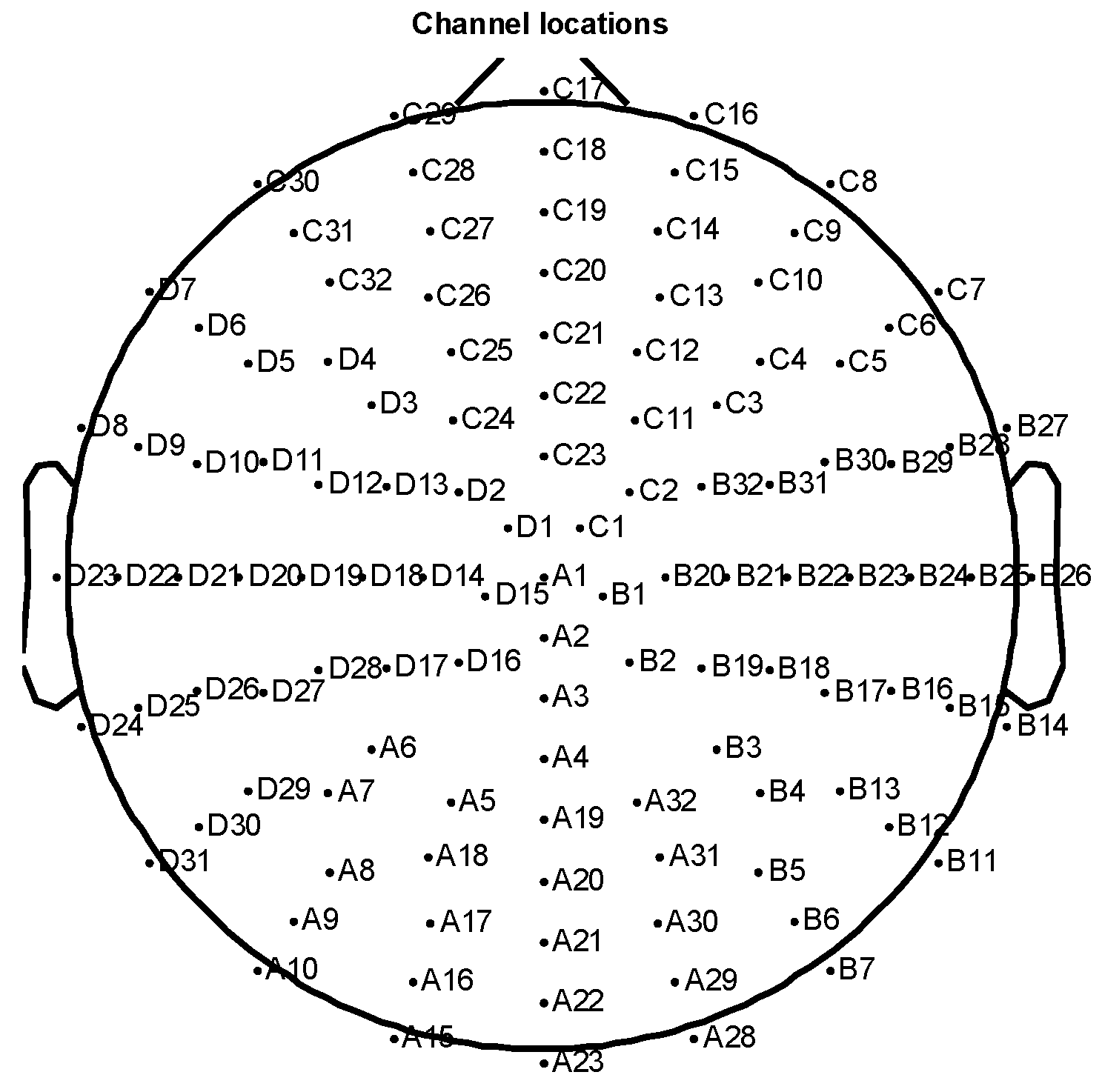
2.2.1. EEG Preprocessing

To reduce interference, the left mastoid is selected as the reference electrode. In contrast, the average reference is usually used to amplify the fluctuation of amplitude in data analysis. That is, the EEG data is obtained by subtracting the average value of all channels.

Then, because the effective frequency of the EEG signal is mainly concentrated below 50 Hz, a band-pass filter from 0.5 to 50 Hz is applied to the EEG signal. The finite impulse response (FIR) filters are used in signal processing. First, to remove linear trends, a high-pass filter at 0.5 Hz is applied, which is also recommended to obtain good quality ICA decompositions [27]. Then, a low-pass filter at 50 Hz is applied to remove the high-frequency.

After that, the independent components of EEG signals are obtained by the Independent Component Analysis (ICA) method [28], which decomposes the complex signal into several independent components. Moreover, the artifacts of eye movement and muscle constriction could be removed by an independent components rejection.

2.2.2. PSD Feature Extraction

As discussed in Section 1.1, Welch’s method is commonly used in power spectrum estimation. It allows for the partial overlap of data segments and non-rectangular window functions, which could improve spectral distortion [29]. If the original length of N data is divided into K segments, the length of each segment is L = N/K. The spectrum estimation of each segment is the total average, which is given by:

$$PSD\left(\omega \right)=\frac{1}{K}{\displaystyle \sum }_{i=1}^K{\widehat{P}}_i\left(\omega \right)$$

(5)

where $\widehat{P_i}\left(\omega \right)$, i = 1, 2, 3, …, K is the power spectrum of the i-th segment, which is defined as follows:

$${\widehat{P}}_i\left(\omega \right)=\frac{1}{LV}{\left|{\displaystyle \sum }_{n=1}^{L}w\left(n\right)x_i^c\left(n\right)e^{-jwn}\right|}^2$$

(6)

where w(n) is the window function, in which the Hamming window is used, and V is the normalized definition of w(n).

Finally, the power spectral density curve is obtained. The band power of the EEG rhythm is calculated by the average of the PSD value in the corresponding frequency bands as: δ (1–3 Hz), θ (4–7 Hz), α (8–13 Hz), β (14–30 Hz), and γ (31–50 Hz). The frequency bands of the EEG signals are related to the different functional states of the brain: (1) the delta band (0.5–4 Hz) usually occurs during deep sleep; (2) the theta band (4–8 Hz) often occurs when the human brain is idle or meditating; (3) the alpha band (8–13 Hz) can be detected in a relaxed state; (4) the beta band (13–30 Hz) is linked to logical thinking, emotional fluctuation, vigilance, or anxiety; and (5) the low gamma band (30–50 Hz) will appear when people are usually very excited, excited, or strongly stimulated. Frequency bands represent different cognitive processes, which are used as indicators or features and are mentioned in a variety of literature [30,31,32].

2.2.3. Contour Extraction

The Hilbert transformation (HT) is named after the mathematician David Hilbert [33]. The newer Hilbert-Huang transformation is a nonlinear and non-stationary data analysis method that decomposes any complex signal into a limited and small number of intrinsic modal functions [34]. It is possible to extract and calculate the instantaneous frequency of short signals and complex signals with the Hilbert transform. Therefore, the HT is widely used in engineering applications. It has been used to measure arrhythmia in Harvard Medical School and measure dengue fever spread in Johns Hopkins School of Public Health. In EEG signal processing, it could be seen in the research of long-term insomnia, depression, attention, and others. What’s more, the HT could represent a real signal as a complex signal with a value in the positive frequency domain. Therefore, it is of great significance to the study of the instantaneous envelope of real signals.

For a real signal with f(t), its HT is recorded as:

$$\tilde{f}\left(t\right)=\frac{1}{\pi }{\int }_{-\infty }^{\infty }\frac{f\left(\tau \right)}{t-\tau }d\tau$$

(7)

To further understand the meaning of the Hilbert transform, the analytical function $Z\left(t\right)$ is introduced. If $f\left(t\right)$ is the real part, and its HT $\tilde{f}\left(t\right)$ is the imaginary part, the complex signal $Z\left(t\right)=f\left(t\right)+\widetilde{if}\left(t\right)$. The envelope of the real signal $f\left(t\right)$ is given by:

$$\left|Z\left(t\right)\right|=\sqrt{f^2\left(t\right)+{\tilde{f}}^2\left(t\right)}$$

(8)

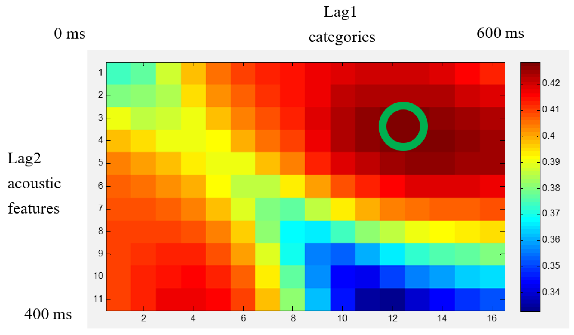
2.3. Lasso Regression

Regression analysis is a predictive modeling technique that studies the relationship between dependent variables and independent variables. This technique is commonly used for time-series models and discovering causal relationships between variables. Because emotions change over time, an emotional value is not enough to represent the dynamic emotions evoked by music. Therefore, regression analysis is applied to catch the dynamic changes in time.

Multivariable linear regression is a statistical method used to study the relationship between variables in random phenomena [35], assuming that the dependent variable Y has a linear relationship with multiple independent variables {X₁, X₂, …, X_k}. It is a multiple linear function of the independent variables, which is called a multiple linear regression model, defined as:

$$Y={\beta }_0+{\beta }_1{X}_1+{\beta }_2{X}_2+\cdots +{\beta }_k{X}_k+\mu$$

(9)

where Y is the dependent variable, X_j (j = 1, 2, …, K) are the independent variables, ${\beta }_j$ (j = 0, 1, 2, …, K) is K + 1 parameters, and μ is random errors.

The linear equation between the expected value of the dependent variable Y and the independent variables {X₁, X₂, …, X_k} is:

$$E\left(Y\right)={\beta }_0+{\beta }_1{X}_1+{\beta }_2{X}_2+\cdots +{\beta }_k{X}_k$$

(10)

For n groups of observations Y_i, X_1i, X_2i, …, X_ki (i = 1, 2, …, n), the equations are in the form:

$$Y_i={\beta }_0+{\beta }_1{X}_{1i}+{\beta }_2{X}_{2i}+\cdots +{\beta }_k{X}_{ki}+{\mu }_i,(i=1,2,\dots ,n)$$

(11)

which is:

$$\{\begin{array}{c}{Y}_1={\beta }_0+{\beta }_1{X}_{11}+{\beta }_2{X}_{21}+\cdots +{\beta }_k{X}_{k1}+{\mu }_1\\ Y_2={\beta }_0+{\beta }_1{X}_{12}+{\beta }_2{X}_{22}+\cdots +{\beta }_k{X}_{k2}+{\mu }_2\\ ⋮\\ Y_n={\beta }_0+{\beta }_1{X}_{1n}+{\beta }_2{X}_{2n}+\cdots +{\beta }_k{X}_{kn}+{\mu }_n\end{array}$$

(12)

where its matrix form is defined as:

$$Y=X\beta +\mu$$

(13)

In fact, a phenomenon is often related to multiple factors. The optimal combination of multiple independent variables is more effective and more realistic than using only one independent variable. Therefore, multiple linear regression has more practical value.

Least Absolute Shrinkage and Selection Operator (Lasso) regression is proposed by Tibshirani in 1996 to obtain a better model by constructing a first-order penalty function [36]. It puts particular variables into a model to get better performance parameters, instead of putting all the variables into the model for fitting. The complexity of the model is well controlled by the parameter λ, which could be used to avoid over-fitting [37].

$$\widehat{\beta }=argmin\left\{{\left(Y-X\beta \right)}^2+\lambda \left|\beta \right|\right\}$$

(14)

where the parameter λ is a penalty factor. The larger the λ, the stronger the punishment for the linear model with variables. Therefore, a model with fewer variables is finally obtained.

The fitting coefficient, the parameter λ, is usually defined as the smallest or standard error (SE) value. One has the best fitting effect, and the other is the better value taking into account the calculation. To obtain the best fitting result, the minimum value is considered the constraint condition in this article.

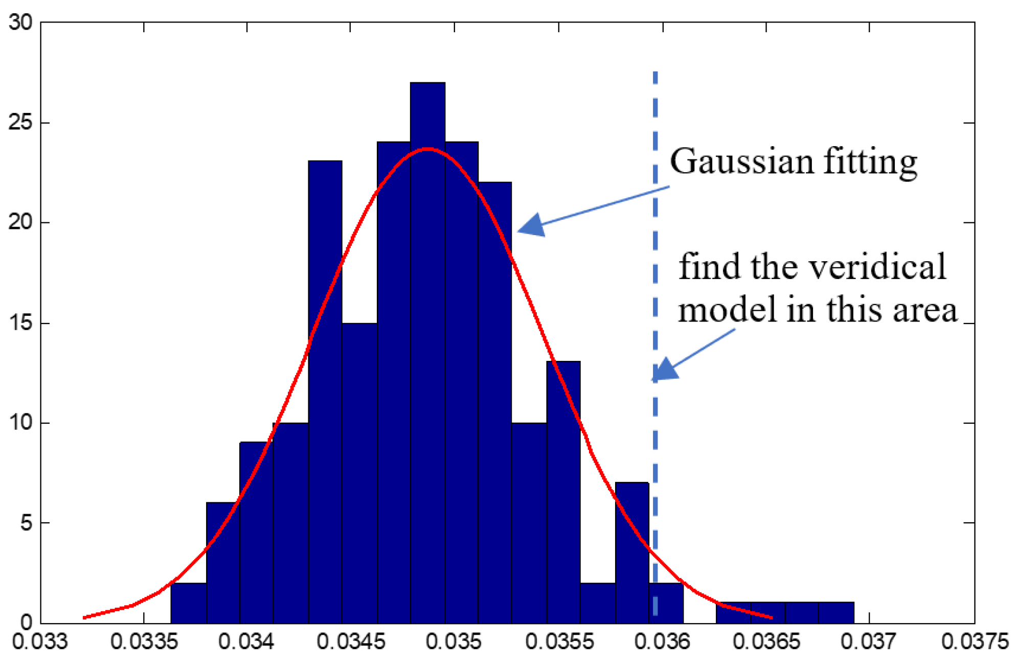
2.4. Gaussian Fitting

Gaussian fitting is a fitting method that uses the Gaussian function to approximate a set of data points. The Gaussian function is the normal distribution function. Its various parameters have a clear physical meaning, and a simple and fast calculation. The Gaussian fitting method is widely used in the measurement of analytical instruments. The Gaussian statistical model uses its probability density function (PDF) as the modeling parameter, which is the most effective feature set generation method [38].

There is a set of experimental data (x_i, y_i) (i = 1, 2, 3, …, N), which could be described by the Gaussian function, defined as:

$$y_i=y_{max}\times exp\left[-\frac{{\left(x_i-x_{max}\right)}^2}{S}\right]$$

(15)

The parameters to be estimated in Equation (15) are y_max, x_max, and S, which represent the peak value, peak position, and half-width information of the Gaussian curve, respectively. Taking the natural logarithm on both sides of the Equation (15), and using b₀, b₁, b₂ to replace the multiple items, respectively, the procedure can be matrixed as:

$$\left[\begin{array}{c}\begin{array}{c}{z}_1\\ z_2\\ ⋮\end{array}\\ z_n\end{array}\right]=\left[\begin{array}{c}\begin{array}{ccc}1& x_1& x_1^2\\ 1& x_2& x_2^2\\ ⋮& ⋮& ⋮\end{array}\\ \begin{array}{ccc}1& x_n& x_n^2\end{array}\end{array}\right]\left[\begin{array}{c}{b}_0\\ b_1\\ b_2\end{array}\right]$$

(16)

Without considering the total measurement error, it is abbreviated as:

$$Z=XB$$

(17)

According to Least-Square Principle, the generalized least-squares solution of matrix B, formed by fitting constants b₀, b₁, b₂, can be obtained as:

$$B={\left(X^{T}X\right)}^{-1}{X}^{T}Z$$

(18)

Then, the parameters to be estimated (S, x_max, and y_max) could be calculated, and the Gaussian function obtained by the Equation (15).

3. Experiments and Results

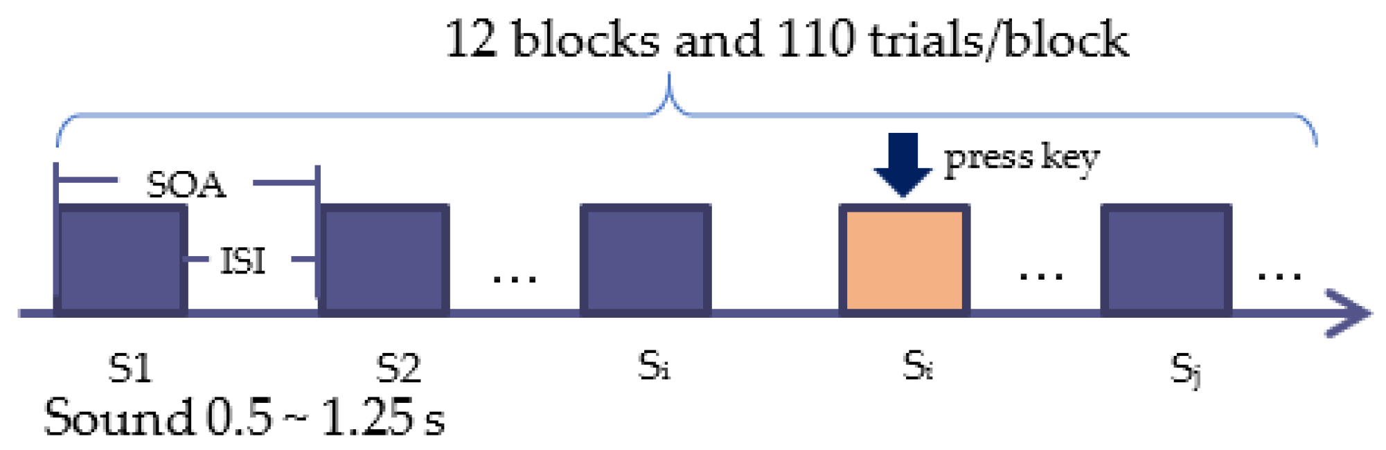
3.1. Cognitive Experiment and Data Description

To verify the method proposed in this article, a long-term auditory emotion cognition experiment was firstly designed. Music is composed of short-term notes. Therefore, 93 environment sounds were selected and played randomly, which were arranged together, and formed as a long-term sound signal. The emotional response and evaluation of sounds are essential components of human cognition. For example, people will be irritable when they hear noise, be pleased when they hear the sounds of birds, and be frightened when they hear thunder.

The experimental samples were mainly considered from two aspects: one was that short-term analysis techniques could be applied to compare with current work; and the other was to analyze the long-term brain components through the method proposed in this article. Finally, a total of 93 samples were selected with a length of 1–2 s, from 259 sounds among three emotional sound libraries, IADS2, Montreal, and MEB, based on the emotional tags.

The experimental design adopted a task-independent practical method. The entire experiment was divided into two parts: listening to the sound while collecting EEG signals; and listening to the sound and evaluating the Valence-Arousal (VA) dimensional emotions. The EEG acquisition experiment adopted the 1-back experimental paradigm, in which 20% may repeat the previous sound. The experimental process is shown in Figure 5. In addition, 51 volunteers who did not participate in the experiment evaluated the emotions of each segment online. The SAM assessment was used, which included the scores 1–9 from the three dimensions of valence, arousal, and domination.

A total of 10 volunteers (undergraduates aged between 19 and 25 years old) participated in the experiment. The experiment included 12 blocks, and each block lasted about 5 min. There was a 1-min rest between the blocks. The whole experiment was about 60 min. The EEG signal was recorded through a 128-channel EEG system (BioSemi Active Two). The sampling frequency was 1000 Hz, and the electrode arrangement was placed according to the international 10–20 system standard (shown in Figure 6). The left mastoid was used as a reference to avoid asymmetry of the left and right hemispheres.

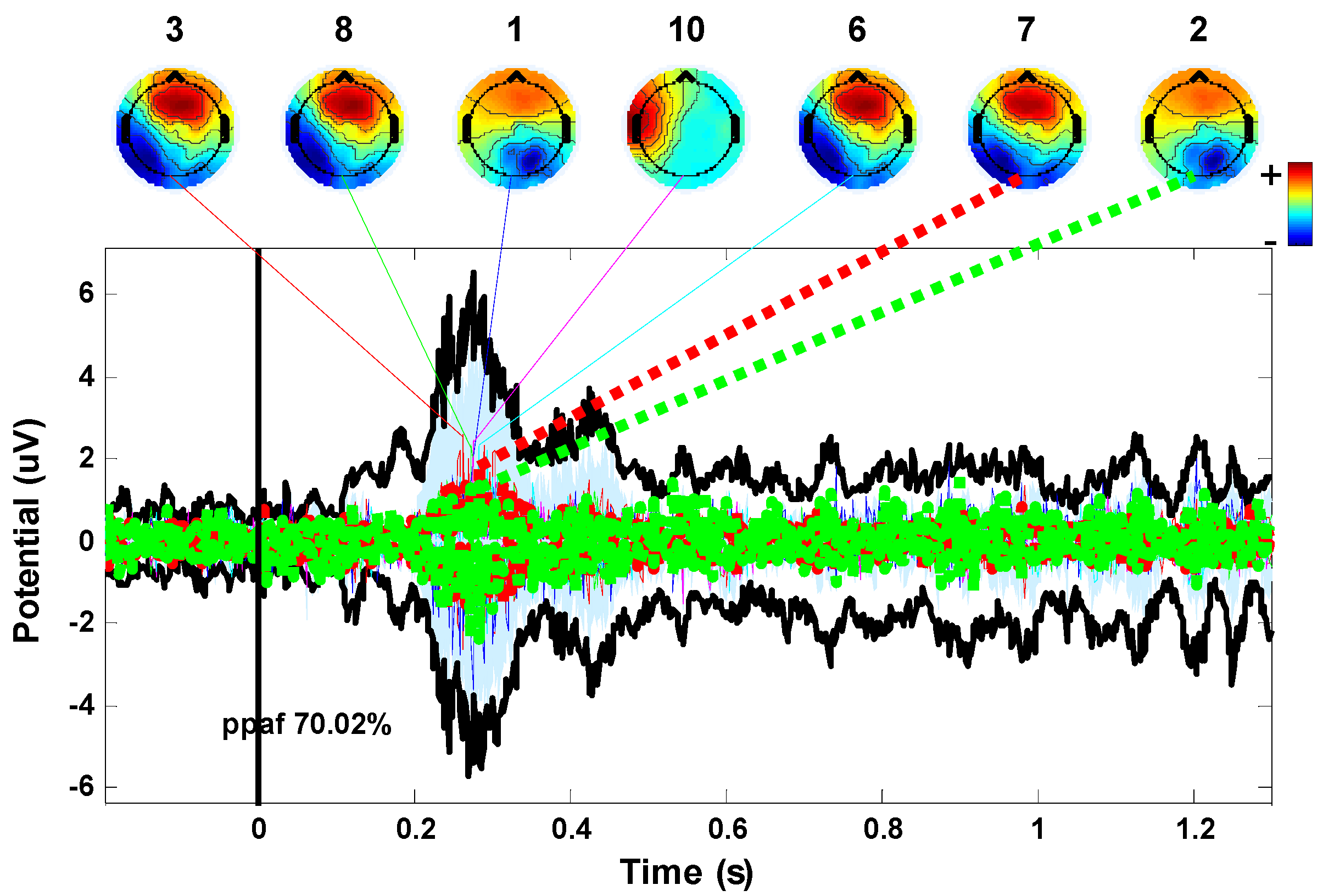
3.2. Simulation and Results

At present, the dimensional emotion model is commonly used, in which the human emotional state is formalized as a point in a two-dimensional or three-dimensional continuous space. The advantage of the dimensional model is that it can describe the fine distinction of emotional states and external physical arousal [39]. The VA dimensional model adopted in this paper was proposed by James A. Russell [40]. The model purports that emotional states are points distributed on a two-dimensional space containing Valence and Arousal. The vertical axis represents the valence, and the horizontal axis represents the activation.

(1)

Acoustic Feature Extraction

The 93 sound samples in Section 3.1 were used here, and 48 dimensional features were extracted by frames. The frame shift was set to the difference between the sampling rate of the sound signal and the EEG signal. The sound signal frame shift was set to 40 ms; the frame length was 50 ms. Based on this set of acoustic features, the stimulus feature dissimilarity matrix and the dissimilarity score of each feature were calculated. Finally, 10 acoustic features with high emotional correlation were selected, including ‘zero cross’, ‘pitch’, ‘centroid’, ‘brightness’, ‘spectral flux’, ‘roughness’, ‘tempo’, ‘loudness’, ‘spread’, and ‘roll off’, as shown in Figure 7.

The programming language was based on Matlab. The MIRtoolbox was used in the acoustic feature extraction and the EEGLAB toolbox was used in the EEG signal processing.

(2)

EEG Component Decomposition and Feature Extraction

The preprocessing was applied on the EEG signals according to the method in Section 2.2, including re-reference, removing the artifacts, and 0.5–50 Hz band-pass filtering. For calculation convenience, the EEG signals were down-sampled from 512 Hz to 100 Hz. After that, the independent components (ICs) of EEG signals were obtained by the ICA method. After removing the artifacts of ICs, a total of 428 ICs were obtained in the five frequency bands. According to Equation (5), the power spectrum density curve was calculated, and the band powers of five EEG frequency bands δ, θ, α, β, and γ were obtained. The envelopes were obtained by HT transform. As shown in Figure 8, (a) is the original EEG signal, (b) is the preprocessed EEG signal, and (c) is the HT envelope feature.

Then, the EEG features were aligned with the auditory features according to the onset time. The silent parts were filled with 0. The features were extracted from frames and spliced together to form one-dimensional time-series features, forming a long-term sound, as shown in Figure 9.

(3)

Regression Model

The multiple regression analysis was performed based on the EEG components and sound features of the time series. The independent variables were the acoustic features, and the dependent variable was the EEG component of each IC and band.

Based on the previous feature selection, supposing the optimal feature set is ${\tilde{F}}_i,i=1,2,\dots ,K$, then regression prediction equations for Valence and Arousal are established as Equation (14), where X is the feature set, Y is the average score of Valence or Arousal, and μ is the random error.

Based on the Lasso regression model, the prediction equation is solved when the fitting coefficient $\widehat{\beta }$ is the smallest.

$$\widehat{\beta }=argmin\left\{{\left(Y-\widetilde{F_i}\beta \right)}^2+\lambda \left|\beta \right|\right\}$$

(19)

Therefore, there were a total of 428 regression models and 428 fitting parameter R-squares were obtained. All the fitting parameters were plotted in order, as shown in Figure 10.

As shown in Figure 10, the horizontal axis is the dependent variable, and the curve represents the difference between the target model and the standard waveform. The ICs with the largest difference in EEG component correlation could be found. At this point, the most relevant EEG components of emotions were found: IC#41 in the alpha band, IC#1, IC#2, and IC#77 in the beta band, as shown in Figure 11. As with other auditory working memory task research [41,42], the same area on the right side of the low frequency alpha band is activated, so it is speculated that IC#41 is a working memory task.

Cong and Poikonen et al. [43,44] combined music information retrieval with spatial Fourier ICA to probe the spectral patterns of the brain network emerging from music listening. A correlation analysis was performed between EEG data and musical features (fluctuation centroid, entropy, mode, pulse clarity, and key feature). They found that an increased alpha oscillation in the bilateral occipital cortex emerged during music listening. Furthermore, musical feature time series were associated with an increased beta activation in the bilateral superior temporal gyrus. In addition, Anilesh et al. [45] used ICA to study the long-term dynamic effects of music signals on the central nervous system through EEG signal analysis. They analyzed eight components in both a pre-music state and listening to music, and found that the frontal and central lobes were affected by music. These studies confirm the effectiveness of the ICs extracted by this method [46].

4. Discussions

The goal of this article is to reveal the long-term correlation between EEG components and emotional changes. The background of this research is based on the question of how to represent and measure the brain reflection and mood changes with music in a concert hall. The existing component analysis methods are mostly for short-term EEG signals, and there are very few studies on long-term EEG signals and long-term analysis methods. Through this method, the analysis method for long-term EEG signals could be realized, the EEG components related to mood changes could be found, and the expression of long-term EEG and the comparison of long- and short-term components could be realized.

Considering the possible delay of the EEG response, an EEG signal could be offset appropriately to find the best model parameter. As shown in Figure 12, two offset parameters were considered. Lag1 was the emotional label offset parameter, and Lag2 was the acoustic feature offset parameter. The shift range of Lag1 was from 0 ms to 600 ms, and the shift range of Lag2 was from 0 ms to 400 ms. In the figure, when Lag1 = 480 ms and Lag2 = 120 ms, the fitting parameter R-square achieved the best results.

Secondly, to verify the signature of the IC with the highest correlation, we performed 200 calculations on the regression model of each subject. The histogram of the fitting parameter R-square was plotted, as shown in Figure 13.

The ICs distributed on the right side of the Gaussian fitting curve were the ICs with the highest correlation degree. Therefore, the significant brain components were IC#82 in the delta band, IC#1 and #5 in the alpha band, IC#12 in the beta band, etc. shown in Figure 14. The results are essentially consistent with studies [44,45].

5. Conclusions

Aiming at the lack of any long-term analysis method of EEG signals, a long-term EEG component analysis method based on the Lasso regression analysis is proposed in this article. To consider the temporal variation of emotions, a cognitive experiment based on environmental sounds was designed, and the EEG data of 10 volunteers were collected. In total, 48 dimensional acoustic features and 428 EEG components were extracted, representing different emotional and psychological activities. Then, a new analysis method based on the time-varying characteristics of different spaces (acoustics, physiology) was proposed. The relationship between the time-varying brain component parameters and acoustic features could be found through this method. According to the temporal relations, an optimal offset of acoustic features was found, which enabled better alignment of EEG features. After the regression analysis, the significant EEG components were found, which were in good agreement with cognitive laws.

The method proposed in this paper effectively solves the problem that existing analysis methods cannot be applied to long-term EEG components. The above work has achieved phased results and provides a basis for the study of auditory emotional cognition. In the future, more in-depth research will be carried out on auditory emotional cognition and calculation methods to explore the universal principles of affective computing. When experimental data is adequately accumulated, the classification model can be carried out. Then, an automatic emotion prediction and recognition system with an auditory and physiological response could be built.

References

1. Picard, R.W. Affective Computing; MIT Press: Cambridge, MA, USA, 1997; pp. 71–73. [Google Scholar]
2. Paszkiel, S. Control based on brain-computer interface technology for video-gaming with virtual reality techniques. J. Autom. Mob. Robot. Intell. Syst. 2016, 10, 3–7. [Google Scholar]
3. Juslin, P.N.; Västfjäll, D. Emotional responses to music: The need to consider underlying mechanisms. Behav. Brain Sci. 2008, 31, 751. [Google Scholar] [CrossRef] [Green Version]
4. Bo, H.; Li, H.; Wu, B.; Ma, L.; Li, H. Brain Cognition of Musical Features Based on Automatic Acoustic Event Detection. In Proceedings of the International Conference on Multimedia Information Processing and Retrieval, Shenzhen, China, 6–8 August 2020; IEEE: New York, NY, USA, 2020; pp. 382–387. [Google Scholar]
5. Chen, X.; Yang, D. Research Progresses in Music Emotion Recognition. J. Fudan Univ. 2017, 56, 136–148. [Google Scholar]
6. Schaefer, H. Music-evoked emotions—Current studies. Front. Neurosci. 2017, 11, 600. [Google Scholar] [CrossRef]
7. Daly, I.; Nicolaou, N.; Williams, D.; Hwang, F.; Kirke, A.; Miranda, E.; Nasuto, S.J. Neural and physiological data from participants listening to affective music. Sci. Data 2020, 7, 177. [Google Scholar] [CrossRef]
8. Madsen, J.; Sand Jensen, B.O.R.; Larsen, J. Modeling temporal structure in music for emotion prediction using pairwise comparisons. In Proceedings of the International Society of Music Information Retrieval Conference, Taipei, Taiwan, 27–31 October 2014. [Google Scholar]
9. Saari, P.; Eerola, T.; Fazekas, G.O.R.; Barthet, M.; Lartillot, O.; Sandler, M.B. The role of audio and tags in music mood prediction: A study using semantic layer projection. In Proceedings of the International Society for Music Information Retrieval Conference, Curitiba, Brazil, 4–8 November 2013; pp. 201–206. [Google Scholar]
10. Han, W.; Li, H.; Han, J. Speech emotion recognition with combined short and long term features. Tsinghua Sci. Technol. 2007, 48, 708–714. [Google Scholar]
11. Hu, L.; Zhang, Z. EEG Signal Processing and Feature Extraction, 1st ed.; Science Press: Beijing, China, 2020. [Google Scholar]
12. Yu, B.; Wang, X.; Ma, L.; Li, L.; Li, H. The Complex Pre-Execution Stage of Auditory Cognitive Control: ERPs Evidence from Stroop Tasks. PLoS ONE 2015, 10, e0137649. [Google Scholar] [CrossRef]
13. Luck, S.J. An Introduction to the Event-Related Potential Technique; MIT Press: Cambridge, MA, USA, 2014. [Google Scholar]
14. Poikonen, H.; Alluri, V.; Brattico, E.; Lartillot, O.; Tervaniemi, M.; Huotilainen, M. Event-related brain responses while listening to entire pieces of music. Neuroscience 2016, 312, 58–73. [Google Scholar] [CrossRef]
15. Welch, P.D. The use of fast Fourier transform for the estimation of power spectra: A method based on time averaging over short, modified periodograms. IEEE Trans. Audio Electroacoust. 1967, 15, 70–73. [Google Scholar] [CrossRef] [Green Version]
16. Bo, H. Research on Affective Computing Methods Based on Auditory Cognitive Principles. Ph.D. Thesis, Harbin Institute of Technology, Harbin, China, 2019. [Google Scholar]
17. Wright, J.J.; Kydd, R.R.; Sergejew, A.A. Autoregression models of EEG. Biol. Cybern. 1990, 62, 201–210. [Google Scholar] [CrossRef]
18. Zhang, Y.; Zhang, S.; Ji, X. EEG-based classification of emotions using empirical mode decomposition and autoregressive model. Multimed. Tools Appl. 2018, 77, 26697–26710. [Google Scholar] [CrossRef]
19. Li, H.; Li, H.; Ma, L. Long-term Music Emotion Research Based on Dynamic Brain Network. J. Fudan Univ. Nat. 2020, 59, 330–337. [Google Scholar]
20. Murugappan, M.; Rizon, M.; Nagarajan, R.; Yaacob, S.; Zunaidi, I.; Hazry, D. EEG feature extraction for classifying emotions using FCM and FKM. Int. J. Comput. Commun. 2007, 1, 21–25. [Google Scholar]
21. Lin, Y.; Wang, C.; Jung, T.; Wu, T.; Jeng, S.; Duann, J.; Chen, J. EEG-based emotion recognition in music listening. IEEE. Trans. Biomed. Eng. 2010, 57, 1798–1806. [Google Scholar] [PubMed]
22. Petrantonakis, P.C.; Hadjileontiadis, L.J. Adaptive emotional information retrieval from EEG signals in the time-frequency domain. IEEE Trans. Signal Process. 2012, 60, 2604–2616. [Google Scholar] [CrossRef]
23. Tripathi, S.; Acharya, S.; Sharma, R.D.; Mittal, S.; Bhattacharya, S. Using deep and convolutional neural networks for accurate emotion classification on DEAP dataset. In Proceedings of the Twenty-ninth Innovative Applications of Artificial Intelligence Conference, San Francisco, CA, USA, 6–9 February 2017; pp. 4746–4752. [Google Scholar]
24. Giannakakis, G.; Grigoriadis, D.; Giannakaki, K.; Simantiraki, O.; Roniotis, A.; Tsiknakis, M. Review on psychological stress detection using biosignals. IEEE Trans. Affect. Comput. 2019. [Google Scholar] [CrossRef]
25. Xie, Y.; Liang, R.; Liang, Z.; Huang, C.; Zou, C.; Schuller, B. Speech emotion classification using attention-based LSTM. IEEE/ACM Trans. Audio Speech Lang. Process. 2019, 27, 1675–1685. [Google Scholar] [CrossRef]
26. Levy, D.A.; Granot, R.; Bentin, S. Neural sensitivity to human voices: ERP evidence of task and attentional influences. Psychophysiology 2003, 40, 291–305. [Google Scholar] [CrossRef]
27. Klug, M.; Gramann, K. Identifying key factors for improving ICA-based decomposition of EEG data in mobile and stationary experiments. Eur. J. Neurosci. 2020. [Google Scholar] [CrossRef]
28. Jung, T.; Makeig, S.; Westerfield, M.; Townsend, J.; Courchesne, E.; Sejnowski, T.J. Removal of eye activity artifacts from visual event-related potentials in normal and clinical subjects. Clin. Neurophysiol. 2000, 111, 1745–1758. [Google Scholar] [CrossRef]
29. Li, Y.; Qiu, Y.; Zhu, Y. EEG Signal Analysis Method and Its Application; Science Press: Beijing, China, 2009. [Google Scholar]
30. Hettich, D.T.; Bolinger, E.; Matuz, T.; Birbaumer, N.; Rosenstiel, W.; Spüler, M. EEG responses to auditory stimuli for automatic affect recognition. Front. Neurosci. 2016, 10, 244. [Google Scholar] [CrossRef]
31. Masuda, F.; Sumi, Y.; Takahashi, M.; Kadotani, H.; Yamada, N.; Matsuo, M. Association of different neural processes during different emotional perceptions of white noise and pure tone auditory stimuli. Neurosci. Lett. 2018, 665, 99–103. [Google Scholar] [CrossRef]
32. Raheel, A.; Anwar, S.M.; Majid, M. Emotion recognition in response to traditional and tactile enhanced multimedia using electroencephalography. Multimed. Tools Appl. 2019, 78, 13971–13985. [Google Scholar] [CrossRef]
33. Johansson, M. The Hilbert Transform. Ph.D. Thesis, Växjö University, Växjö, Suecia, 1999. [Google Scholar]
34. Huang, N.E. Hilbert-Huang Transform and Its Applications, 1st ed.; World Scientific Publishing: Singapore, 2014. [Google Scholar]
35. Gifi, A. Nonlinear Multivariate Analysis; Wiley-Blackwell: New York, NY, USA, 1990. [Google Scholar]
36. Tibshirani, R. Regression shrinkage and selection via the lasso. J. R. Stat. Soc. 1996, 58, 267–288. [Google Scholar] [CrossRef]
37. Meziani, A.; Djouani, K.; Medkour, T.; Chibani, A. A Lasso quantile periodogram based feature extraction for EEG-based motor imagery. J. Neurosci. Methods 2019, 328, 108434. [Google Scholar] [CrossRef] [PubMed]
38. Chowdhury, T.T.; Fattah, S.A.; Shahnaz, C. Seizure activity classification based on bimodal Gaussian modeling of the gamma and theta band IMFs of EEG signals. Biomed. Signal Process. Control 2021, 64, 102273. [Google Scholar] [CrossRef]
39. Li, H.; Chen, J.; Ma, L.; Bo, H.; Xu, C.; Li, H. Dimensional Speech Emotion Recognition Review. J. Softw. 2020, 31, 2465–2491. [Google Scholar]
40. Feldman, L.A. Valence focus and arousal focus: Individual differences in the structure of affective experience. J. Pers. Soc. Psychol. 1995, 69, 153–166. [Google Scholar] [CrossRef]
41. Yu, X.; Chen, Y.; Luo, T.; Huang, X. Neural oscillations associated with auditory duration maintenance in working memory in tasks with controlled difficulty. Front. Psychol. 2020, 11, 545935. [Google Scholar] [CrossRef]
42. Billig, A.J.; Herrmann, B.; Rhone, A.E.; Gander, P.E.; Nourski, K.V.; Snoad, B.F.; Kovach, C.K.; Kawasaki, H.; Howard, M.A., 3rd; Johnsrude, I.S. A sound-sensitive source of alpha oscillations in human non-primary auditory cortex. J. Neurosci. 2019, 39, 8679–8689. [Google Scholar] [CrossRef]
43. Zhu, Y.; Zhang, C.; Poikonen, H.; Toiviainen, P.; Huotilainen, M.; Mathiak, K.; Ristaniemi, T.; Cong, F. Exploring Frequency-Dependent Brain Networks from Ongoing EEG Using Spatial ICA During Music Listening. Brain Topogr. 2020, 33, 289–302. [Google Scholar] [CrossRef] [PubMed] [Green Version]
44. Mei, J.; Wang, X.; Liu, Y.; Li, J.; Liu, K.; Yang, Y.; Cong, F. The Difference of Music Processing among Different State of Consciousness: A Study Based on Music Features and EEG Tensor Decomposition. Chin. J. Biomed. Eng. 2021, 40, 257–265. [Google Scholar]
45. Dey, A.; Palit, S.K.; Bhattacharya, D.K.; Tibarewala, D.N.; Das, D. Study of the effect of music on central nervous system through long term analysis of EEG signal in time domain. Int. J. Eng. Sci. Emerg. Technol. 2013, 5, 59–67. [Google Scholar]
46. Yang, W.; Wang, K.; Zuo, W. Fast neighborhood component analysis. Neurocomputing 2012, 83, 31–37. [Google Scholar] [CrossRef]
Figure 1. Schematic diagram of ERP analysis method. The curve in the figure is ERP induced by emotional sounds. Seven EEG components contribute the most.
Algorithms 14 00271 g001
Figure 2. The process of the long-term EEG component analysis method proposed in this article.
Algorithms 14 00271 g002
Figure 3. The similarity matrices of the same feature (zero crossing) were calculated respectively by using (a) Euclidean distance, (b) Mahalanobis distance, and (c) Cosine similarity. A dark color means similar and a bright color means dissimilar. The sum value of dissimilarity by cosine was higher than the euclidean and mahalanobis distances.
Algorithms 14 00271 g003
Figure 4. The process of EEG component decomposition and feature extraction.
Algorithms 14 00271 g004
Figure 5. The experimental flow of sound-induced emotion.
Algorithms 14 00271 g005
Figure 6. Electrode location distribution.
Algorithms 14 00271 g006
Figure 7. Acoustic features for a specific sound. (The horizontal axis represents sampling points, and the vertical axis represents the value of features).
Algorithms 14 00271 g007
Figure 8. The envelope feature by Hilbert transformation. (a) is the original EEG signal, (b) is the preprocessed EEG signal, and (c) is the HT envelope feature.
Algorithms 14 00271 g008
Figure 9. Acoustic and EEG features aligned. (The acoustic features are extracted from frames and spliced together to form one-dimensional time-series features. Then, they are used as independent variables to estimate each EEG component).
Algorithms 14 00271 g009
Figure 10. The R-squares of 428 regression models. (The horizontal axis represents the number of regression equations, and the vertical axis represents the value of R-square).
Algorithms 14 00271 g010
Figure 11. The most relevant emotion-related long-term brain components. (a) is the IC#41 in the alpha band, (b) is the IC#1 in the beta band.
Algorithms 14 00271 g011
Figure 12. The regression effects by offset parameters of acoustic features and labels.
Algorithms 14 00271 g012
Figure 13. The result of Gaussian Fitting.
Algorithms 14 00271 g013
Figure 14. The significant brain components selected by the Gaussian fitting. (a,b) are the IC#1 and #5 in the alpha band, and (c) is the IC#12 in the beta band.
Algorithms 14 00271 g014
Publisher’s Note: MDPI stays neutral with regard to jurisdictional claims in published maps and institutional affiliations.