A Real-Time Network Traffic Classifier for Online Applications Using Machine Learning

Abstract

The increasing ubiquity of network traffic and the new online applications’ deployment has increased traffic analysis complexity. Traditionally, network administrators rely on recognizing well-known static ports for classifying the traffic flowing their networks. However, modern network traffic uses dynamic ports and is transported over secure application-layer protocols (e.g., HTTPS, SSL, and SSH). This makes it a challenging task for network administrators to identify online applications using traditional port-based approaches. One way for classifying the modern network traffic is to use machine learning (ML) to distinguish between the different traffic attributes such as packet count and size, packet inter-arrival time, packet send–receive ratio, etc. This paper presents the design and implementation of NetScrapper, a flow-based network traffic classifier for online applications. NetScrapper uses three ML models, namely K-Nearest Neighbors (KNN), Random Forest (RF), and Artificial Neural Network (ANN), for classifying the most popular 53 online applications, including Amazon, Youtube, Google, Twitter, and many others. We collected a network traffic dataset containing 3,577,296 packet flows with different 87 features for training, validating, and testing the ML models. A web-based user-friendly interface is developed to enable users to either upload a snapshot of their network traffic to NetScrapper or sniff the network traffic directly from the network interface card in real time. Additionally, we created a middleware pipeline for interfacing the three models with the Flask GUI. Finally, we evaluated NetScrapper using various performance metrics such as classification accuracy and prediction time. Most notably, we found that our ANN model achieves an overall classification accuracy of 99.86% in recognizing the online applications in our dataset.

1. Introduction

Network traffic analysis is the process of recognizing user applications, networking protocols, and communication patterns flowing through the network [1]. Traffic analysis is useful for identifying security threats, intrusion detection, server performance deterioration, configuration errors, and latency problems in some network components [2]. The rapid evolution of new online applications, as well as the ubiquitous deployment of mobile and IoT devices [3], have dramatically increased the complexity and diversity of network traffic analysis. Moreover, the new security requirements in modern networks, including packet encryption and port obfuscation, have elevated extra challenges in classifying network traffic [4].

Despite the importance, the traditional network traffic classification approaches can only recognize user applications that are running over static well-known network ports such as FTP, SSH, HTTP, SMTP, etc. However, most online user applications use dynamic ports, virtual private networks, and encrypted tunnels [5]. Furthermore, these applications are transported over HTTPS connections and have applied security protocols (e.g., SSH and SSL) for ensuring QoS provisioning, security, and privacy. This makes it very challenging for traditional port-based approaches to recognize such applications.

Machine learning (ML), including deep learning (DL), has already enabled game-changing traffic analysis capabilities by providing the ability to understand network traffic behavior and patterns, and distinguish between benign and abnormal traffic [2,6,7]. For instance, ML-based cybersecurity approaches have made significant contributions in detecting various types of attacks [8], such as multi-class distinction of Distributed Denial of Service (DDOS) attacks, DoS Hulk, DoS GoldenEye, Heartbleed, Bot, PortScan, and Web attacks. Imagine a user-friendly network traffic flow classifier that network administrators can use to identify the different types of online applications flowing their networks with high accuracy. Such systems would help them to perform administrative decisions, and detect malicious traffic and secure users’ data.

This paper presents NetScrapper, a lightweight ML-powered traffic flow classifier for online applications, which can be deployed on-site at the network edge. We compared three different ML models, namely K-Nearest Neighbors (KNN), Random Forest (RF), and Artificial Neural Network (ANN), for classifying the most popular 53 online user applications, including Amazon, Youtube, Google, Twitter, and many others. NetScrapper uses a network traffic dataset that consists of more than 3.5 M flow packets with different 78 features for training, validating, and testing the KNN, RF, and ANN models.

We developed a web-based interface using Python Flask Framework [9], which enables users to either upload a snapshot of their traffic history or capture the traffic flow directly from the network interface card in real time. The GUI displays the confidence percentage and classification time taken to classify the traffic flow. The web application runs on top of KNN, RF, and ANN models. To enable seamless interfacing between the three ML models and the Flask GUI, we built a middleware pipeline that orchestrates the coordination between the different components of the traffic classifier.

The contributions of this paper are fourfold. First, we propose NetScrapper, an AI-powered network classifier for real-time flow streams that can help network administrators to monitor their network performance and detect any suspicious traffic circulating their networks. NetScrapper can be deployed on networking devices at the network edge with high prediction accuracy and low response time. Second, we carried out several sets of experiments for evaluating the classification accuracy and performance of three different ML models (i.e., ANN, RF, and KNN) implemented as part of NetScrapper. Third, we developed a user-friendly interface on top of the three ML models to allow users to interact with the network classifier conveniently. Fourth, the system is designed to be generic, making it applicable to different fields requiring real-time inference at the network edge with offline generated ML models.

The rest of the paper is organized as follows: Section 2 presents related work. Section 3 and Section 4 present the design and prototype implementation of NetScrapper, respectively. Section 5 experimentally evaluates NetScrapper in terms of classification time and accuracy. Finally, Section 6 summarizes the results of this work.

2. Related Work

The evolution of traffic flow classification has gone through three stages: port-based, payload-based, and flow-based statistical characteristics. Port-based approaches assume that online applications consistently use well-known TCP or UDP port numbers; however, the emergence of port camouflage, random port, and tunneling technology makes these port-based approaches lose productiveness quickly [10]. Payload-based methods, also called Deep Packet Inspection (DPI) techniques, depend on inspecting both the packet header and data parts to determine any non-compliance to transportation protocols or the existence of spam, viruses, or intrusions to take preventative actions by blocking, re-routing, or logging the packet accordingly. However, payload-based approaches cannot deal with encrypted traffic as it needs to match packet content to static routing rules [2]. Additionally, DPI approaches tend to have high computational overhead, which precludes its real-time usage in mission-critical security tasks [11].

In this paper, we focus on the flow-based approach that relies on network traffic statistical characteristics using ML algorithms [7]. Flow-based techniques help network administrators and security personnel to monitor both ingress and egress traffic communicated from/to external networks to/from their enterprise networks [11]. Furthermore, statistical characterization helps minimize the false positives in automated intrusion detection systems [5]. This section provides an overview of the most important network traffic classification methods. In particular, we focus on statistical and machine learning approaches.

Deep Packet [2] is an example of a DL-based scheme for traffic flow classification that integrates both feature extraction and classification phases into one system. Deep Packet focuses on traffic characterization, including encrypted traffic, to identify end-user applications (e.g., BitTorrent and Skype). The proposed method uses two DL models, namely Stacked Autoencoder (SAE) and Convolution Neural Network (CNN), to classify the encrypted traffic across VPN networks. Experimental results showed that the CNN model achieved an overall classification accuracy of 94% in recognizing the flow traffic. However, Deep Packet can only detect a limited range of online applications due to the relatively small training dataset.

In the field of cybersecurity, Rezaei et al. [1] proposed a multi-task learning framework for network traffic classification. The proposed framework can predict the bandwidth requirement and duration of the traffic flow generated for online applications. The authors claim that their framework can achieve a high classification accuracy of user applications using easily obtainable data samples for bandwidth and duration, thus eliminating the need for a sizeable labeled traffic dataset. Experimental evaluation was conducted using ISCX and QUIC public datasets showed the efficacy of the proposed approach.

Another DL-based network encrypted traffic classifier and intrusion detection system, called Deep-Full-Range (DFR), was proposed in [5]. DFR can use CNN, SAE, and Long Short-Term Memory (LSTM) models to classify encrypted and malware traffic without human intervention. DFR was compared to some state-of-the-art approaches using two public datasets. Experimental results showed that DFR slightly outperforms these approaches in terms of F1 score and storage resource requirements. However, DFR relies on manual feature extraction to train the DL models, limiting the system’s usability on a large scale.

Focusing on real-world network traffic, Hardegen et al. [7] proposed a processing pipeline for flow-based traffic classification using machine learning. The proposed system is trained to predict the characteristics of real-world traffic flows (e.g., throughput and duration) from a campus network. The pipeline has preprocessing and anonymization modules that can protect sensitive user information circulating the campus network. A visualization module was developed to illustrate the network traffic data visually to system users. Although this work seems promising, no experimental evaluation was conducted to assess the proposed system’s performance and scalability.

Interesting work was presented in [10] for online classification of user activities using machine learning on network traffic. The authors proposed a system for classifying user activities from network traffic using both supervised and unsupervised learning. The proposed method uses users’ behavior exhibited over the network to classify their activities within a given time window. An RF model was trained with features extracted from the network and transport layer headers in the traffic flows. The RF model achieved a prediction rate of 97.37% in recognizing the user activities over short temporal windows. However, this system assumes that users are performing a single activity anytime, thereby obtaining one label for each temporal window. This excludes simultaneous activities performed by one user, which is an essential requirement in modern networks.

In summary, most of the existing work on statistical [1,7,10] and ML-based traffic classification [2,5,11] focus on extracting low handcrafted features from the traffic flow, which always depends on the domain experts’ experience. These flow features must also be up-to-date to cope with the rapidly changing world of new online applications [3]. Moreover, most of the surveyed DL-based models are designed to work offline, which is not appropriate for real-time network traffic analysis. Furthermore, to the best of our knowledge, none of the current ML-based approaches can be deployed on-site at the network edge with a user-friendly interface, which precludes minimizing the communication delays and enhancing the user experience in using the system.

3. System Design

This section presents the design of NetScrapper, including the system architecture, dataset, and the three ML models. In the rest of this section, we discuss these parts separately.

3.1. Architecture

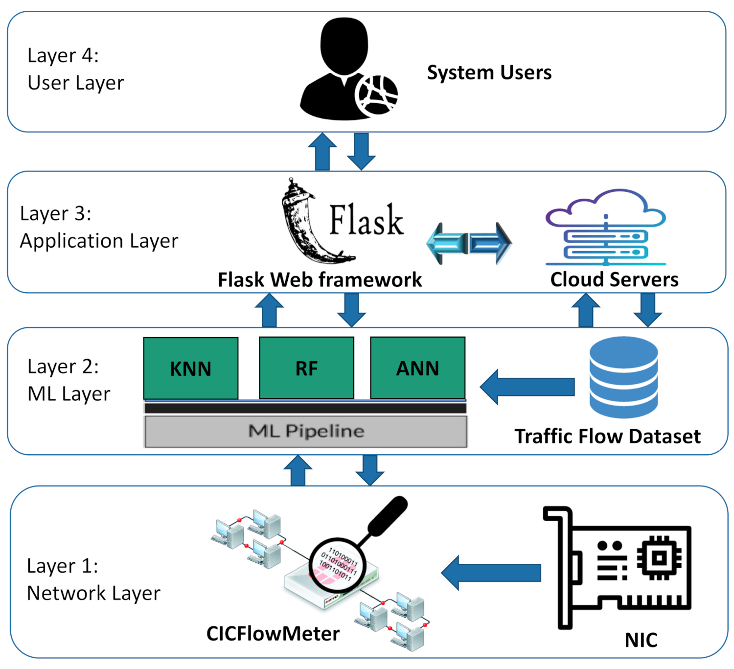
As illustrated in Figure 1, the run-time system for NetScrapper is organized with parts executing on the network and application layers. Layer 1 shows that live traffic flows are extracted from the Network Interface Card (NIC), stored, and preprocessed in real time. The traffic stream is then fed into CICFlowMeter [12], an open-source tool that extracts the time-related features from the network flow stream to train the ML models. CICFlowMeter can generate these features from bidirectional flows, purifying attributes from an existing feature set, and control the duration of flow timeout for both TCP and UDP protocols.

Layer 2 describes the machine learning models used in NetScrapper, including the KNN, RF, and ANN models. It also shows the Ml pipeline, which runs underneath the three ML models. The pipeline automates the ML workflow by enabling live traffic flows to be transformed and correlated into each ML model to achieve the desired classification outputs. It also works as a coordination interface between the Flask GUI and the ML models. The ML pipeline transformed our ML workflows into independent, reusable, modular components that can then be pipelined together to build a more efficient and simplified real-time traffic classifier. Layer 3 illustrates the web-based interface of NetScrapper running on the cloud server. We used Python Flask Framework to develop a user-friendly web application that enables users (shown in layer 4) to interact with the system.

3.2. Dataset

We collected more than labeled 3.5 M flow packets with different 78 feature attributes such as header length, flow duration, flow IAT mean, down–up ratio, segment size, acknowledge flag count, etc. As show in

Table 1. Attribute categories of our traffic flow dataset.

Category	Attributes
Subflow descriptors (4)	Subflow Fwd Packets; Subflow Fwd Bytes; Subflow Bwd Packets; Subflow Bwd Bytes
Header descriptors (5)	Fwd Header Length; Bwd Header Length; Average Packet Size; Fwd Header Length
Network identifiers (7)	FlowID; Source IP; Source Port; Destination IP; Destination Port; Protocol; Timestamp
Flow timers (8)	Active Mean; Active Std; Active max; Active min; Idle Mean; Idle std; Idle max; Idle min
Flag Features (12)	Fwd PSH flags; Bwd PSH flags; Fwd URG flags; Bwd URG flags; FIN Flag Count; SYN Flag Count; RST Flag Count; PSH Flag Count; ACK Flag Count; URG Flag Count; CWE Flag Count; ECE Flag Count
Interarrival times (15)	Flow Duration; Flow IAT Mean; Flow IAT std; Flow IAT Max; Flow IAT Min; Fwd IAT Total; Fwd IAT Mean; Fwd IAT Std; Fwd IAT Max; Fwd IAT Min; Bwd IAT Total; Bwd IAT Mean; Bwd IAT Std; Bwd IAT Max; Bwd IAT Min
Flow descriptors (36)	Total Fwd Packets; Total Bwd Packets; Total Length of Fwd Packets; Total Length of Bwd Packets; Fwd Packet Length Max; Fwd Packet Length Max; Fwd Packet Length Min; Fwd Packet Length Mean; Fwd Packet Length Std; Bwd Packet Length Max; Bwd Packet Length Min; Bwd Packet Length Mean; Bwd Packet Length Std; Flow Bytes S; Flow Packets S; Min Packet Length; Max Packet Length; Packet Length Mean; Packet Length Std; Packet Length Variance; Down Up Ratio; Avg Fwd Segment Size; Avg Bwd Segment Size; Fwd Avg Bytes Bulk; Fwd Avg Packets Bulk; Fwd Avg Bulk Rate; Bwd Avg Bytes Bulk; Bwd Avg Packets Bulk; Bwd Avg Bulk Rate; Init Win bytes forward; Init Win bytes backward; act data pkt fwd; min seg size forward; Label; L7Protocol; ProtocolName

, we categorized these attributes into seven main attribute categories, namely subflow descriptors (4 attributes), header descriptors (5 attributes), network identifiers (7 attributes), flow timers (8 attributes), flag features (12 attributes), interarrival times (15 attributes), and flow descriptors (36 attributes).

Table 2. The number of samples used in the training phase across the online application classes.

Class #	Application Name	Number of Samples
1	GOOGLE	959,110
2	HTTP	683,734
3	HTTP_PROXY	623,210
4	SSL	404,883
5	HTTP_CONNECT	317,526
6	YOUTUBE	170,781
7	AMAZON	86,875
8	MICROSOFT	54,710
9	GMAIL	40,260
10	WINDOWS_UPDATE	34,471
11	SKYPE	30,657
12	FACEBOOK	29,033
13	DROPBOX	25,102
14	YAHOO	21,268
15	TWITTER	18,259
16	CLOUDFLARE	14,737
17	MSN	14,478
18	CONTENT_FLASH	8589
19	APPLE	7615
20	OFFICE_365	5941
21	WHATSAPP	4593
22	INSTAGRAM	2415
23	WIKIPEDIA	2025
24	MS_ONE_DRIVE	1748
25	DNS	1695
26	IP_ICMP	1631
27	NETFLIX	1560
28	APPLE_ITUNES	1287
29	SPOTIFY	1269
30	APPLE_ICLOUD	1200
31	EBAY	1192
32	SSL_NO_CERT	856
33	GOOGLE_MAPS	807
34	EASYTAXI	705
35	TEAMVIEWER	527
36	HTTP_DOWNLOAD	516
37	MQTT	302
38	TOR	276
39	FTP_DATA	251
40	UBUNTUONE	249
41	NTP	135
42	SSH	102
43	EDONKEY	95
44	WAZE	79
45	DEEZER	74
46	UNENCRYPED_JABBER	45
47	CITRIX_ONLINE	38
48	TIMMEU	34
49	UPNP	34
50	TELEGRAM	33
51	FTP_CONTROL	25
52	TWITCH	24
53	H323	21

shows the number of samples used in the training phase of the ML models across the 53 online popular applications, including Google, Youtube, Amazon, Microsoft, Dropbox, Facebook, Twitter, Instagram, Netflix, Apple, Skype, etc. The dataset was collected from different sources such as Kaggle [13], Wireshark analysis [14], and other sources. Our dataset is divided into three parts: training, validation, and testing. The number of samples in each phase is determined based on the fine-tuned hyperparameters and structure of the ML models. Specifically, 70% of the dataset is allocated for the training phase, while the remaining 30% is equally partitioned between the validation and testing phases.

We applied a series of preprocessing transformations to the training dataset to increase the training accuracy and minimize the training loss of the ML models. This had a better effect on learning the 53 classes more effectively and increased our ML models’ stability. First, we used CICFlowmeter to store the traffic stream into PCAP files temporarily. Then, the Scapy tool [15] is used to manipulate the captured packets in these PCAP files to weaken the influence of the network noise factor and eliminate the incomplete records during the training process. The result data are stored in CSV files. Second, the ML pipeline performs a deep packet inspection on these CSV files to extract the feature attributes, including the application protocol (layer 7 in the TCP/IP stack), source IP address, source port, destination IP address, destination port, etc.

We also altered the Ethernet header for some packets in our dataset because the transport layer segments in the TCP and UDP protocols vary in header length. For instance, the TCP and UDP packets’ header lengths are 20 and 8 bytes, respectively. Therefore, we inserted zeros to the end of the UDP protocol’s packet headers to equalize all packets’ length in our dataset. These preprocessing and feature extraction steps are summarized in Algorithm 1.

Algorithm 1 Preprocessing and Feature Extraction Algorithm

1: procedure Preprocess Training Dataset 2: Input: Raw Dataset ($RD$) 3: Output 1: Preprocessed Dataset ($PD$) 4: Output 2: Feature Attributes ($FT$) 5: /* generate the PCAP files */ 6: PCAP-List = generatePCAP($RD$); 7: /* purify the PCAP files */ 8: for each PCAP file in PCAP-List do 9:   /* remove noise and incomplete traffic packets */ 10:   CSV-File = purifyDataset(file); 11:   /* Standardize the length of packets’ headers */ 12:   packetList = alterPacketHeader(CSV-File); 13:   $PD$.add(packetList); 14:   /* extract the feature vector from each packet */ 15:   v = getFeatureVector(packetList); 16:   $FT$.add(v); 17: end for 18: return $PD$ and $FT$;

The preprocessing operation was customized for each ML model based on its hyperparameters and structure. Furthermore, the size of the training set and the number of feature attributes were reduced from 16,545,768 to 3,577,296 packet flows and from 86 to 78, respectively. We eliminated the following feature attributes from the dataset because they could be derived from other exciting attributes: URG Flag Count, CWE Flag Count, Flow Bytes S, Subflow Fwd Bytes, Subflow Bwd Bytes, Bytes Bulk, Bwd Avg Bytes Bulk, Init Win bytes forward, Init Win bytes backward.

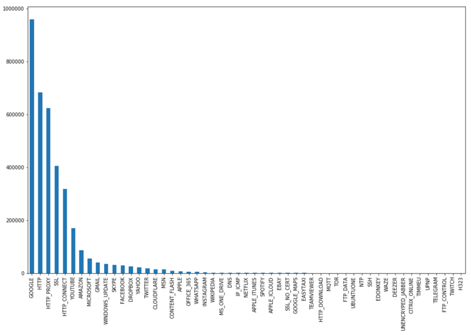
Figure 2 gives a general overview of the number of samples in our dataset across the 53 classes after the preprocessing stage.

We had to normalize the range of values of the feature attributes in the dataset before training the ML models. This step was necessary because all dimensions of feature vectors extracted from input traffic data should be in the same range. This made the convergence of our ML models faster during the training phase. Statistical normalization (Z-transformation) was implemented by subtracting the input mean value $\mu$ from each attribute’s value $I\left(i\right)$, and then dividing the result by the standard deviation $\sigma$ of the input feature vector. The distribution of the output traffic values would resemble a Gaussian curve centered at zero. We used the following formula to normalize each feature vector in our training set:

$$O\left(i\right)=\frac{I\left(i\right)-\mu }{\sigma }$$

(1)

where I and O are the input and output feature vectors, respectively; and i is the current feature vector’s index to be normalized.

3.3. ML Models

3.3.1. ANN Structure

We trained a feed-forward ANN model with 2 hidden layers, one input layer and one output layer. $I=[i_1,i_2,\dots ,i_r]$ and $O=[o_1,o_2,\dots ,o_h]$ represent the input and output vectors, respectively, where r represents the number of elements in the input feature set and h is the number of classes. The main objective of the network is to learn a compressed representation of the dataset. In other words, it tries to approximately learns the identity function F, which is defined as:

$$F_{W,B}\left(I\right)\simeq I$$

(2)

where W and B are the whole network weights and biases vectors.

A log sigmoid function is selected as the activation function f in the hidden and output neurons. The log sigmoid function s is a special case of the logistic function in the t space, which is defined by the following formula:

$$s\left(t\right)=\frac{1}{1+e^{-}t}$$

(3)

The weights of the ANN network create the decision boundaries in the feature space, and the resulting discriminating surfaces can classify complex boundaries. During the training process, these weights are adapted for each new training image. In general, feeding the ANN model with more samples can recognize the online applications more accurately. We used the back-propagation algorithm, which has a linear time computational complexity, for training the ANN model.

The input value $\Theta$ going into a node i in the network is calculated by the weighted sum of outputs from all nodes connected to it, as follows:

$${\Theta }_i=\sum ({\omega }_{i,j}*{\mathrm{Y}}_j)+{\mu }_i$$

(4)

where ${\omega }_{i,j}$ is the weight on the connections between neuron j to i; ${\mathrm{Y}}_j$ is the output value of neuron j; ${\mu }_i$ is a threshold value for neuron i, which represents a baseline input to neuron i in the absence of any other inputs. If the value of ${\omega }_{i,j}$ is negative, it is tagged as inhibitory value and excluded because it decreases net input.

The training algorithm involves two phases: forward and backward phases. During the forward phase, the network’s weights are kept fixed, and the input data is propagated through the network layer by layer. The forward phase is concluded when the error signal $e_i$ computations converge as follows:

$$e_i=(d_i-o_i)$$

(5)

where $d_i$ and $o_i$ are the desired (target) and actual outputs of ith training image, respectively.

In the backward phase, the error signal $e_i$ is propagated through the network in the backward direction. During this phase, error adjustments are applied to the ANN network’s weights for minimizing $e_i$.

We used the gradient descent first-order iterative optimization algorithm to calculate the change of each neuron weight $\Delta {\omega }_{i,j}$, which is defined as follows:

$$\Delta {\omega }_{i,j}=-\eta \frac{\delta \epsilon \left(n\right)}{\delta e_j\left(n\right)}{y}_i\left(n\right)$$

(6)

where $y_i\left(n\right)$ is the intermediate output of the previous neuron n, $\eta$ is the learning rate, and $\epsilon \left(n\right)$ is the error signal in the entire output. $\epsilon \left(n\right)$ is calculated as follows:

$$\epsilon \left(n\right)=\frac{1}{2}\sum _j{e}_j^2\left(n\right)$$

(7)

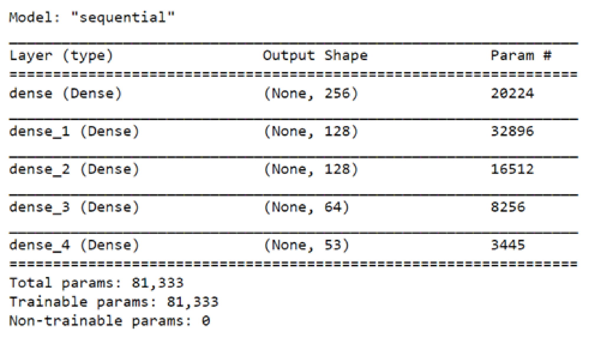
As shown in Figure 3, the ANN model generated more than 81 k parameters during the training phase. The Adam optimization algorithm is used to update the network weights iteratively based on training data. We used the categorical cross-entropy as a loss function, $\Gamma$, which is defined as follows:

$$\Gamma (W,B)=\parallel I-F_{W,B}{\left(I\right)\parallel }^2$$

(8)

3.3.2. RF Structure

RF is a supervised learning algorithm that constructs multiple decision trees. To get an accurate and stable prediction, the final model’s prediction is derived by voting on the class prediction of the individual trees in the forest. Each branch of the tree represents a possible decision, occurrence, or reaction. FR model can be used for both classification and regression problems with a high classification rate.

We built an RF model with a maximum tree depth of 60 and 8 node splits. For an ensembles construct f that has a collection of ensemble classifiers $h_1\left(x\right)$, …, $h_n\left(x\right)$, the ensemble predictor f for a class x is calculated as follows:

$$f\left(x\right)=argmax\sum _{i=1}^{n}I\left(h_i\left(x\right)\right)$$

(9)

where $f\left(x\right)$ is the most frequently predicted class determined by voting between the outputs of $h_1\left(x\right)$, …, $h_n\left(x\right)$ and I is the indicator function that measures the extent to which the average number of votes for the right class exceeds the average vote for any other class. An immense margin value gives more confidence in the classification results.

We used an entropy-based splitting criterion that controls how each tree node splits the data. This has a significant effect on how each decision tree in the forest draws its boundaries.

3.3.3. KNN Structure

We built a KNN model with a K value of 7, which gave us a slightly better classification accuracy. We validated the KNN model using the cross-validation strategy that assesses how our model’s prediction results will generalize to an independent dataset. To recognize an individual class using KNN, we select the K nearest classes to the feature vector by comparing their Euclidean distances. We used the following similarity equation between the two comparable feature vectors ($x_1$, $y_2$):

$$S(x_1,y_2)=1-d(x_1,y_2)$$

(10)

where $d(x_1,y_2)\in [0,1]$ is the Euclidean distance between $x_1$ and $y_2$, and d is calculated as:

$$d(x,y)=\sqrt{\sum _{i=1}^n{(x_i-y_i)}^2}$$

(11)

where $x_i$ and $y_i$ are the Euclidean feature vectors, and n is the n-space dimension of $x_i$ and $y_i$.

4. Implementation

This section presents the implementation details of NetScrapper, including the implementation details of the ML models and the web-based graphical user interface.

4.1. ML Models

Both the RF and ANN models are implemented using Keras development environment [16]. Keras is an open-source neural network library written in Python, which uses TensorFlow [17] as a back-end engine. Keras libraries running on top of TensorFlow make it relatively easy for developers to build and test deep learning models written in Python. The KNN model is implemented using Python programming language.

We set the batch size and number of epochs to be 150 k packet flows and 10 epochs, respectively. The model training was carried out using a server computer equipped with a 4.50 GHz Intel Core™ i7-16MB CPU processor, 16 GB of RAM, and CUDA GPU capability. The training phase took approximately 2 days to run 10 epochs. We took a snapshot of the trained weights every 2 epochs to monitor the progress.

The training error and loss of the ML models are calculated as follows:

$$M=\frac{1}{n}\sum _{i=1}^n{(y_i-x_i)}^2$$

(12)

where M is the mean square error of the model, y is the value calculated by the model, and x is the actual value. M represents the error in class detection.

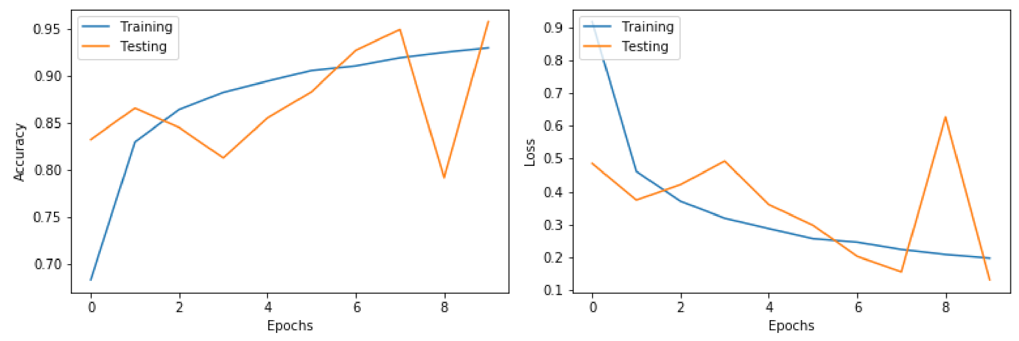
Figure 4 illustrates the calculated training error and loss of the ANN model graphically. As shown in the figure, the mean squared error loss decreases over the ten training epochs, while the accuracy increases consistently. We can see that our ANN model converged after the 8th epoch, which means that our dataset and the fine-tuned parameters were a good fit for the model.

4.2. User Interface

The user interface is developed as a responsive, mobile-first, and user-friendly web application to enhance user experience using the system. We built the web application using Python Flask Framework, HTML5, CSS3, JavaScript, and JSON. All web pages are designed to be device-agnostic that can accommodate visitors using mobile devices, desktops, or televisions to visit the web site.

To run the web application on top of the RF and ANN models, we had to wrap both models, implemented on Keras, as a Representational State Transfer (REST) API using the Flask web framework. REST is a software architectural style used to provide interoperability between heterogeneous computer systems connected via the internet. All communication between Keras and Flask is coordinated through that REST API. When the user captures fresh traffic flow, Flask uses the POST method to send the traffic data from the user browser to Keras via an HTTP header. The Flask service can be accessed by the IP address and port number of the web server without an extension as follows: http://127.0.0.1:5000, accessed on 9 July 2021.

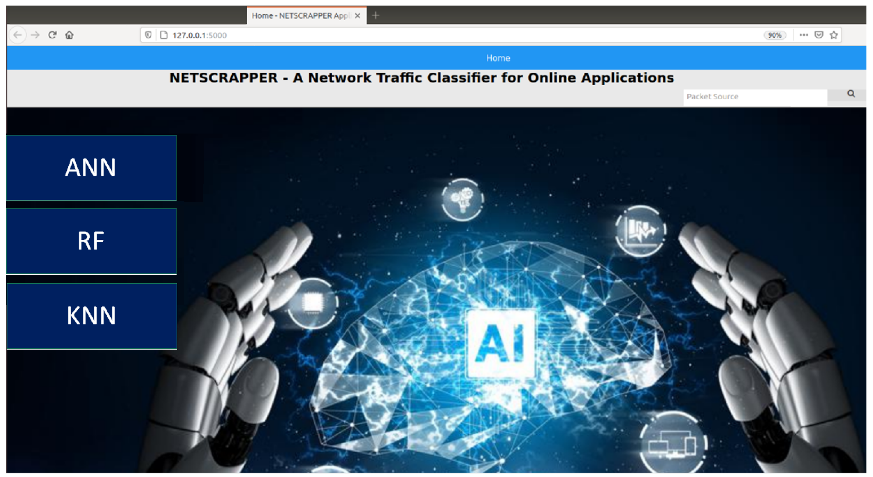
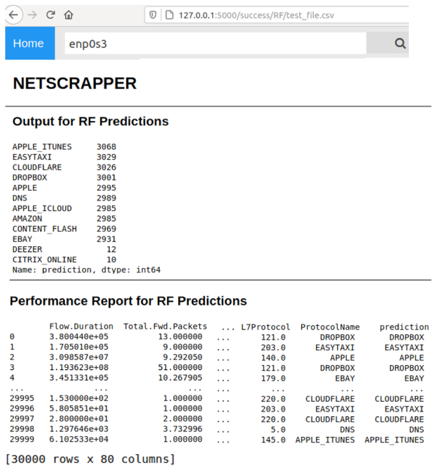
Figure 5 shows a snapshot of the homepage of the web application, which is divided into three modules: ANN, RF, and KNN. Each module allows users to upload a saved snapshot of the traffic flows or capture fresh traffic steam directly from NIC. Figure 6 shows a snapshot of the inference result of the RF model on the web-based GUI. As illustrated in the figure, the web interface displays the flow predictions for all the testing datasets (30 k flow packets × 78 feature attributes), along with the confidence score and prediction time. The additional two columns: ProtocolName and Prediction represent the actual and predicated class names, respectively.

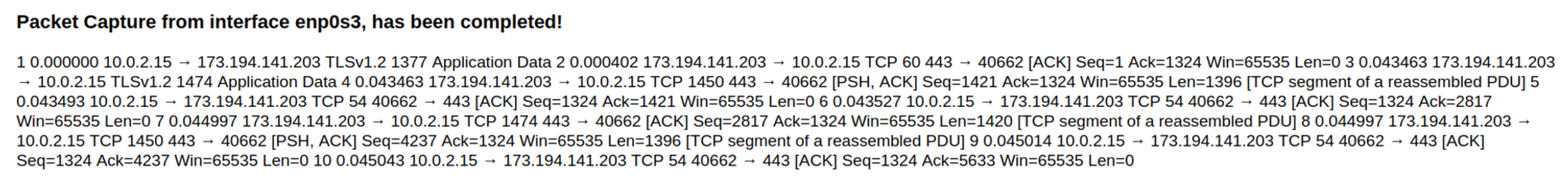
Figure 7 shows a snapshot of the packet sniffing result on the web-based GUI. As shown in the figure, the packet sniffing module can capture and display live network traffic directly from the NIC’s ethernet network peripheral (enp0s3). This raw data is then processed using the CICFlowMeter to extract the required feature vector for the classification phase via the ML pipeline.

5. Experimental Evaluation

We experimentally evaluated our prototype implementation regarding classification accuracy and performance. We installed instrumentation in the web application running on the server to measure the processor time taken to perform various tasks, including packet capturing, traffic flow preprocessing, and prediction processes. Each experiment presented in this section is carried out for ten trials, then we took the average of these trials’ results.

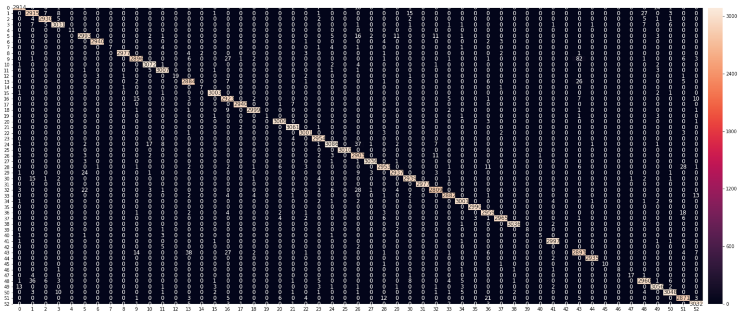
Figure 8 shows the RF model’s confusion matrix, with a heat map for clarity. The matrix gives a detailed analysis of how the model performance changes for different online application classes. The matrix rows represent the actual (true) application classes, and the columns correspond to the predicted application classes. The diagonal cells show the proportion of the correct predictions of our RF model, whereas the off-diagonal cells illustrate the error rate of our model.

The confusion matrix demonstrates that our model, in most cases, can differentiate between the application classes and achieve high levels of prediction accuracy. For the three most common types of online applications, Google, Youtube, and Amazon, the model achieves classification accuracies above 95%, 96%, and 98%, respectively.

We noticed that the application classes in the video streaming category (e.g., Youtube, Netflix, and Twitch) appear easier to identify than the e-commerce (e.g., Amazon and eBay) and social media (e.g., Facebook and Twitter) categories. This seems to make sense as video streaming applications usually use the Secure Reliable Transport (SRT) protocol [18], which is normally carried on UDP connections with low latency and minimal buffering. The SRT protocol relies on establishing a logical channel of communication in which messages flow between the broadcasting server and client, called message stream. Message stream attributes appear more straightforward to identify than those generated by the encrypted communication carried out by e-commerce and social media applications.

As shown in the confusion matrix, our FR model, in some cases, confuses the online applications within the same category (e.g., social media) as they share some common networking attributes such as header and flow descriptors. Note that our ML models can still identify emailing applications (e.g., Gmail and Yahoo) quite well because of their discriminative characteristics compared to the other classes in our dataset. Most notably, although SSL and SSL are considered non-linearly separable classes because of their similar security attributes, our ML models could separate them effectively.

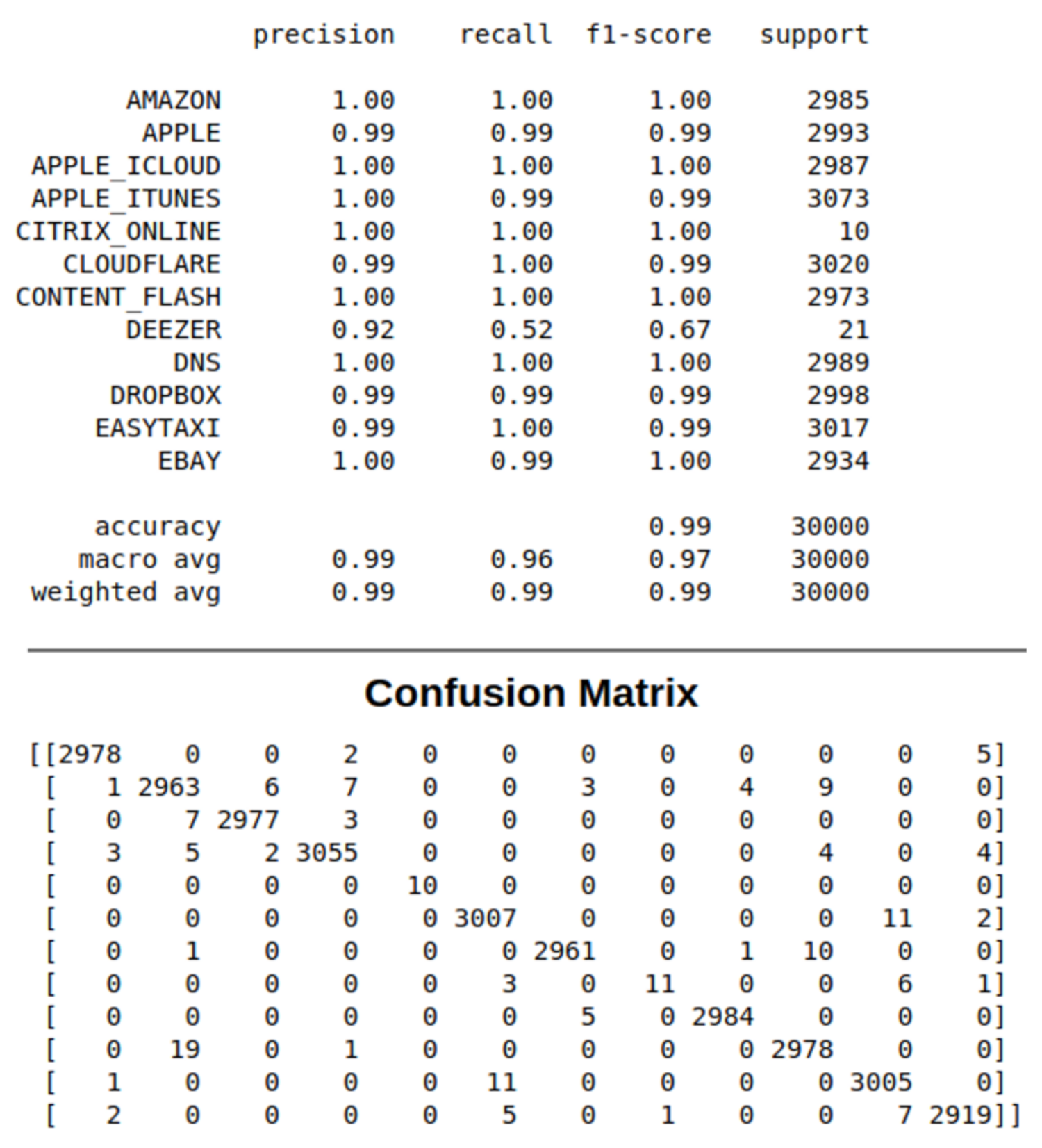
The precision, recall, and F1-score ratios, shown in

Table 3. The precision, recall and F1-score of the RF model.

Class	Precision	Recall	F1-Score	Support
AMAZON	0.95	0.95	0.95	2958
APPLE	0.92	0.91	0.92	2977
APPLE_ICLOUD	0.97	0.99	0.98	2950
APPLE_ITUNES	0.96	0.97	0.96	3062
CITRIX_ONLINE	1.00	1.00	1.00	11
CLOUDFLARE	0.98	0.98	0.98	3046
CONTENT_FLASH	1.00	0.99	0.99	2950
DEEZER	1.00	0.33	0.50	18
DNS	1.00	1.00	1.00	2990
DROPBOX	0.90	0.87	0.89	3028
EASYTAXI	0.97	0.99	0.98	3083
EBAY	0.97	0.98	0.98	3025
EDONKEY	1.00	0.67	0.80	27
FACEBOOK	0.93	0.94	0.94	2932
FTP_CONTROL	0.78	0.78	0.78	9
FTP_DATA	0.99	1.00	0.99	3008
GMAIL	0.84	0.84	0.84	2966
GOOGLE	0.95	0.99	0.97	2948
GOOGLE_MAPS	0.97	0.97	0.97	3014
H323	0.00	0.00	0.00	7
HTTP	1.00	1.00	1.00	3010
HTTP_CONNECT	0.98	1.00	0.99	3064
HTTP_DOWNLOAD	0.99	0.99	0.99	3010
HTTP_PROXY	0.96	0.99	0.98	2958
INSTAGRAM	0.98	0.96	0.97	3164
IP_ICMP	1.00	1.00	1.00	3010
MICROSOFT	0.95	0.97	0.96	2928
MQTT	1.00	1.00	1.00	3042
MSN	0.94	0.93	0.93	3016
MS_ONE_DRIVE	1.00	0.99	0.99	2979
NETFLIX	0.96	0.96	0.96	2967
NTP	1.00	1.00	1.00	2977
OFFICE_365	0.98	0.97	0.98	2879
SKYPE	0.88	0.87	0.88	2913
SPOTIFY	0.98	0.96	0.97	3025
SSH	1.00	1.00	1.00	2990
SSL	0.93	0.95	0.94	2990
SSL_NO_CERT	0.99	0.99	0.99	2988
TEAMVIEWER	1.00	1.00	1.00	3039
TELEGRAM	1.00	0.82	0.90	11
TIMMEU	0.75	0.27	0.40	11
TOR	0.98	0.99	0.98	3002
TWITCH	0.00	0.00	0.00	7
TWITTER	0.84	0.82	0.83	2994
UBUNTUONE	0.99	1.00	1.00	2937
JABBER	0.91	0.83	0.87	12
UPNP	1.00	0.83	0.91	12
WAZE	0.94	0.74	0.83	23
WHATSAPP	0.95	0.90	0.92	3038
WIKIPEDIA	0.97	0.95	0.96	3087
MS_UPDATE	0.95	0.94	0.94	3080
YAHOO	0.91	0.86	0.89	2931
YOUTUBE	0.89	0.96	0.92	3048
Macro Average	0.92	0.88	0.89	126,151
Weighted Average	0.96	0.96	0.96	126,151

, summarize the trade-off between the true-positive rate and the positive predictive value for our RF model using different probability thresholds. Precision represents the positive predictive value of our model, while recall is a measure of how many true positives are identified correctly, and F1-score takes into account the number of false positives and false negatives. The support metric represents the number of samples of the application class in the dataset. As shown in the table, most of the precision vs. recall values tilts towards 1.0, which means that our RF model achieves high accuracy while minimizing the number of false negatives.

The precision ratio describes the performance of our model at predicting the positive class. It is calculated by dividing the number of true positives by the sum of the true positives and false positives, as follows:

$$Precision=\frac{TruePositives}{TruePositives+FalsePositives}$$

(13)

The recall ratio is calculated as the ratio of the number of true positives divided by the sum of the true positives and the false negatives, as follows:

$$Recall=\frac{TruePositives}{TruePositives+FalseNegatives}$$

(14)

F1-score ratio is calculated by a weighted average of both precision and recall, as follows:

$$F1-score=2*\frac{Precision*Recall}{Precision+Recall}$$

(15)

We also observed that our model delivers good results even when flow packets are captures directly from NIC in real time. Figure 9 shows a snapshot of the classification report of the RF model on the web-based GUI. The figure shows that traffic flows from 12 different online applications are captured and predicted using the RF model. Furthermore, our GUI shows the precision, recall, and F1-score ratios of these live streams.

Table 4. The average classification accuracy (%) and prediction time (second) of KNN vs. RF vs. ANN.

	Classification Accuracy			Prediction Time
Class	KNN	RF	ANN	KNN	RF	ANN
AMAZON	97.01	98.79	99.57	283	0.74	0.29
APPLE	86.02	98.62	100	181	0.79	0.28
APPLE_ICLOUD	70.24	99.76	100	190	0.7	0.28
APPLE_ITUNES	97.94	99.43	100	178	0.73	0.28
CITRIX_ONLINE	56.63	100	97.85	92	0.01	0.05
CLOUDFLARE	95.01	98.61	99.97	188	0.66	0.27
FLASH	99.58	99.69	100	251	0.58	0.28
DEEZER	55.5	85.14	99.99	106	0.02	0.05
DNS	99.59	99.82	100	220	0.53	0.3
DROPBOX	91.92	97.35	100	197	0.69	0.39
EASYTAXI	99.3	99.6	100	125	0.75	0.44
EBAY	84.51	99.33	100	163	0.79	0.4
EDONKEY	72.08	90.53	100	202	0.02	0.04
FACEBOOK	98.9	98.96	100	197	0.65	0.4
FTP_CONTROL	49.00	88.00	99.99	144	0.01	0.09
FTP_DATA	99.35	99.9	100	171	0.66	0.34
GMAIL	96.3	97.38	99.92	193	1.01	0.28
GOOGLE	99.46	99.82	99.96	306	0.69	0.29
GOOGLE_MAPS	94.3	99.61	100	159	0.76	0.27
H323	56.54	66.67	99.96	136	0.01	0.04
HTTP	99.24	99.63	100	334	0.65	0.31
HTTP_CONNECT	99.03	99.93	99.89	302	0.67	0.29
HTTP_LOAD	99.79	99.72	100	146	0.68	0.3
HTTP_PROXY	99.45	99.81	99.95	124	0.65	0.33
INSTAGRAM	88.52	98.45	100	145	0.69	0.33
IP_ICMP	99.99	100	100	248	0.48	0.3
MICROSOFT	98.27	98.96	99.56	274	0.68	0.28
MQTT	91.22	99.91	100	168	0.6	0.27
MSN	94.92	98.16	100	162	0.71	0.27
MS_ONE_DRIVE	77.07	99.11	100	149	0.79	0.28
NETFLIX	97.27	99.32	100	141	0.88	0.27
NTP	99.9	100	100	307	0.54	0.27
OFFICE_365	88.34	98.49	100	173	0.76	0.28
SKYPE	94.98	98.25	100	139	0.77	0.28
SPOTIFY	98.75	99.26	100	152	0.75	0.28
SSH	98.29	100	100	238	0.58	0.27
SSL	99.36	98.87	100	236	0.71	0.27
SSL_NO_CERT	99.70	99.61	100	203	0.7	0.29
TEAMVIEWER	98.45	99.94	100	269	0.59	0.27
TELEGRAM	93.06	90.91	98.82	134	0.01	0.04
TIMMEU	79.35	73.53	98.81	104	0.01	0.05
TOR	99.18	99.85	100	193	0.76	0.27
TWITCH	43.60	70.83	99.07	155	0.01	0.04
TWITTER	89.95	96.90	99.67	161	0.79	0.27
UBUNTUONE	99.63	99.97	100	234	0.65	0.33
JABBER	58.43	95.56	99.91	187	0.01	0.06
UPNP	63.77	88.24	99.99	159	0.01	0.05
WAZE	81.00	92.41	99.91	146	0.02	0.04
WHATSAPP	97.48	98.24	100	158	0.78	0.28
WIKIPEDIA	87.11	98.85	100	170	0.82	0.28
WIN_UPDATE	98.85	99.19	100	250	0.66	0.28
YAHOO	99.67	97.54	100	174	0.76	0.27
YOUTUBE	96.82	99.43	99.81	129	0.77	0.27
Mean	88.86	96.33	99.86	187.66	0.56	0.25

compares the KNN, RF, and ANN models in terms of classification accuracy and prediction time across the 53 classes. For instance, the ANN model achieved an overall average classification accuracy of 99.86%. The average prediction time of the model was measured to be 0.25 s. This is evident that administrators can detect any security vulnerability in their networks using a handy web-based GUI in a quarter of a second. Furthermore, we noted that the prediction accuracy of many classes (e.g., Netflix, Dropbox, and WhatsApp) was 100%. This shows that our model is robust and can operate in real-time inference in real-world network settings with high accuracy.

Compared to ANN and RF, KNN is considered a significantly slower model in the case of having a large dataset because it needs to scan all the training databases each time a prediction is required; thus, it cannot generalize over the dataset in advance. That is why we believe that the KNN model is not adequate to be used for real-time inference. In contrast, on average, the ANN model requires around 250 ms only to detect a security thread in a traffic flow. To put these numbers in some context, consider a firewall service installed in a gateway router; our ANN model can inspect around four applications’ flow streams per second, which would have a negligible latency overhead over the network stream.

6. Conclusions and Future Work

This paper presented the design and implementation of NetScrapper, an AI-enabled network classifier for real-time flow streams. The developed prototype showed that NetScrapper could be deployed on networking devices at the edge with high prediction accuracy and low response time. It is expected that NetScrapper would make a better opportunity for network administrators to monitor their network performance and detect any suspicious traffic that could harm the network components and legitimate users. Unlike most of the existing ML-based classifiers, NetScrapper can automatically extract the feature attributes of the online traffic flow without human intervention, which undoubtedly makes it a highly desirable traffic classification approach, especially for mobile services encrypted traffic.

The system implementation compared three ML models, namely ANN, RF, and KNN, in terms of classification accuracy and performance. To increase the system usability, we developed a user-friendly interface on top of these models to allow users to interact with the system conveniently. We carried out several sets of experiments for evaluating the performance and classification accuracy of our system, paying particular attention to the prediction time. Our ANN model could most notably inspect four applications’ flow streams per second, which proves that NetScrapper is suitable for real-time inference at the edge with offline generated ML models.

We expect that this research would increase the open-source knowledge base in the area of traffic analysis and machine learning on the network edge by publishing the source code and dataset to the public domain. Both the source code and dataset are available online: https://github.com/ahmed-pvamu/NetScrapper (accessed on 9 July 2021).

In on-going work, we are looking into opportunities for generalizing our approach to be deployed locally at all types of network devices at the edge, where administrators can use to monitor their network from any point in the network topology. This would give them a richer picture of their network performance and reduce the time associated with detecting security threats and intrusions.

We also plan to train a multi-level classification algorithm to enable NetScrapper to identify traffic flows from unknown application sources. If an unknown packet is detected, the system will automatically add it to our training database of unknown classes. This technique would also use an unsupervised clustering algorithm to label the unknown packets as discrete classes. We are also working on using the Actor model of concurrency [19], leveraging multi-threaded computation for massive live traffic streams. It will be useful for supporting the sensing needs of a wide range of researches [20,21,22,23,24,25,26,27,28,29,30] and applications [31,32,33,34,35,36,37,38,39,40]. Finally, experiments with more massive datasets are needed to study the robustness of our system at a large scale, and improve the prediction accuracy of the less performing application classes.