The required background notions on Rough Sets, Feature Selection and QuickReduct are outlined hereafter, followed by the detailed description of the proposed AdaptiveQuickReduct algorithm and its limitations.
2.1. QuickReduct for Feature Selection
Let
U be the universe of discourse and
A be a finite set of attributes; let
be an information system: an
equivalence relation in
I is the set of objects belonging to
U that are not discernible by attributes in
P, defined as follows:
It can represent any
, where each attribute
A has values in
, such that
,
.
Every equivalence relation defines a partition set of
U, called
, that splits
U in equivalence classes called
[
7]. According to [
8], equivalence classes correspond to information granules and can be used to approximate any subset
through a pair: its
lower approximation (Equation (
7)) and its upper approximation (Equation (
8)).
The
positive region—given two equivalence relations called
C and
D over
U—is defined as:
and represents the union of the lower approximations of all the equivalence classes defined by
. From the definition of the positive region it is possible to derive the
degree of dependency of a set of attributes
D on a set of attributes
C, called
:
A reduct
is the subset of minimal cardinality of the set of conditional attribute
C such that its degree of dependency remains unchanged:
where
is the set of decision features and
is the set of conditional attributes.
A reduct is minimal, meaning that no attribute can be removed from the reduct itself without lowering its dependency degree with the full set of conditional attributes. Most of the feature selection algorithms used in Rough Set theory are based on the definition of reduct and on the efficient construction of the optimal reduct [
9,
10,
11,
12].
The QuickReduct [
13] (please see Algorithm 1, called QR from now on) builds the reduct concatenating the attributes with the greatest increase in the dependency degree, up to its maximum in the considered dataset. Being the exploration of all possible feature combinations computationally unfeasible, QR uses a greedy choice: it adds one at a time to the empty set the attributes resulting in the greatest increase in the Rough Set dependency degree until no other attribute can be added. In this way, it is not guaranteed to find the optimal minimum number of features, however it derives a subset sufficiently close to optimal in a reasonable time, resulting in general a good compromise between time and performance to reduce the dataset dimensionality in many real world scenarios [
14].
| Algorithm 1 QuickReduct |
- 1:
procedureQuickreduct(C,D)
- 2:
- 3:
- 4:
- 5:
repeat - 6:
- 7:
for do - 8:
if then - 9:
- 10:
- 11:
until - 12:
return R
|
2.2. Adaptive QuickReduct
In order to exploit the idea underlying QuickReduct in an evolving scenario, it is necessary both to detect feature drifts and to change the selected features accordingly. The ideal algorithm should not only add new features that increase the dependency degree of the selected reduct as new data are processed, but also remove the previously selected features whose contribution is no longer relevant.
A typical approach to analyze data streams consists in choosing a windowing model and processing data in each windows, with a moderate overlap between consecutive windows.
Assuming that a reduct is available at time in the window , the goal is to evaluate whether the features remain those with the highest dependency degree with respect to at time and in the window , i.e., if ) or if there is a new better subset .
Two steps are needed: first the removal of the redundant features in
and then the addition of new features that increase the dependency degree for
. The proposed algorithm, called AdaptiveQuickReduct (AQR from now on) implements exactly this strategy: given a reduct
calculated in the time window
, the first step iteratively removes all the features
such that
. The output of this step is a new reduct
to be eventually expanded with new features. In particular, let
be the set of features removed from
, the second step consists in trying to add new features
to
following the QuickReduct schema. Pseudocode for AQR is reported in Algorithm 2, while Algorithm 3 reports a driver program that acts as a detector and shows how AQR can be called with a sliding window, in which parameter
W represents the window size (batch) that moves forward by
O instances at each iteration.
| Algorithm 2 AdaptiveQuickReduct |
- 1:
procedureAdaptiveQuickreduct(C,D,R)
- 2:
- 3:
- 4:
- 5:
repeat - 6:
- 7:
for do - 8:
if then - 9:
- 10:
- 11:
- 12:
until - 13:
- 14:
repeat - 15:
- 16:
for do - 17:
if then - 18:
- 19:
- 20:
until - 21:
return R
|
| Algorithm 3 FeatureDriftDetection |
- 1:
procedureFeatureDriftDetection(,,W,O) - 2:
- 3:
- 4:
- 5:
- 6:
- 7:
- 8:
- 9:
repeat - 10:
- 11:
remove O oldest instances from C - 12:
remove O oldest instances from D - 13:
add O new instances to C - 14:
add O new instances to D - 15:
until end of stream
|
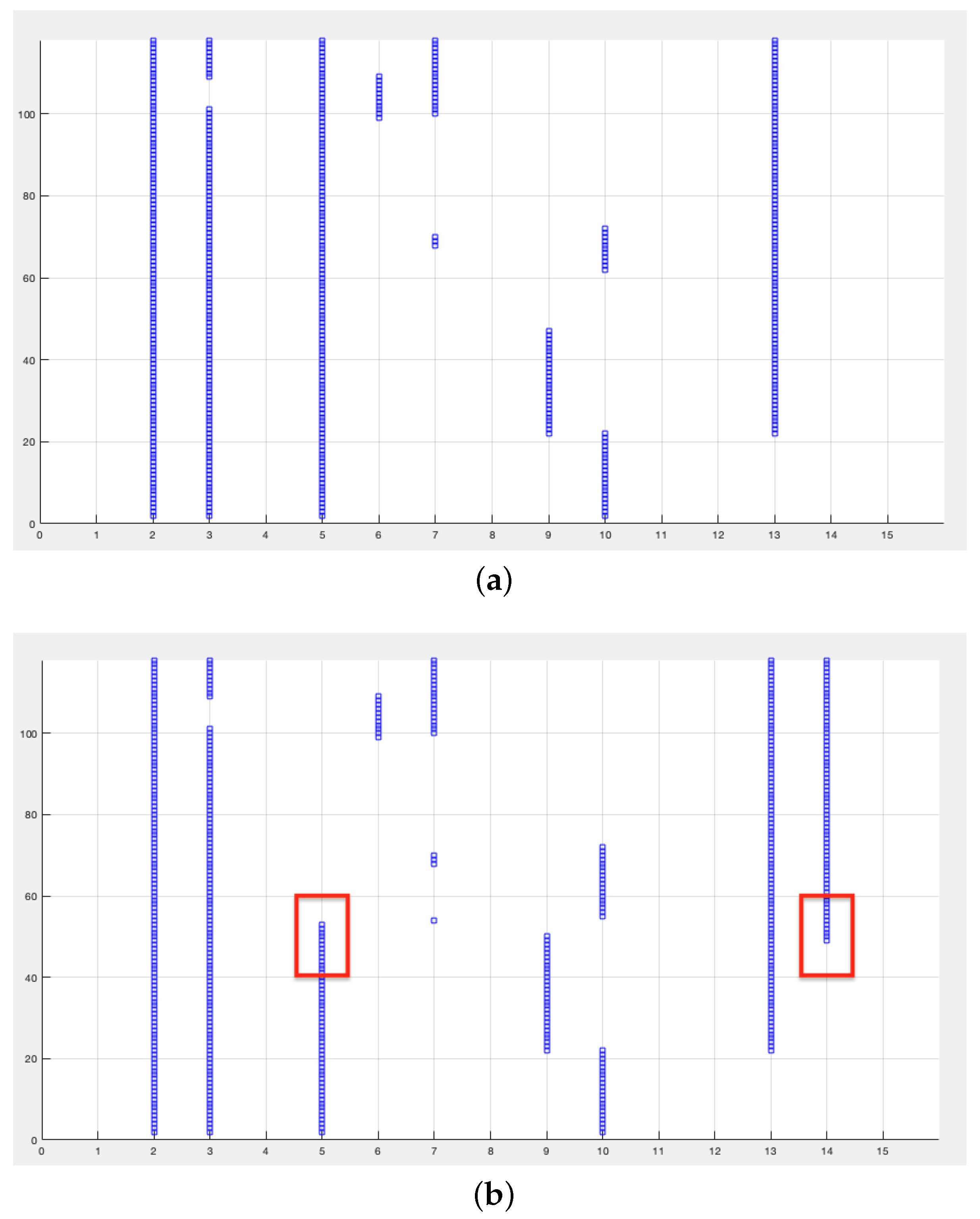
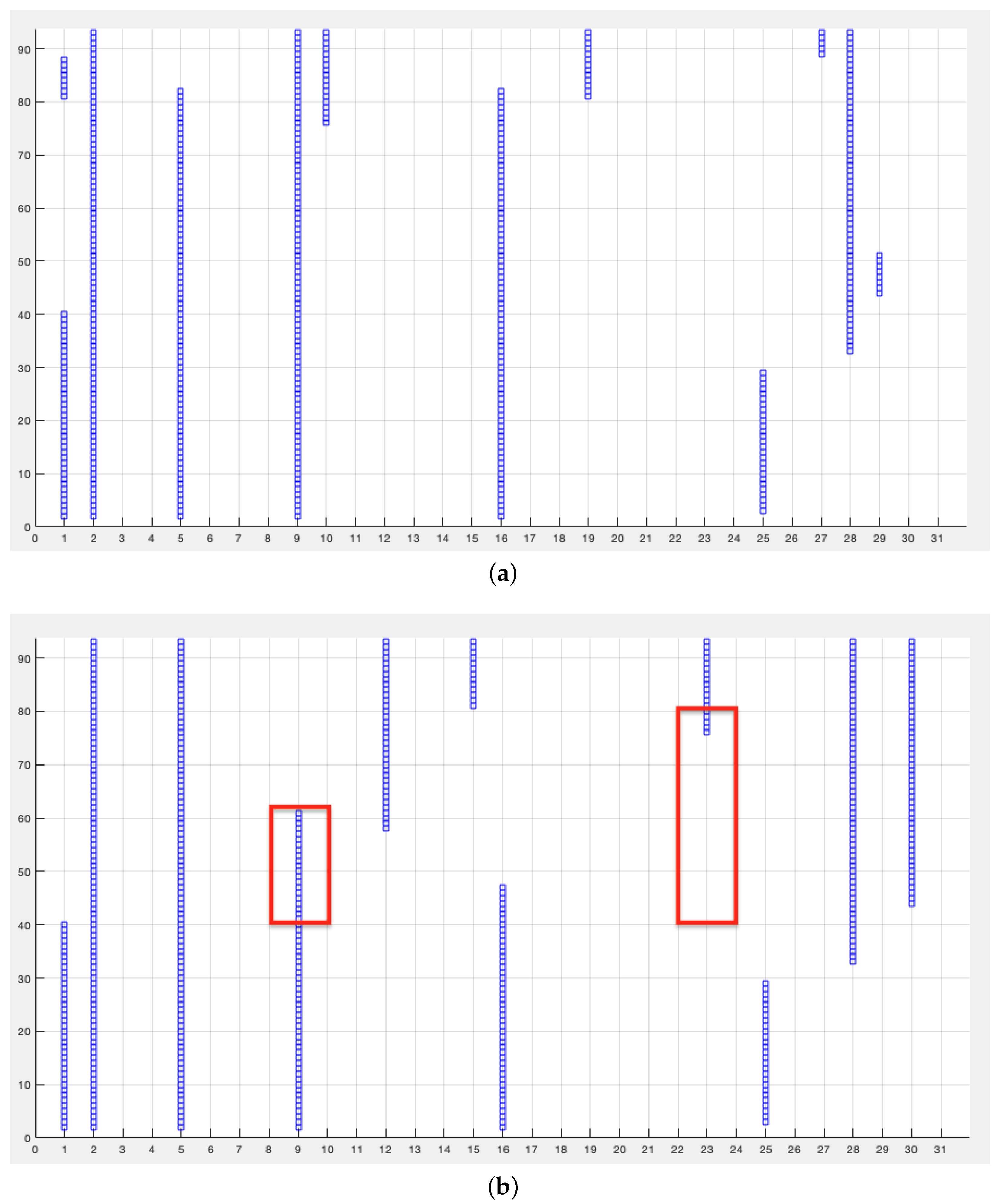
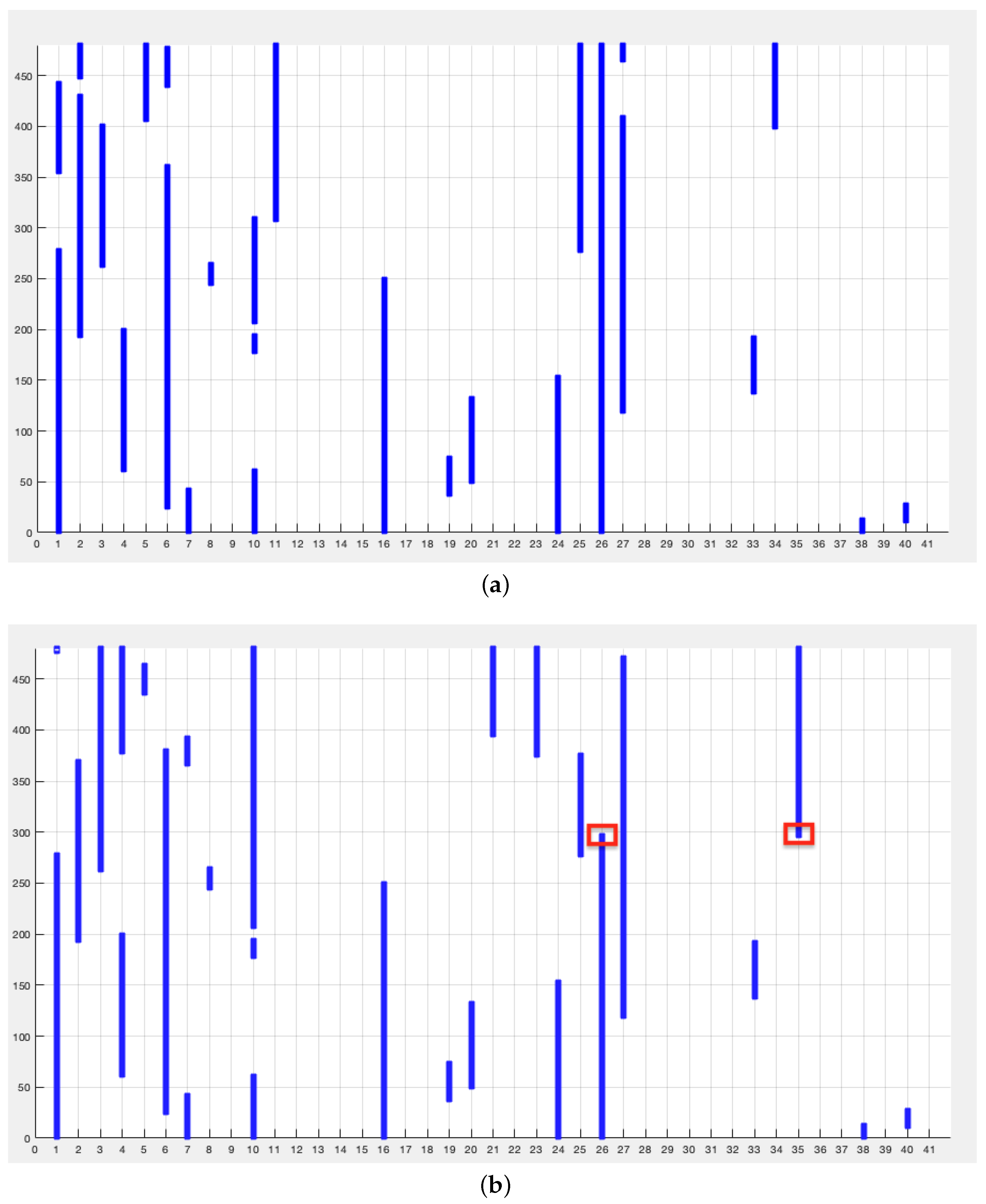
Although it is possible to detect gradual or incremental drift considering a thresholding function T, the definition of a continuous relevance score would be required, which is not explicitly available in QR as it does not give a weight to the features to be selected. On the contrary, the sudden change that occurs at a precise moment—feature shift—is easily detectable through a qualitative analysis of the output.
As stated in
Section 2.1, a minimal reduct is a subset of the dataset conditional features that has equal rough dependency degree as the full set of features and such that no strict subset of this reduct exists that has a greater dependency degree. It must be stressed that the variation in dependency degree given by the addition or deletion of a single feature, even though effective, does not guarantee to predict the optimal reduct, but in general a super-reduct (a subsets that has maximal dependency but not the smallest cardinality). This limitation is in common with QR and it is due to their greedy nature, consequence of the unfeasibility of exhaustive search for the optimal reduct [
15]. Nonetheless, as proven by the successful application of QR in countless domains, even the sub–optimal reduct is a sufficiently good approximation in most real world application (see for example [
16]).
Other approaches to Feature Drift detection are Dynamic Feature Weighting (DRW, see [
17]), where the weight of each feature is increased or diminished according to its relevance obtained through entropy or symmetrical uncertainty on sliding windows; or methods based on Hoeffding Trees (see [
18]), that is Decision Trees that use the Hoeffding bound to compute an arbitrarily close to optimal Decision Trees on the base of a limited amount of streaming data (see [
19,
20,
21]). Even ensembles have been proposed to extend methods based on Hoeffding Trees, at the cost of an higher computational burden [
22]. To the best of our knowledge, none of these exploits fuzziness or roughness in detecting drifts.


