Abstract
K-Means Clustering is a popular technique in data analysis and data mining. To remedy the defects of relying on the initialization and converging towards the local minimum in the K-Means Clustering (KMC) algorithm, a chaotic adaptive artificial bee colony algorithm (CAABC) clustering algorithm is presented to optimally partition objects into K clusters in this study. This algorithm adopts the max–min distance product method for initialization. In addition, a new fitness function is adapted to the KMC algorithm. This paper also reports that the iteration abides by the adaptive search strategy, and Fuch chaotic disturbance is added to avoid converging on local optimum. The step length decreases linearly during the iteration. In order to overcome the shortcomings of the classic ABC algorithm, the simulated annealing criterion is introduced to the CAABC. Finally, the confluent algorithm is compared with other stochastic heuristic algorithms on the 20 standard test functions and 11 datasets. The results demonstrate that improvements in CAABA-K-means have an advantage on speed and accuracy of convergence over some conventional algorithms for solving clustering problems.
1. Introduction
Clustering procedure [1,2,3] is a process that divides a set of objects into clusters according to the predefined criteria such that objects in the same cluster are more parallel to each other than other objects in different clusters. Clustering is often used in solving a part of complicated tasks in pattern recognition [4], image analysis [5], and other fields on data processing [6]. An excellent clustering algorithm still has a higher interference-free capability and lower time complexity than traditional algorithm when processing large amounts of data. The clustering algorithms can be subdivided into two categories: hierarchical clustering and partitional clustering. The hierarchical clustering algorithm divides the pattern into fewer structures continuously, and it is usually described by the tree structure. Partition clustering is the division of a set of objects into K non-intersecting subsets with high internal similarity. The center-based clustering algorithms are the most popular partitional clustering methods.
K-means is simple and efficient, in which case it becomes one of the most popular center-based cluster methods [3]. However, relying on the initialization of K states and convergence towards the local minimum are significant shortcomings of K-means classification. In order to overcome these problems, many other methodologies have been applied to algorithm. A clustering algorithm which based on genetic algorithm was proposed by Mualik and Bandyopadhyay, and its effectiveness is proved on real-life datasets. Simulated Annealing (SA) approach is proposed to solve the clustering puzzle by Selim and Al-Sultan (1991). Beyond that, many heuristic algorithms like Particle Swarm Optimization (PSO) [7], Differential Evolution (DE), and ABC, have also been successively adapted in the clustering algorithm optimization improvements.
ABC is a swarm intelligence algorithm that is derived from the honeybee colony’s gathering behavior. After Turkish scholars Karabogac Denis raised this problem in 2005 [8,9], it was widely applied to solve function optimization problems, for the advantages of less parameters, simpler structure, and being easier to implement [10]. Compared with PSO and Genetic Algorithm (GA), ABC’s advantage is proved further in Section 4. Similar to other swarm intelligence algorithms, the performance of optimized ABC mainly depends on its search strategy. Due to the randomness of the search mechanism, the algorithm is easy to get stuck at local optimal value and has slow convergence speed. ABC has been optimized gradually after the proposal, and it has been extended to various fields. Inspired by PS0 algorithm, the global optimal solution is used to guide the search formula (GABC) in [11]. Inspired by the DE algorithm, another new improved algorithm MABC was proposed. In [10], comparing with the original ABC algorithm, the MABC modifies the employed bee stage and onlooker bee stage, which improves the efficiency. The proposed algorithm is then applied to solve a loudspeaker design problem using FEM. The CGABC based on the crossover is proposed in [12]. The Crossover operator of genetic algorithm is introduced into the Global optimized Artificial Bee Colony algorithm. Crossover is the transfer of good genes from the parent of a population to its offspring. The brand new ABC_elite is proposed in [13]. To better balance the tradeoff between exploration and exploitation, it proposes a depth-first search (DFS) framework. The article introduces two novel solution search equations which incorporates the information of elite solutions and can be applied to the employed bee phase. Furthermore, many studies increase search efficiency by changing the greedy search mechanism. Sharma T K [14] changes the search path of scout bee. Two new mechanisms for the movements of scout bees are proposed. In the first method, the scout bee follows a non-linear interpolated path while in the second one, scout bee follows Gaussian movement. Yang, Weifeng Gao [15,16] improves the greedy search and adapts to more optimization problems using introduced adaptive methods. In addition, to enhance the global convergence, when producing the initial population and scout bees, both chaotic systems and opposition-based learning method are employed. Xiang W L [8] proposes a depse-first search framework. Gao W [17] increases information sharing among individuals through improvement. In addition, many scholars [18,19] choose to combine the ABC algorithm with other familiar algorithms for optimization. Each bee should select whether adopts greedy strategy or not based on its fitness value on each generation. A great progress in solving complex numerical optimization problems has achieved in [19,20]. With the continuous improvement and optimization, ABC has been applied in more fields, such as workshop scheduling [21,22,23,24,25] software aging prediction [26], machine learning [27], multi-objective optimization [28], dynamic optimization [29,30] and so on.
ABC has unique advantages for data optimization problems. In this work, the improved ABC is extended to clustering procedures. Crossover operation and adaptive threshold are integrated to improved ABC algorithm. The simulated annealing technique and Fuch chaotic perturbation operation are drawn into the algorithm. Furthermore, the initialization equation and the fitness function are reformed according to the shortcomings of the K-means. The CAABA-K-means has been proved to be superior on speed and accuracy of convergence over some conventional algorithms for solving clustering problems.
The remainder of this work is distributed as follows: Section 2 discusses the ABC algorithm and clustering analysis problems. The chaotic adaptive ABC (CABC) algorithm adapted for solving K-means clustering problems is introduced in Section 3. Section 4 shows that our method outperforms some other methods by showing experimental studies. Section 5 is the conclusion, which summarizes our proposed method.
2. Relative Work
2.1. Artificial Bee Colony Algorithm
ABC is a swarm intelligence algorithm, which imitates the division of labor and the search mode of bees to find the maximum amount of nectar [8]. In the classic ABC algorithm, the artificial bee colony is divided into three categories according to their behaviors: employed bee, onlooker bee, and scout bee. In the beginning, the number of employed bees equals to onlooker bees, and the third kind of bees appear gradually. The employed bee uses information about the initial honey source to find new honey source and shares the information with the onlooker bee. The onlooker bee waits in the hive and chooses a better source according to the greedy selection mechanism. However, if the honey source information has not been updated for a long time, the corresponding employed bee will be transformed into a scout bee. The task of scout bee is to search for the honey source randomly around the hive and find a new valuable honey source eventually. Self-organization, self-adaption, social division, and collaboration are significant features of the entire colony. ABC simulates the foraging behavior as the process of searching for the optimal solution, defines the adaptability to the environment of individuals as the objective function of the problem to be solved, and takes the greedy selection method as the basis for eliminating the different solution. This process is iterated until the optimal solution is reached and the entire function gradually converges. The steps can be described specifically as follows.
2.1.1. Initialization Stage
In ABC algorithm, the fitness value represents the quality of nectar sources and candidates solution corresponding to food sources. It is assumed that the population size is . The initial solution is obtained through Equation (1).
where is the -th component of the -th vector. , . and are the upper bound and lower bound of the -th component, and is a random number from 0 to 1. The algorithm executes global searching randomly for food sources and derives the revenue value.
2.1.2. Employed Bee Stage
After initialization, the ABC algorithm starts the stage of employed bees. Employed bees search randomly around the current region according to Equation (2) and shares the information with the onlookers; thus, a new set of honey sources, , is generated
where , . In addition, is the index, which is chosen randomly. In addition, is a necessary requirement to reduce duplication of effort. If the fitness value of a new source is ameliorated, the source will be superseded by the new one.
2.1.3. The Probability of Selecting the New Food Source
The fitness value is calculated by Equation (3), which is an evaluation criteria of nectar source quality.
where . denotes the fitness value of . The larger value means the higher quality of honey source. In addition, is the value of the -th nectar source′s objective function.
When the fitness values are calculated, they are applied to calculate the probability of selecting the -th honey source , which can be used as a basis for onlooker bees to select honey sources.
where denotes the fitness value of the .
2.1.4. Scout Bee Stage
If the search steps reach a certain threshold, but no better position is found, the position of this employed bee is re-initialized randomly according to Equation (1).
Each food source is verified by employed bees and/or onlooker bees for its potential inclusion as a candidate position. The ABC algorithm utilizes employed bees, onlooker bees and scout bees to iteratively search the solution space until reach the maximum number of iterations. If a food source is not improved further through limit trials, it is deemed as an exhausted source and abandoned. Under different conditions, the three kinds of bees transform into each other and the result gradually approaches the optimal solution. The transformation diagram is as Figure 1.
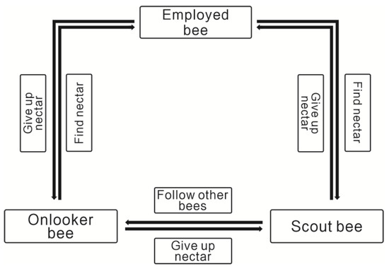
Figure 1.
Structure Diagram of Artificial Bee colony Algorithm.
2.2. K-MEANS Cluster Algorithm
Clustering methods are suitable for finding internally homogeneous groups in data. The K-means algorithm is one of the oldest clustering techniques [1], which is constructed based on the iterative hill-climbing process. The main idea is to gather the original data into K clusters according to similar attributes. The main processing procedure is as follows. Firstly, K samples are randomly selected from the original data, and each sample is taken as the center of K clusters. Then the distance between the K center samples and the remained samples is separately calculated. According to the calculation, each sample is classified into the nearest cluster. The iterative process is repeated until the cluster no longer changes. Therefore, the traditional K-means clustering is expressed as follows.
is the original data sample, where is -dimensional vectors. is the cluster sets, where is the number of clusters.
K-means criterion function is expressed as follows:
where represents the distance between data and its clustering center , and represents sum of its internal distances.
3. Chaotic Adaptive Artificial Bee Colony (CAABC) for Clustering
During the iterative optimization process of the classic ABC algorithm, both employed bee and onlooker bee follow a completely random search strategy. As a result, the ABC algorithm has strong global search capabilities. However, the algorithm selects the honey source blindly at the stage of the employed bee. Only the random number , between –1 and 1], can be used to control the search region of the neighborhoods, and the search direction of onlooker bee is guided by the information of honey source from employed bee. In the entire iteration process of the algorithm, the blindness and randomness make the algorithm more complex and sacrifice the accuracy of algorithm results. For balancing the exploration and exploitation performance, ABC has been optimized from different perspectives. To improve the convergence speed, GABC combines the ABC with PSO algorithm and the global optimal solution is referred to change the random neighborhood searching of classic ABC, which enhances the exploitation performance of algorithm. However, simply adding the global optimal solution not only enhances the convergence speed but also increases the risk of premature convergence. Therefore, inspired by GABC, the information carried by ordinary individuals in this paper is effectively utilized and the search space is adaptively adjusted to avoid premature convergence. In order to overcome the disadvantages of K-means clustering algorithm, such as over dependence on the initial clustering center, easily falling into local optimum, and the premature and slow convergence of the artificial bee colony algorithm due to the limitations of search strategies, a hybrid clustering method combining the improved artificial bee colony algorithm and K-means algorithm is proposed which makes full use of the characteristics of the improved artificial bee colony algorithm and K-means algorithm.
3.1. MAX–MIN Distance Product Algorithm
Initialization affects the global convergence and the performance of the algorithm, so it is particularly important in the evolutionary algorithm. K-means clustering algorithm has high sensitivity to the initial stage. Based on [31,32], we propose a max–min distance product algorithm for initialization. The initialization process not only reduces the randomness of colony initialization but also reduces the sensitivity of Kmeans clustering to initial points. In [33], the max–min distance means is used to search the optimal initial clustering center, in which case convergence speed and accuracy of the algorithm have been significantly improved. However, it may lead to clustering conflict when the initial clustering center is excessive dense. The maximum distance method proposed in [34] reduces the number of iterations effectively, but there would be the problem of initial point deviation. It is possible that the product of two distances is the same, but the density of the points is quite different.
To improve the efficiency, we propose a max–min distance product algorithm. We can get from according to Equation (6). represents the product of the maximum and minimum values in .
where points are randomly selected as the initial cluster centers from the original data set. Meanwhile, is a data set used to store the distance between other points in the data set among cluster centers. is an array that stores the product of elements in . is the product of the maximum center distance and the minimum center distance. The points that corresponding to the are selected as cluster centers instead of initial points. The distribution of current initial points can be dispersed by the max–min distance product. Moreover, it can avoid the situation that two distance products are equal, but the point density of their regions is quite varied, and magnify the difference between points. The enhanced selection method is better.
3.2. New Fitness Function
Fitness function is the crux of population evolution, which determines the solution quality directly. It is the key factor which affects the stability and convergence of the algorithm. Based on the characteristics of the iteration of ABC and the basic idea of the K-means algorithm, a new fitness function is adopted in this work:
where represents the number of samples in the -th cluster.
denotes the sum of the distance between the sample points among the centers. The new fitness value can give rise to equilibrate the influence of the numbers and distance of samples. The phenomenon of inaccurate judgment caused by the same value of or is avoided, which improves the adaptability of the function and makes the iterative process more accurate.
3.3. New Position Update Rules
3.3.1. Arregate-Dispeise Algorithm
To improve convergence speed and accuracy, aggregate-disperse algorithm is introduced here. On the basis of the simplex method, we propose an “aggregate-disperse operation” as a guiding strategy for the iteration. According to the relationship among the global optimal solution, elite solution and ordinary individual, the search range and step length change adaptively.
- The Simplex Method
The simplex method is a traditional optimization method which uses the iterative transformation of the vertex of the geometric graph to approach the optimal value gradually. Take a dual function as example. Take three points , which are not collinear, as the vertices to form a triangle. Calculate the function value and compare them to each other. Calculate the function value and compare them to each other.
- (1)
- means is the worst solution, and is the best one. The algorithm should search in the opposite direction to find the minimum. is the midpoint of , is on the extension line of , and is called the reflection point of with respect to :where is the reflection coefficient, which equals 1 as usual. The geometric relationship is shown in Figure 2:
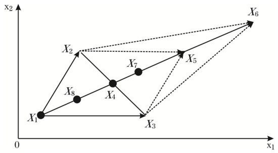 Figure 2. The Simplex Method.
 - (2)
- denotes that that direction of searching is correct, the algorithm should keep going in this direction. Let . If , is replaced by to form a new simplex, or is dropped.
- (3)
- means that the searching is going in the right direction, but doesn’t need to expand.
- (4)
- demonstrates that has gone too far to need to be retracted.
- (5)
- If , need to be retracted toward .
- Aggregate and Disperse Operator
The purpose of the aggregate operation is to provide guidance for the population gathering in a potential direction during the iteration. With this operation, the algorithm can increase the convergence speed in the initial stage and strengthen the local search ability in the later stage. , , are three given solutions, the worst individual is moved toward the others. In order to accelerate the convergence speed, the elitist solution and the global optimal solution are used to guide the search process.
The parameter setting is [31] to ensure that the new solution maintains convergence while moving toward a better direction generally. can be considered as the punishment parameter for the poor individual, and -α is the encouragement parameter.
denotes that the better solution is not found, so the influence of the original strategy should be moderately weakened.
denotes that the original strategy should be strengthen.
The parameters are transformed to form a convex combination to avoid negative weight in the later stage.
The simplex method and ABC are fused in the two-dimensional coordinate space in Figure 3:
where . The vectors OA, OB, and OC represent the global optimal solution, elite solution, and ordinary individual respectively. If , according to convex combination analysis, the point lies on the line segment , and ends up in the triangle . When the searching area is extended to n-dimensional space, the point will fall into an area with the line segment as the median line, which is the potential space limited by elite solutions and globally optimal solutions. Finally, multiple planes intersect at the global optimum. The results converge to the globally optimal solution with high probability.
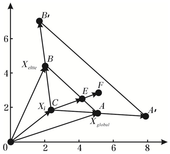
Figure 3.
Aggregate Operation.
However, if the three solutions are collinear, it will be trapped in the local optimum because the search space is too narrow. Therefore, the disperse operation is used to expand the search space.
The vectors are random numbers between 0 and 1. After the dispersion operation, the search area is extended to triangle area . In multidimensional space, multiple planes intersect at the global optimum with high probability eventually. Figure 4. demonstrates the disperse operation in the two-dimensional plane.
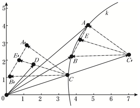
Figure 4.
Disperse Operation.
3.3.2. Adaptive Adjustment
In the iterative process of ABC algorithm, the neighborhood search range is controlled by a random parameter, and the neighborhood search is performed randomly and aimlessly. The effectiveness of the algorithm is influenced by the blindness and randomness visibly. In order to remedy the defects, an adaptive parameter is used to adjust the algorithm’s search step length. Furthermore, in order to have stronger adaptive performance, we replace the fixed-size parameter with an alterable one, , during the iteration.
where . and are the number of current iteration and the maximum iteration severally. As is shown in Equation (13), the step length factor decreases and adjusts adaptively with the iteration process. In the initial time, the global searching is executed efficiently with a large step length, and the step length is variable in the later process to achieve a detailed local search.
3.3.3. Genetic Crossover
The randomness of the searching method limits the optimization ability and affect the convergent rate of canonical ABC. To balance the performance of the algorithm, the crossover operation is carried out to intersect with the global optimal solution based on unbiased adaptive optimization. The main goal of the GA algorithm is for reference, and the diversity of the population and overall optimization ability are further increased by crossing with the excellent parent generation. Crossover operations are performed to find more valuable individuals in the searchable space. The larger the size of the intersection, the more combinations of the allogeneic genes are exchanged, and the wider the searchable range is. However, with the expanding of the size of the intersection, the increase of searchable scope shrinking. The larger the scope of the crossover operation means the smaller the probability that any individual in the space can be searched. Therefore, the probability of excellent vertices being searched will affected by the scope of intersection. CR is the local search coefficient, that is used to control the activity of individuals during the local search. The smaller the value means the more active of individual’s behavior.
The improved algorithm in this paper has as good local search ability because of the ergodicity of chaotic search. Combined with the characteristics of gene crossover and the ergodicity of the chaotic disturbance, we conduct a comparative test for different CR values from 0 to 1, and finally concludes that the algorithm can achieve better performance when CR = 0.6.
Combining the improvements above, we can get a new position updating formula, the calculation process is shown as Equation (14).
If the location of three solutions is on the same line, the position updating criterion is changed to Equation (15) on the base of disperse operation:
In the iteration, the cross factor , represents the global optimal solution, is the ordinary individual selected from randomly, and is the elitist solution. After sorting the solution, is selected from the top solutions randomly, where is the population number, and .
In order to verify the effectiveness of the improved method in this part, the improved ABC algorithm whose position updating according to the “aggregate-disperse operation” and cross operation is temporarily named CAABC-2. As the components of CAABC, its effectiveness will be proved in the fourth part.
3.4. New Chaotic Disturbance
Chaos is a unique movement pattern of a nonlinear system with particular features of sensitivity to the initial value, randomness, and ergodicity. Chaotic search is generated by iterating chaos sequence through a certain particular format and extending the numerical range of the chaos variables to the value range of the optimization variables through the form of the carrier wave. Fuch chaos [32], as a new type of discrete mapping, has unique advantages over logistic chaotic mapping, with more optimized chaotic performance and fewer iterations. It is proved that the chaotic map has no rational number fixed point, then the mapping relational formula is used to establish a chaotic model that is used to solve the Lyapunov exponent, and the sensitivity of chaotic maps to initial values is investigated under large variation and small variation on initial starting points. The chaotic map is then used to establish chaotic generator to replace the finite-collapse map, and to improve the dynamic performance of chaotic optimization. The method improves the search efficiency by continuously reducing the searching space of variables and enhancing search precision. It is more ergodic and does not fall into local optimum with incorrect initial value setting. The expression is:
Thus, iteration sequence is obtained. In the formula, ;
The Lyapunov exponent of Fuch chaos is solved in [32], and the results shows that Fuch chaos has a stronger chaotic property and a more homogeneous ergodic property than Logistic chaos and Tent chaos.
In this work, the adaptive value of the function is computed based on a novel function and the chaotic disturbance is increased to 15% of individuals with poor performance and the elite solution to update the historical optimal adaptive value. If the new solution is superior, the new position will be used to replace the original one. The chaotic algorithm can effectively avoid converging on local optimum and gain higher precision.
To verify the effectiveness of the Fuch chaos in the CAABC, on the basis of CAABC-2, chaotic disturbance is added. It is named CAABC-1 temporarily.
3.5. New Probability of Selecting Based on SA
Simulated Annealing (SA) algorithm is a heuristic Monte Carlo inversion method [33]. The temperature attenuation function is used to control the temperature declining process for simulated annealing of solid-state systems. In this work, the Metropolis algorithm is integrated into ABC. When the adaptive value of the new honeybee source is lower than the current one, it might be accepted with a certain probability. The annealing temperature determines the probability.
For the simulated annealing nonlinear inversion, the cooling function is:
where is the temperature of times, is initial temperature value, and is the coefficient of cooling, generally between 0.9 and 1. In this work, the single variable experiments were carried out within the standardized threshold for several times, and the algorithm achieved the best performance when the value of was determined to be 0.95 eventually. The difference between the new fitness value and the current fitness value is:
If , the new food source is selected, or the selection is conducted according to the Metropolis algorithm.
The inferior solution with poor performance is accepted possibly according to the metropolis rule, therefore, the points are easier to escape from the local optimum, and the prematurity of ABC algorithm has been largely curbed.
3.6. The Procedures of CAABC-K-means
The novel clustering algorithm is integrated with chaotic adaptive artificial bee colony (CAABC) and K-means cluster (KMC) algorithm. The new location obtained by CAABC is used as the initial point of KMC for iteration process, and then the new center point obtained after calculation is applied to update the swarm. In order to match up to KMC, the max–min distance product algorithm and a novel fitness function are proposed based upon ABC algorithm. In the search space, the step length is reduced adaptively when the search approaches the optimum solution. Moreover, the cross-operation increases population diversity in the position updating process. Furthermore, the ergodicity of Fuch chaotic perturbation is carried out on the elite solution and infeasible solutions, meanwhile, the inferior solution is accepted with a certain probability according to the metropolis rule. Hence, the points are easier to jump out of the local optimum, and the prematurity of ABC algorithm has been largely curbed. The employed bee is translated into a scout when the food source of which has been exhausted. If a scout discovered a valuable food source, it would be employed.
In this way, CAABC algorithm and K-mean clustering are alternately performed until the end of the algorithm. The flow chart of algorithm execution is shown in Figure 5. The main steps of the algorithm can be described as follows:
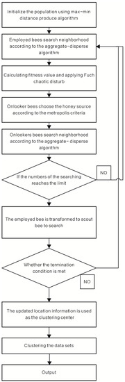
Figure 5.
Flow chart of Chaotic Adaptive Artificial Bee Colony-Kmeans.
- Initial parameters are set as follows: represents the number of population, denotes the space vector dimension, is the maximum iteration times, and cross parameter . is the threshold of maximum optimization times, and the annealing coefficient . The initial population is obtained according to the max–min distance product algorithm.
- The fitness value can be obtained according to Equation (3), and then solution approaches to the global optimal solution. At the same time, chaotic perturbations are added into the elite solution, which is selected from the preponderant solution set randomly and the infeasible solution in the bottom 15% according to Equation (16). The position is updated according to Equation (14) or Equation (15). Eventually, the location of the honey source is extended to the D-dimensional space. Whether the new solution is accepted depends on the Metropolis criteria.
- Onlooker bee executes the employed bee option and neighborhood searching performs under the same criteria.
- The updated location information, which is obtained after all the onlooker bees have completed the search, is used as the clustering center, the data set is performed a K-means iterative clustering, and the clustering center of each class is refreshed with the clustering division.
- If for abandonment is reached, the employed bee determines whether the number of updates reaches the limit. If the limit is reached, the employed bee is translated into a scout when the food source of which has been exhausted. A new round of honey source searching begins.
- If the number of iterations has reached the maximum “”, the optimal solution is output, otherwise, the algorithm goes back to step 2.
- K-means algorithm is executed to get results.
4. Numerical Experiments
In order to verify the effectiveness of CAABC, we design an optimization performance test on 20 benchmark functions. In order to make fair comparison, the parameter settings are referred as [35]. The algorithm is compared with the classic ABC, the Hybrid Artificial Bee Colony which proposed memory mechanisms (HABC) [34], the Improved Artificial Bee Colony which charges permutation as employed to represent the solutions (IABC) [36] and the DFSABC algorithm respectively. In order to verify the effectiveness of each component of the algorithm, CAABC-1 and CAABC-2 are also compared. The details of benchmark functions are listed in Table 1. In addition, we also use three standard evaluation index to evaluate the clustering performance of CAABC-K-means algorithm and other algorithms in this part.

Table 1.
Benchmark Function.
The simulation experiment is coded using MATLAB® R2019a, running on a system with 2.5 GHz Core-i5 CPU, 4 GB RAM, and Windows 10 operating system.
4.1. Test Environment and Parameter Settings
The experimental parameters are set as follows: dimensions are 30 and 60 respectively, and the maximum number of iterations is set to 15e4 and 30e4 respectively. In addition, the population size is set to 20 and the limit is set to . Under different dimension conditions, we run each benchmark function for 20 times independently.
4.2. CAABC Performance Analysis
To demonstrate the superiority and effectiveness of the CAABC, the CAABC algorithm is compared with other well-known algorithms on twenty benchmark problems. The population parameter settings are same as the setting mentioned in [36]: , the maximum number of evaluations , and other function parameter settings are shown in Table 2. Table 3 and Table 4 demonstrate the comparison under the 30-dimensional and 60-dimensional parameter settings respectively. The best results are shown in bold. All algorithms are executed in the same machine environment. Each result was recorded after separate trials for 20 times. The results are listed in Table 3 and Table 4; it can be clearly seen that most results of CAABC are remarkable in accuracy of convergence. Other algorithms are run with longer CPU time, which proves the superiority of CAABC algorithm. We select five representative test function for comparison, namely, Sphere (unimodal separable function US), Rosenbrock (unimodal nonseparable function UN), Rastrigin, Alpine (multimodal separable function MS) and Ackley (multimodal nonseparable function MN). The result is given in Figure 6 and Figure 7, which can make it visualized clearly from different views. In addition, the abscissa of the Figure 6 and 7 represents the number of iterations of the algorithm, the ordinate represents the value of the optimization function.
Table 2.
Parameter Setting.
Table 3.
Comparison with other improved Artificial Bee Colony in 30 dimensions.
Table 4.
Comparison with other improved Artificial Bee Colony in 60-dimensions.
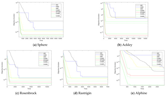
Figure 6.
Comparison with other improved Artificial Bee Colony algorithms in 30 dimensions.
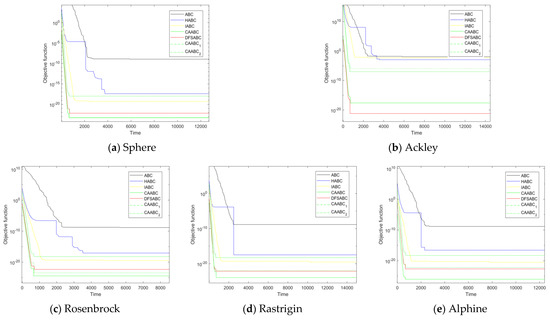
Figure 7.
Comparison with other improved Artificial Bee Colony algorithms in 60 dimensions.
According to the results in Table 3 and Table 4, it shows that CAABC is superior to or at least equal to other algorithms in the rest of benchmark functions except for the several benchmark functions. The case shown in Table 3 happens only on , and . In addition, in these functions, the difference between the improved algorithm and the others is less than 5%. However, in 60 dimensional comparison experiment, in Table 4, the improved algorithm achieves good results in . At the same time, it can be clearly seen in Figure 5 that CAABC also has a better convergence rate. Based on the above experimental sresults, the superiority of this algorithm is proved.
With the increase of dimension, the results of CAABC are even closer to ideal results. It indicates that the optimization effect of the CAABC is better than canonical ABC and other mentioned algorithms. The best value, the worst value, the average value, or the standard deviation, might be more ideal when the running time is basically the same. By comparing with CAABC-1 and CAABC-2, the effectiveness of the improved algorithm components has also been verified. Overall, compared with classic ABC and other improved ABC algorithms, the accuracy and efficiency of convergence have been enhanced. The exploration and exploitation performance are productively balanced at the same time.
4.3. CAABC-K-means Performance Analysis
The CAABC clustering algorithm on four standard evaluation indices are tested and compared with other well-known algorithms to evaluate the clustering performance of the proposed algorithm. To prove the clustering performance of the improved algorithm, in addition to the comparison algorithm mentioned above, experimental comparison with PA [35] and GPAM [37] clustering algorithm are also added. The general parameter setting is shown in Table 2. In addition, the maximum number of iterations is set to 100. The eleven datasets are Iris (7 January 1988), Balance-scale (22 April 1994), Wine (7 January 1991), E.coli (1 September 1996), Glass (9 January 1987), Abalone (12 January 1995), Musk (9 December 1994), Pendigits (7 January 1998), Skin Seg (17 July 2012), CMC (7 July 1997), and Cancer datasets (3 March 2017)(http://archive.ics.uci.edu/ml/). They have been considered to study and evaluate the performance of algorithms by many authors. The details of Iris, Balance-scale, Wine, E.coli, Glass, Abalone, Musk, Pendigits, Skin Seg, CMC, and Cancer datasets are summarized in Table 5. The optimal result is shown in bold in Table 6, Table 7, Table 8 and Table 9.
Table 5.
The datasets downloaded from UCI Machine Learning Repository.
Table 6.
The Normalized Mutual Information for classifying the eleven training datasets.
Table 7.
The Accuracy for classifying the eleven training datasets.
Table 8.
The average running time (sec.) for classifying the eleven training datasets.
Table 9.
The f-score of the training datasets.
We use standard evaluation index, Normalized Mutual Information (NMI), Accuracy (ACC), and F-score [38] to evaluate the clustering performance of CAABC-K-means algorithm and other algorithms. The corresponding results and the running time of the algorithm are analyzed in Table 6, Table 7, Table 8 and Table 9.
The NMI is defined as follows:
In the function, the is mutual information between the sample and the label and is the entropy.
In addition, the Accuracy (ACC) can be described as follow:
where is the number of samples, and is the correct number of samples.
In this paper, F-score is used to measure the accuracy of the clustering results. The performance comparisons among all the models are reported before and visualized in Table 9.
Precision (), Recall (), and F-measure () are often used to describe the accuracy of the clustering results. They are defined as follow:
where is True Positive, which is the number of the data that is classified into the cluster correctly. means False Negative, which is the number of the data that is not classified into the correct cluster. means False Positive, the number of the data that is classified into the cluster which is not belong. F-measure is the weighted harmonic average of Precision and Recall.
By analyzing the data of NMI, ACC, and running time from Table 6, Table 7 and Table 8, it is obvious that our proposed algorithm achieves excellent results than comparison algorithms. Specifically, Table 7 and Table 8 show that CAABC-K-means obtains a better accuracy of classification than most compared algorithms, and Table 6 and Table 8 show the proposed algorithm is more efficient and far superior to others. It is encouraging to find that CAABC-K-means achieves the highest F-core on ten datasets out of eleven datasets. The accuracy of the algorithm is better among the other clustering algorithms we compared with. Table 9 shows that the CAABC-K-means algorithm can offer a much better accuracy of classification than and similar efficiency to the traditional and some improved clustering algorithm.
From the above results, we can obtain that the CAABC algorithm performs better in terms of accuracy and efficiency. KMC algorithm is sensitive to initialization, so the computing time is longer, and it needs multiple iterations to reach the optimal value. ABC+K-means algorithm is easy to remain local optima, and it is difficult to achieve local optimization due to the stagnation of convergence in the later stage. The PSO+K-means and ABC_elite+K-means algorithms have improved the global optimization ability, however, the sensitivity of initialization of the clustering algorithm still exists, and the optimization effect of the algorithm is inconspicuous. Although the standard deviation has been reduced, the effect is inapparent. The improvement measures proposed in CAABC-K-means algorithm reduces the randomness in initializing, impairs the effect of an initial point, adaptive search mechanism to accelerate the algorithm convergence, and the disturbance and simulated annealing algorithm provide more possibility for solutions to escape from local optimum. Thus, the superiority of CAABC is obvious and the proposed algorithm can be considered as a feasible and efficient heuristic to find optimal solutions to clustering problems of allocating objects to K clusters.
5. Conclusions
Modeling the behavior of honey bees to search and solve problems has been the emerging area of swarm intelligence. In this paper, an improved artificial bee colony algorithm (CAABC) is developed to solve clustering problems. The method is inspired by the forage behavior in nature. The CAABC-K-means algorithm can be adapted to the process that the number of clusters known as a priori. In the CAABC algorithm, for the purpose of stabilizing the disturbance caused by the variety of the initial value of the clustering algorithm, we adapt the max–min distance product method in the initialization stage of the algorithm, which weakened the randomness of the initialization process to some extent. In the iterative process, chaotic disturbance and adaptive adjustment are added to obtain a better performance. After the comparison, chaos disturbance was added to the elite solution and unsatisfactory solutions in a certain percentage. The introduce of the “aggregate-disperse operation” speeds up the convergence of the algorithm and provides favorable conditions for escaping from the local optimal. Furthermore, on this basis, the global optimal solution is cross-operated to retain dominant individuals and improve population diversity. Moreover, the simulated annealing criterion is integrated into the probability selection to achieve a better precision. By selecting the appropriate functions, the characteristics of ABC for group optimization are retained, and the local optimal solution can be avoided effectively. In addition, CAABC-K-means has the global search ability of CAABC, which reduces the number of iterations of K-means. The problem of poor global search ability of Kmeans algorithm is solved by the combination of two algorithms. Furthermore, according to the characteristics of the clustering algorithm, the impacts of the sample numbers and the distance between the sample centers are took into account in fitness selection, which reduces the possibility that the distribution of samples is excessive clustered. To evaluate the performance of the confluent algorithm, it is compared with other stochastic heuristic algorithms on several benchmark functions and real datasets. It can be concluded from the primary results of experience, which are very promising in terms of the accuracy of the solution found and the processing efficiency, that the CAABC-K-means clustering algorithm achieves better results.
The efficiency and accuracy of the algorithm have been improved, but the time complexity cannot be reduced effectively because of the location update formula which is still guided by global optimal solution. How to ensure the advantages of the existing algorithm while reducing the time complexity will be our next research direction. Applying the proposed algorithm to solve other optimization problems and improving the performance of the clustering algorithm will be considered in our future work.
Author Contributions
All authors contributed extensively to the work presented in this paper. Conceptualization, Q.J. and N.L.; methodology, Q.J.; software, Q.J. and N.L.; validation, Q.J. and N.L.; formal analysis, N.L. and Y.Z.; investigation, Q.J., N.L. and Y.Z.; data curation, N.L.; writing—original draft preparation, N.L.; writing—review and editing, N.L. and Y.Z.; supervision, Q.J.; funding acquisition, Q.J. All authors have read and agreed to the published version of the manuscript.
Funding
This research was funded by National Natural Science Foundation of China, grant numbers 61673004 and the Fundamental Research Funds for the Central Universities of China (XK1802-4).
Institutional Review Board Statement
Not applicable.
Informed Consent Statement
Not applicable.
Data Availability Statement
Data sharing is not applicable to this article.
Conflicts of Interest
The authors declare no conflict of interest.
References
- Hartigan, J.A.; Wong, M.A. A K-Means Clustering Algorithm. Appl. Stat. 1979, 28, 100–108. [Google Scholar] [CrossRef]
- Punit, R.; Dheeraj, K.; Bezdek, J.C.; Sutharshan, R.; Palaniswami, M.S. A rapid hybrid clustering algorithm for large volumes of high dimensional data. IEEE Trans. Knowl. Data Eng. 2018, 31, 641–654. [Google Scholar]
- Ramadhani, F.; Zarlis, M.; Suwilo, S. Improve birch algorithm for big data clustering. IOP Conf. Ser. Mater. Sci. Eng. 2020, 725, 012090. [Google Scholar] [CrossRef]
- Cerreto, F.; Nielsen, B.F.; Nielsen, O.A.; Harrod, S.S. Application of data clustering to railway delay pattern recognition. J. Adv. Transp. 2018, 377–394. [Google Scholar] [CrossRef]
- Kouta, T.; Cullell-Dalmau, M.; Zanacchi, F.C.; Manzo, C. Bayesian analysis of data from segmented super-resolution images for quantifying protein clustering. Phys. Chem. Chem. Phys. 2020, 22, 1107–1114. [Google Scholar] [CrossRef] [PubMed]
- Dhifli, W.; Karabadji NE, I.; Elati, M. Evolutionary mining of skyline clusters of attributed graph data. Inf. Sci. 2020, 509, 501–514. [Google Scholar] [CrossRef]
- Eberhart, S.Y. Particle swarm optimization: Developments, applications and resources. In Proceedings of the Congress on Evolutionary Computation, Seoul, Korea, 27–30 May 2001. [Google Scholar]
- Xiang, W.L.; Li, Y.Z.; He, R.C.; Gao, M.X.; An, M.Q. A novel artificial bee colony algorithm based on the cosine similarity. Comput. Ind. Eng. 2018, 115, 54–68. [Google Scholar] [CrossRef]
- Karaboga, D. An Idea Based on Honey bee Swarm for Numerical Optimization; Technical Report-tr06; Erciyes University: Kayseri, Turkiye, 2005. [Google Scholar]
- Zhang, X.; Zhang, X.; Ho, S.L.; Fu, W.N. A modification of artificial bee colony algorithm applied to loudspeaker design problem. IEEE Trans. Magn. 2014, 50, 737–740. [Google Scholar] [CrossRef]
- Zhu, G.; Kwong, S. Gbest-guided artificial bee colony algorithm for numerical function optimization. Appl. Math. Comput. 2010, 217, 3166–3173. [Google Scholar] [CrossRef]
- Zhang, P.H.; Jing-Ming, L.I.; Xian-De, H.U.; Jun, H.U. Research on global artificial bee colony algorithm based on crossover. J. Shandong Univ. Technol. 2017, 11, 1672–6197. [Google Scholar]
- Cui, L.; Li, G.; Lin, Q.; Du, Z.; Gao, W.; Chen, J. A novel artificial bee colony algorithm with depth-first search framework and elite-guided search equation. Inf. Sci. 2016, 367–368, 1012–1044. [Google Scholar] [CrossRef]
- Sharma, T.K.; Pant, M. Enhancing Scout Bee Movements in Artificial Bee Colony Algorithm. In Proceedings of the International Conference on Soft Computing for Problem Solving, Roorkee, India, 20–22 December 2011. [Google Scholar]
- Yang, Z.; Gao, H.; Hu, H. Artificial bee colony algorithm based on self-adaptive greedy strategy. In Proceedings of the IEEE International Conference on Advanced Computational Intelligence, Xiamen, China, 29–31 March 2018; pp. 385–390. [Google Scholar]
- Gao, W.; Liu, S.; Huang, L. A global best artificial bee colony algorithm for global optimization. J. Comput. Appl. Math. 2012, 236, 2741–2753. [Google Scholar] [CrossRef]
- Gao, W.; Liu, S.; Huang, L. A novel artificial bee colony algorithm with Powell’s method. Appl. Soft Comput. 2013, 13, 3763–3775. [Google Scholar] [CrossRef]
- Wu, B.; Qian, C.; Ni, W.; Fan, S. Hybrid harmony search and artificial bee colony algorithm for global optimization problems. Comput. Math. Appl. 2012, 64, 2621–2634. [Google Scholar] [CrossRef]
- Kang, F.; Li, J.; Li, H. Artificial bee colony algorithm and pattern search hybridized for global optimization. Appl. Soft Comput. 2013, 13, 1781–1791. [Google Scholar] [CrossRef]
- Tasgetiren, M.F.; Pan, Q.K.; Suganthan, P.N.; Chen, H.L. A discrete artificial bee colony algorithm for the total flowtime minimization in permutation flow shops. Inf. Sci. 2011, 181, 3459–3475. [Google Scholar] [CrossRef]
- Guanlong, D.; Zhenhao, X.; Xingsheng, G. A Discrete Artificial Bee Colony Algorithm for Minimizing the Total Flow Time in the Blocking Flow Shop Scheduling. Chin. J. Chem. Eng. 2012, 20, 1067–1073. [Google Scholar]
- Zhang, R.; Song, S.; Wu, C. A hybrid artificial bee colony algorithm for the job shop scheduling problem. Int. J. Prod. Econ. 2013, 141, 167–178. [Google Scholar] [CrossRef]
- Pan, Q.K.; Wang, L.; Li, J.Q.; Duan, J.H. A novel discrete artificial bee colony algorithm for the hybrid flowshop scheduling problem with makespan minimisation. Omega 2014, 45, 42–56. [Google Scholar] [CrossRef]
- Gao, K.Z.; Suganthan, P.N.; Pan, Q.K.; Tasgetiren, M.F.; Sadollah, A. Artificial bee colony algorithm for scheduling and rescheduling fuzzy flexible job shop problem with new job insertion. Knowl. Based Syst. 2016, 109, 1–16. [Google Scholar] [CrossRef]
- Li, J.Q.; Pan, Q.K. Solving the Large-Scale Hybrid Flow Shop Scheduling Problem with Limited Buffers by a Hybrid Artificial Bee Colony Algorithm; Elsevier Science Inc.: Beijing, China, 2015. [Google Scholar]
- Liu, J.; Meng, L.-Z. Integrating Artificial Bee Colony Algorithm and BP Neural Network for Software Aging Prediction in IoT Environment. IEEE Access 2019, 7, 32941–32948. [Google Scholar] [CrossRef]
- Karaboga, D.; Gorkemli, B. A quick artificial bee colony -qABC- algorithm for optimization problems. In Proceedings of the 2012 International Symposium on Innovations in Intelligent Systems and Applications, Trabzon, Turkey, 2–4 July 2012. [Google Scholar]
- Zaragoza, J.C.; Sucar, E.; Morales, E.; Bielza, C.; Larranaga, P. Bayesian Chain Classifiers for Multidimensional Classification. In Proceedings of the International Joint Conference on Ijcai, Catalonia, Spain, 16–22 July 2011. [Google Scholar]
- Park, J.Y.; Han, S.Y. Application of artificial bee colony algorithm to topology optimization for dynamic stiffness problems. Comput. Math. Appl. 2013, 66, 1879–1891. [Google Scholar] [CrossRef]
- Xiang, Y.; Zhou, Y. A dynamic multi-colony artificial bee colony algorithm for multi-objective optimization. Appl. Soft Comput. 2015, 35, 766–785. [Google Scholar] [CrossRef]
- Borchani, H.; Bielza, C.; Larranaga, P. Learning CB-decomposable multi-dimensional bayesian network classifiers. In Proceedings of the 5th European Workshop on Probabilistic Graphical Models, Helsinki, Finland, 13–15 September 2010; pp. 25–32. [Google Scholar]
- Lou, A. A Fusion Clustering Algorithm Based on Global Gravitation Search and Partitioning Around Medoid. In Proceedings of the CSSE 2019: Proceedings of the 2nd International Conference on Computer Science and Software Engineering, Rome, Italy, 22–23 June 2019; p. 6. [Google Scholar]
- Wu, M. Heuristic parallel selective ensemble algorithm based on clustering and improved simulated annealing. J. Supercomput. 2018, 76, 3702–3712. [Google Scholar] [CrossRef]
- Fan, C. Hybrid artificial bee colony algorithm with variable neighborhood search and memory mechanism. J. Syst. Eng. Electron. 2018, 29, 405–414. [Google Scholar] [CrossRef]
- Tellaroli, P. CrossClustering: A Partial Clustering Algorithm. PLoS ONE 2018, 11, e0152333. [Google Scholar]
- Peng, K.; Pan, Q.K.; Zhang, B. An Improved Artificial Bee Colony Algorithm for Steelmaking-refining-Continuous Casting Scheduling Problem. Chin. J. Chem. Eng. 2018, 26, 1727–1735. [Google Scholar] [CrossRef]
- Wenyuan, F.U.; Chaodong, L. An Adaptive Iterative Chaos Optimization Method. J. Xian Jiaotong Univ. 2013, 47, 33–38. [Google Scholar]
- Yu, S.-S.; Chu, S.-W.; Wang, C.-M.; Chan, Y.-K.; Chang, T.-C. Two improved k-means algorithms. Appl. Soft Comput. 2018, 68, 747–755. [Google Scholar] [CrossRef]


Publisher’s Note: MDPI stays neutral with regard to jurisdictional claims in published maps and institutional affiliations. |
© 2021 by the authors. Licensee MDPI, Basel, Switzerland. This article is an open access article distributed under the terms and conditions of the Creative Commons Attribution (CC BY) license (http://creativecommons.org/licenses/by/4.0/).