
GW-DC: A Deep Clustering Model Leveraging Two-Dimensional Image Transformation and Enhancement

Abstract
:1. Introduction
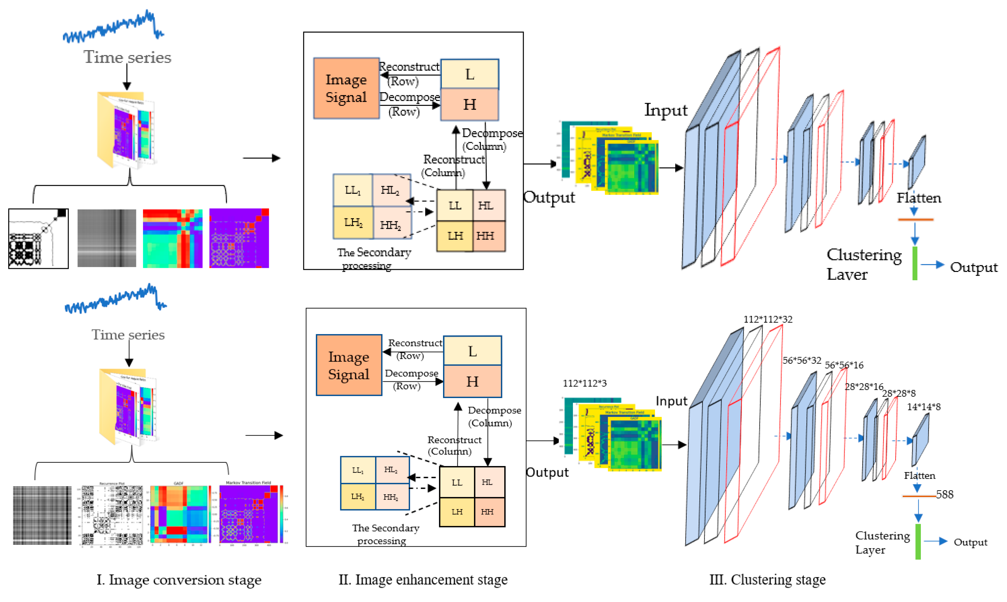
2. Methodology
2.1. Image Conversion Stage
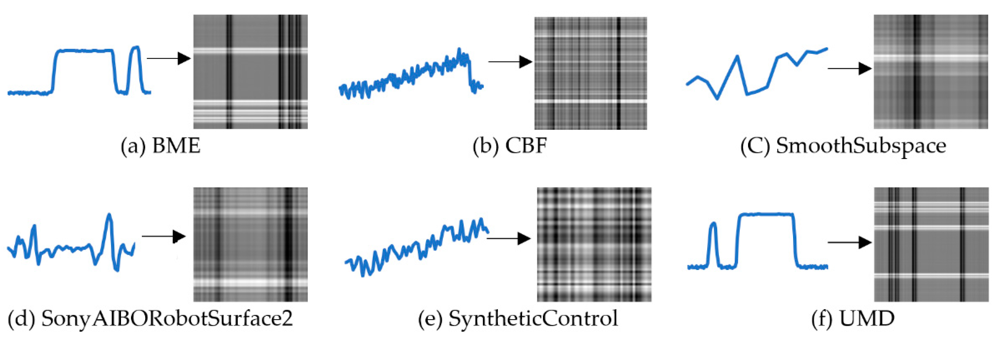
2.1.1. Conversion from Time-Series into Grayscale Image
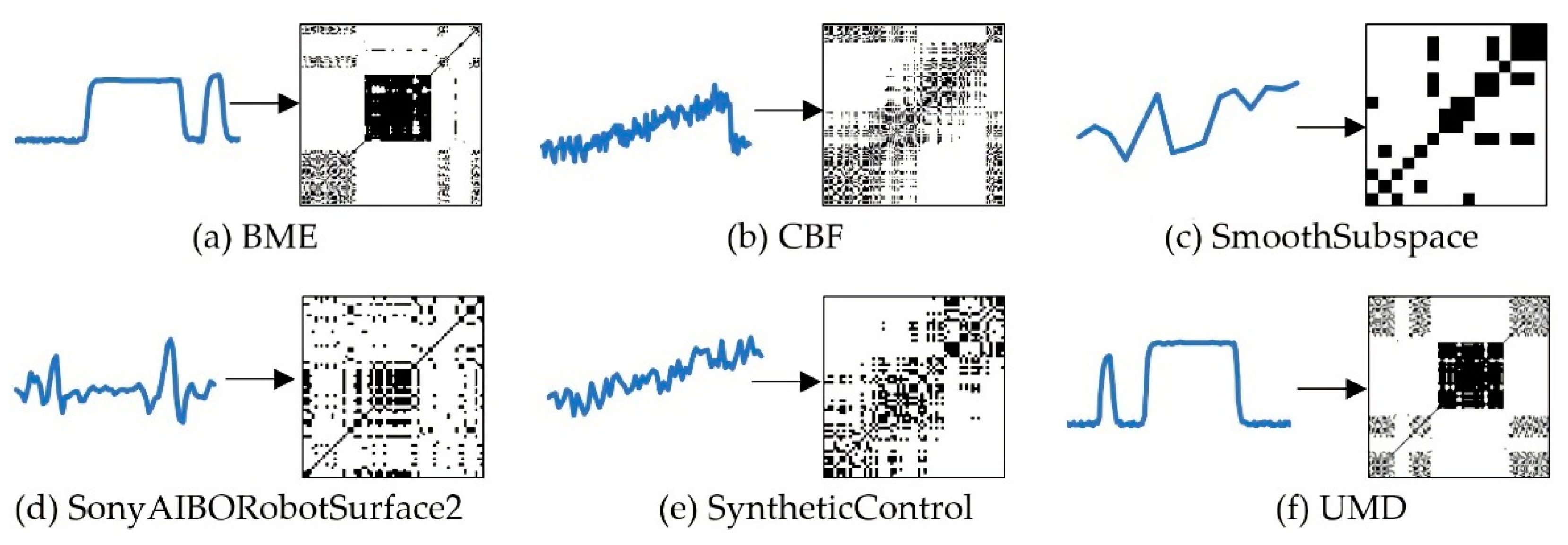
2.1.2. Conversion from Time-Series into RP Images
2.1.3. Conversion from Time-Series into MTF Images
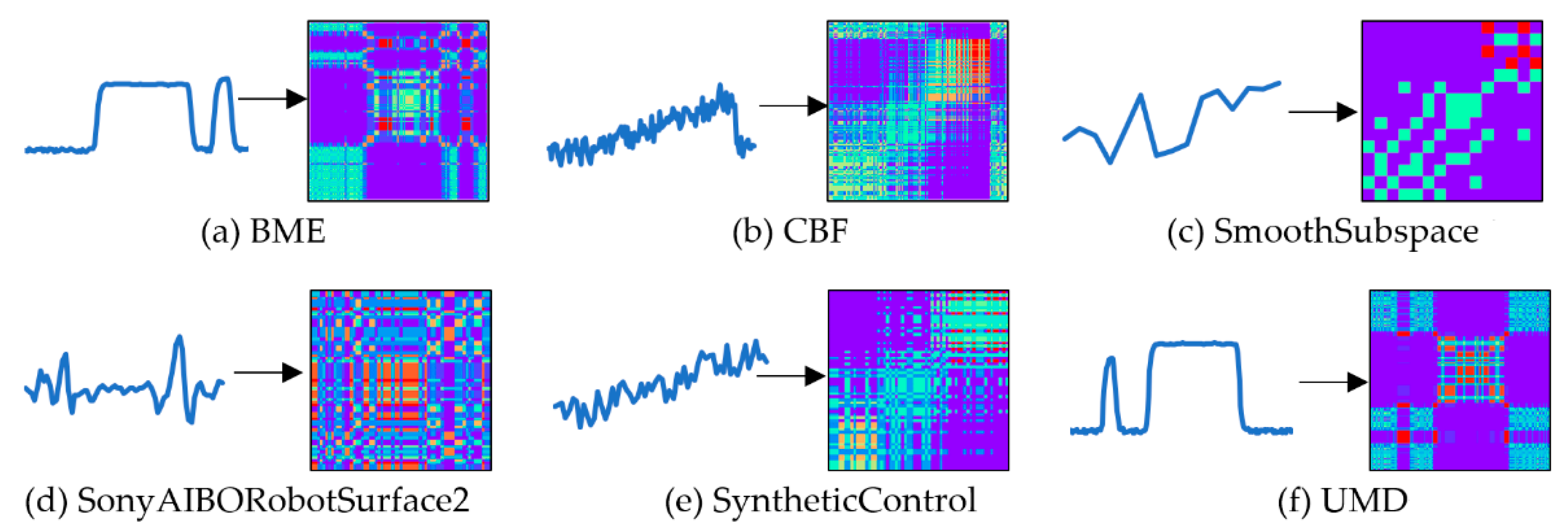
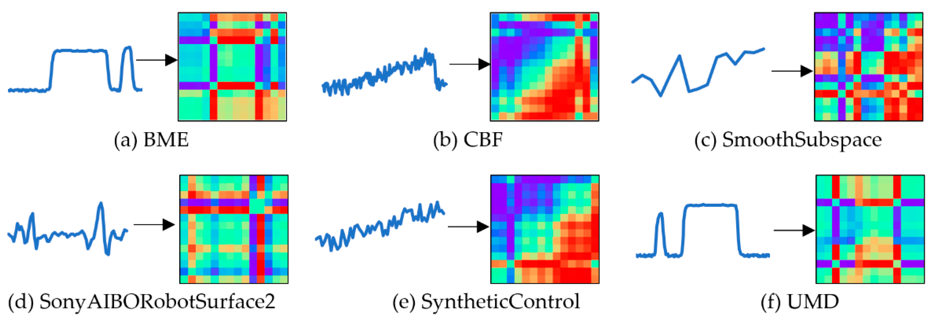
2.1.4. Conversion from Time-Series to Gramian Angular Difference Field
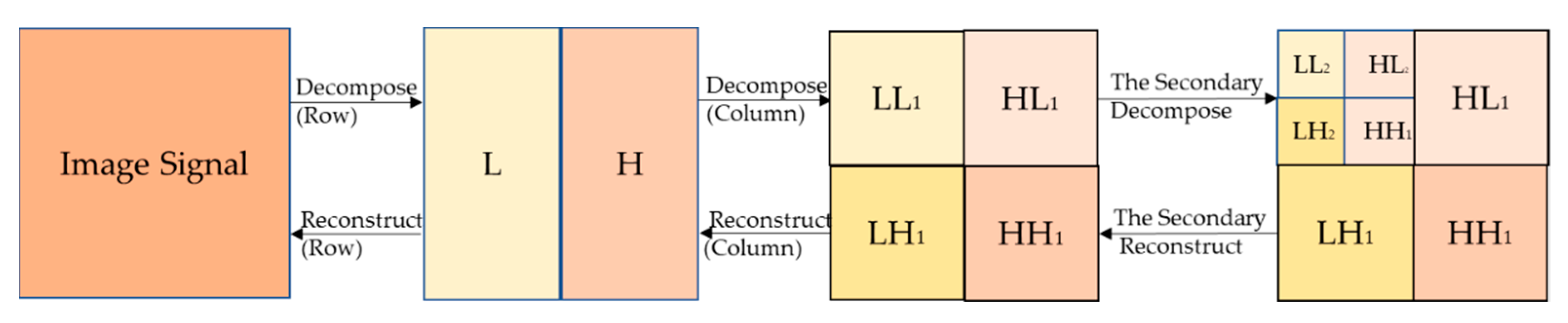
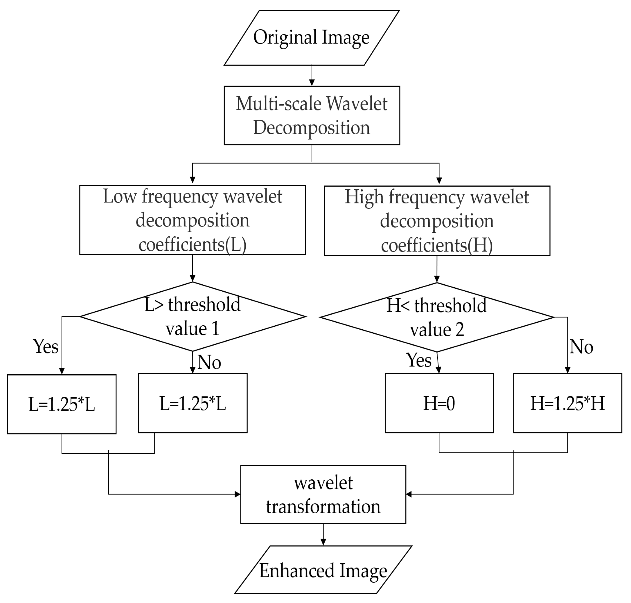
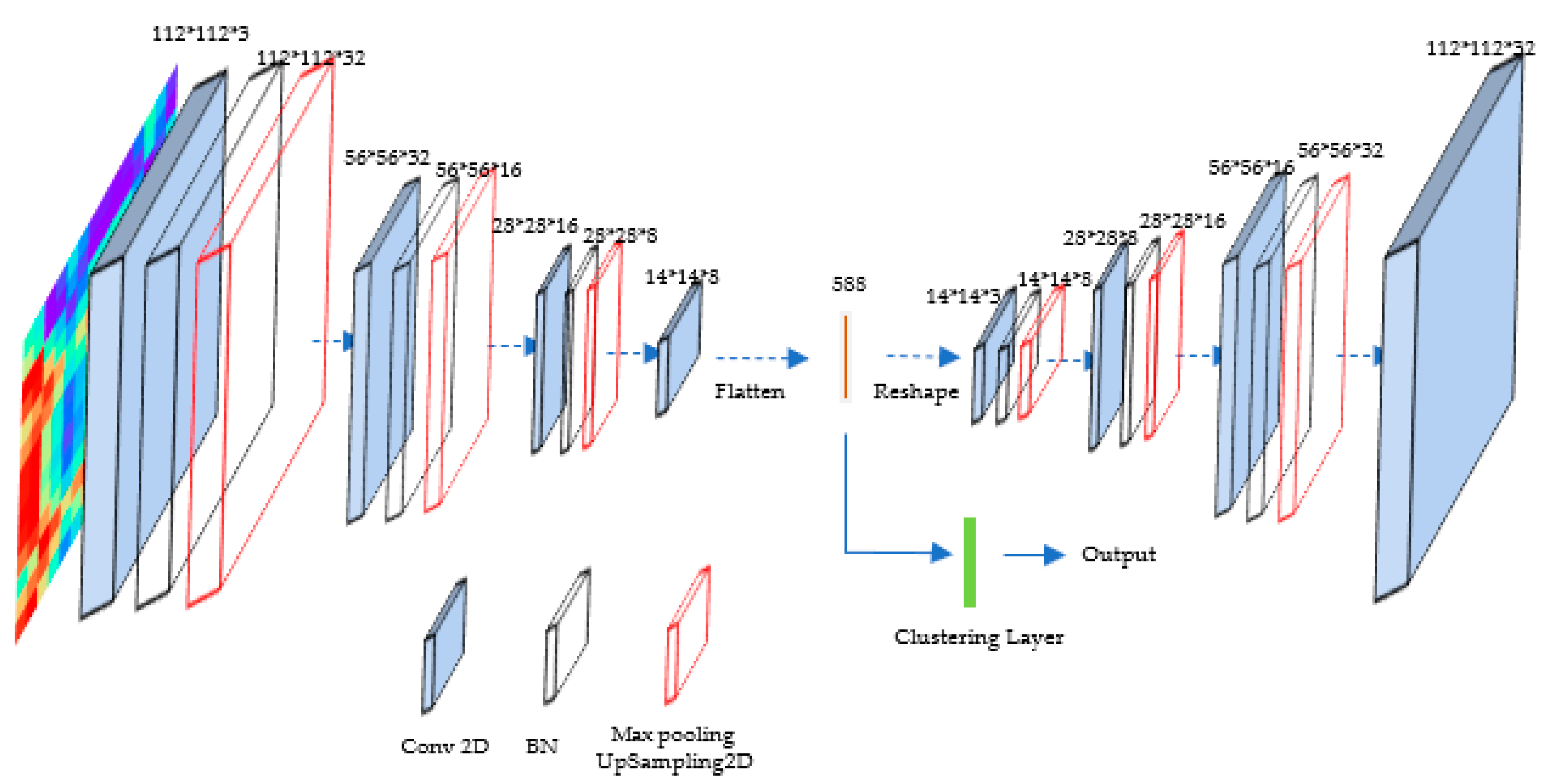
2.2. Image Enhancement Stage
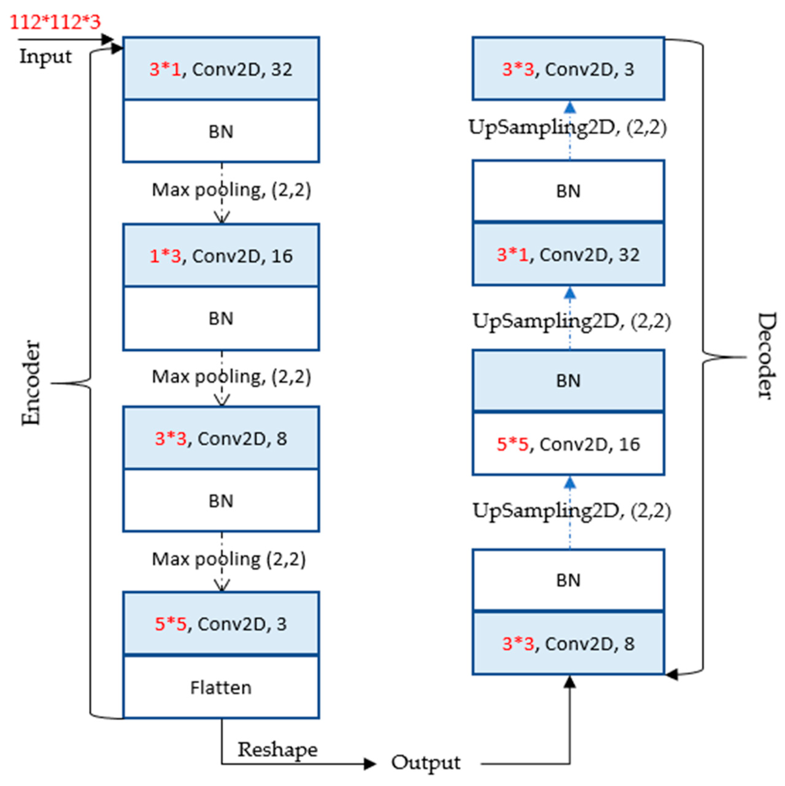
2.3. Image Clustering Stage
3. Experiment and Results
3.1. Datasets and Evaluation Index
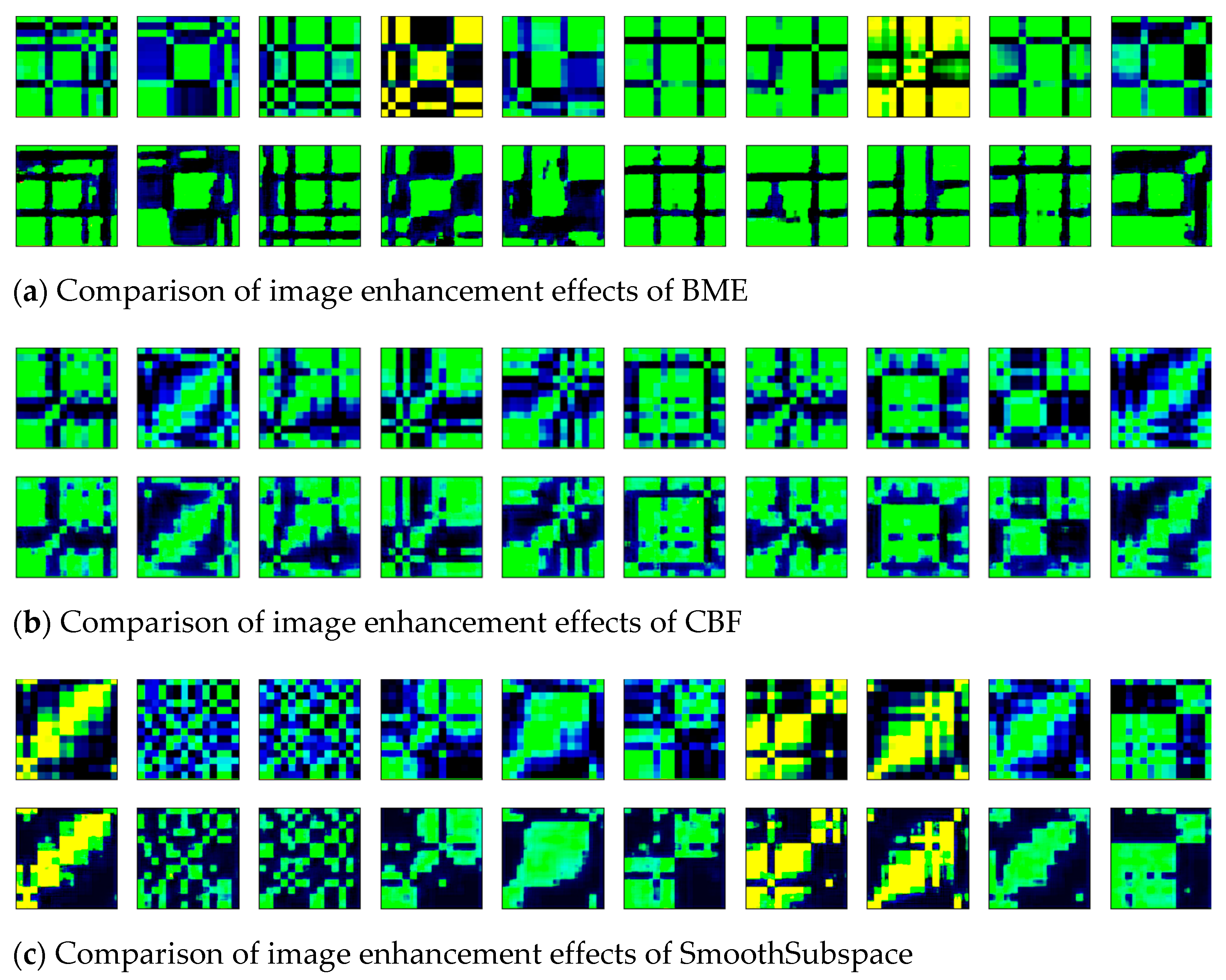
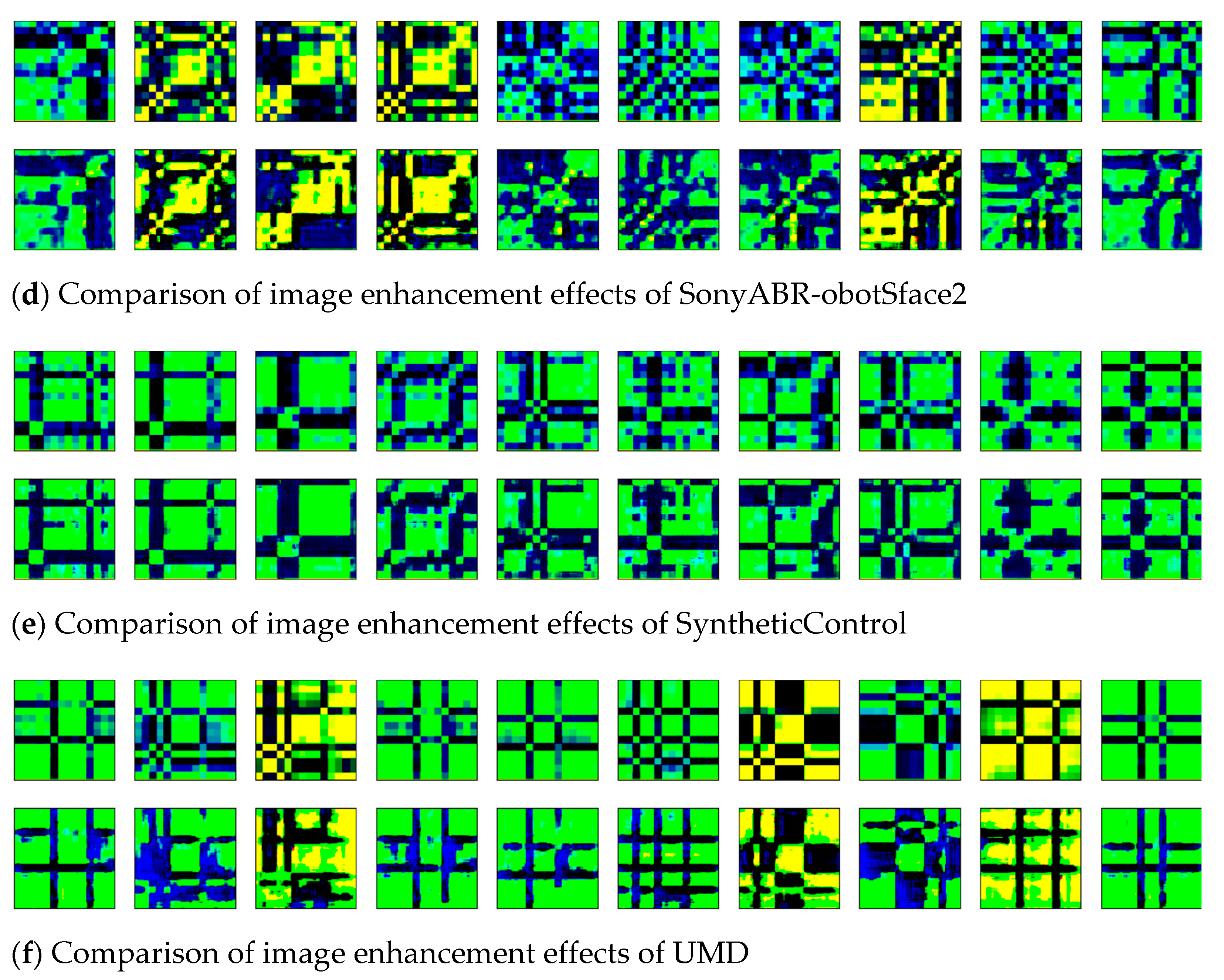
3.2. Conversion Result of Two-Dimensional Images
3.3. Comparative Analysis of Clustering Results
4. Conclusions
Author Contributions
Funding
Institutional Review Board Statement
Informed Consent Statement
Data Availability Statement
Conflicts of Interest
References
- Li, H.L. Multivariate time series clustering based on common principal component analysis. Neurocomputing 2019, 349, 239–247. [Google Scholar] [CrossRef]
- Chira, C.; Sedano, J.; Camara, M.; Prieto, C.; Villar, J.R.; Corchado, E. A cluster merging method for time series microarray with production values. Int. J. Neural Syst. 2014, 24, 1450018. [Google Scholar] [CrossRef] [PubMed]
- Karim, F.; Majumdar, S.; Darabi, H.; Chen, S. LSTM fully convolutional networks for time series classification. IEEE Access 2018, 6, 1662–1669. [Google Scholar] [CrossRef]
- Gao, Y.P.; Chang, D.F.; Fang, T.; Fan, Y.Q. The Daily Container Volumes Prediction of Storage Yard in Port with Long Short-Term Memory Recurrent Neural Network. Available online: https://www.hindawi.com/journals/jat/2019/5764602/ (accessed on 15 November 2021).
- Li, H.T.; Bai, J.C.; Li, Y.W. A novel secondary decomposition learning paradigm with kernel extreme learning machine for multi-step forecasting of container throughput. Physica A 2019, 534, 122025. [Google Scholar] [CrossRef]
- Liao, T.W. Clustering of time series data—A survey. Pattern Recognit. 2005, 38, 1857–1874. [Google Scholar] [CrossRef]
- Huang, X.H.; Ye, Y.M.; Xiong, L.Y.; Lau, R.Y.K.; Jiang, N.; Wang, S.K. Time series k-means: A new k-means type smooth subspace clustering for time series data. Inf. Sci. 2016, 367, 1–13. [Google Scholar] [CrossRef]
- Guijo-Rubio, D.; Duran-Rosal, A.M.; Gutierrez, P.A.; Troncoso, A.; Hervas-Martinez, C. Time-Series Clustering Based on the Characterization of Segment Typologies. IEEE Trans. Cybern. 2020, 51, 2962584. [Google Scholar] [CrossRef]
- Zhang, Y.P.; Qu, H.; Wang, W.P.; Zhao, J.H. A Novel Fuzzy Time Series Forecasting Model Based on Multiple Linear Regression and Time Series Clustering. Available online: https://www.hindawi.com/journals/mpe/2020/9546792/ (accessed on 15 November 2021).
- Hung, W.L.; Yang, M.S. Similarity measures of intuitionistic fuzzy sets based on Hausdorff distance. Pattern Recognit. Lett. 2004, 25, 1603–1611. [Google Scholar] [CrossRef]
- Xu, H.; Zeng, W.H.; Zeng, X.X.; Yen, G.G. An evolutionary algorithm based on Minkowski distance for many-objective optimization. IEEE T. Cybern. 2019, 49, 3968–3979. [Google Scholar] [CrossRef]
- Ioannidou, Z.S.; Theodoropoulou, M.C.; Papandreou, N.C.; Willis, J.H.; Hamodrakas, S.J. CutProtFam-Pred: Detection and classification of putative structural cuticular proteins from sequence alone, based on profile hidden Markov models. Insect Biochem. Mol. Biol. 2014, 52, 51–59. [Google Scholar] [CrossRef] [Green Version]
- Liu, H.C.; Liu, L.; Li, P. Failure mode and effects analysis using intuitionistic fuzzy hybrid weighted Euclidean distance operator. Int. J. Syst. Sci. 2014, 45, 2012–2030. [Google Scholar] [CrossRef]
- Guan, X.D.; Huang, C.; Liu, G.H.; Meng, X.L.; Liu, Q.S. Mapping rice cropping systems in Vietnam using an NDVI-based time-series similarity measurement based on DTW distance. Remote Sens. 2016, 8, 19. [Google Scholar] [CrossRef] [Green Version]
- Wang, J.; Wu, J.; Ni, J.; Chen, J.; Xi, C. Relationship between Urban Road Traffic Characteristics and Road Grade Based on a Time Series Clustering Model: A Case Study in Nanjing, China. Chin. Geogr. Sci. 2018, 28, 1048–1060. [Google Scholar] [CrossRef] [Green Version]
- Yang, B.; Fu, X.; Sidiropoulos, N.D.; Hong, M.Y. Towards K-means-friendly Spaces: Simultaneous Deep Learning and Clustering. In Proceedings of the 34th International Conference on Machine Learning (ICML), Sydney, Australia, 6–11 August 2017. [Google Scholar]
- Huang, P.H.; Huang, Y.; Wang, W.; Wang, L. Deep Embedding Network for Clustering. In Proceedings of the 22nd International Conference on Pattern Recognition (ICPR), Stockholm, Sweden, 24–28 August 2014. [Google Scholar]
- Ji, P.; Zhang, T.; Li, H.D.; Salzmann, M.; Reid, I. Deep subspace clustering networks. In Proceedings of the 31st Annual Conference on Neural Information Processing Systems (NIPS), Long Beach, CA, USA, 4–9 December 2017. [Google Scholar]
- Chen, D.; Lv, J.C.; Yi, Z. Unsupervised multi-manifold clustering by learning deep representation. In Proceedings of the 31st AAAI Conference on Artificial Intelligence (AAAI), San Francisco, CA, USA, 4–9 February 2017. [Google Scholar]
- Lee, H.; Grosse, R.; Ranganath, R.; Ng, A.Y. Convolutional deep belief networks for scalable unsupervised learning of hierarchical representations. In Proceedings of the 26th Annual International Conference on Machine Learning, Montreal, ON, Canada, 14–18 June 2009. [Google Scholar]
- Chen, J. Deep Learning with Nonparametric Clustering. arXiv 2015, arXiv:1501.03084. Available online: https://arxiv.org/abs/1501.03084 (accessed on 15 November 2021).
- Xie, J.; Girshick, R.; Farhadi, A. Unsupervised Deep Embedding for Clustering Analysis. arXiv 2016, arXiv:1511.06335. Available online: https://arxiv.org/abs/1511.06335 (accessed on 15 November 2021).
- Li, F.F.; Qiao, H.; Zhang, B. Discriminatively boosted image clustering with fully convolutional auto-encoders. Pattern Recognit. 2018, 83, 161–173. [Google Scholar] [CrossRef] [Green Version]
- Goodfellow, I.J.; Pouget-Abadie, J.; Mirza, M.; Xu, B.; Warde-Farley, D.; Ozair, S.; Courville, A.; Bengio, Y. Generative adversarial nets. Adv. Neural Inf. Process. Syst. 2014, 27, 2672–2680. [Google Scholar]
- Jiang, Z.; Zheng, Y.; Tan, H.; Tang, B.; Zhou, H. Variational Deep Embedding: An Unsupervised and Generative Approach to Clustering. arXiv 2016, arXiv:1611.05148. Available online: https://arxiv.org/abs/1611.05148 (accessed on 15 November 2021).
- Chang, J.; Wang, L.; Meng, G.; Xiang, S.; Pan, C. Deep adaptive image clustering. In Proceedings of the 2017 IEEE International Conference on Computer Vision (ICCV), Venice, Italy, 22–29 October 2017. [Google Scholar]
- Liu, L.Z.; Qian, X.Y.; Lu, H.Y. Cross-sample entropy of foreign exchange time series. Physica A 2010, 389, 4785–4792. [Google Scholar] [CrossRef]
- Chen, W.; Shi, K. A deep learning framework for time series classification using Relative Position Matrix and Convolutional Neural Network. Neurocomputing 2019, 359, 384–394. [Google Scholar] [CrossRef]
- Szegedy, C.; Vanhoucke, V.; Loffe, S.; Shlens, J.; Wojna, Z. Rethinking the Inception Architecture for Computer Vision. In Proceedings of the 2016 IEEE Conference on Computer Vision and Pattern Recognition (CVPR), Las Vegas, NV, USA, 27–30 June 2016. [Google Scholar]
- Contreras-Reyes, J.E. Mutual information matrix based on asymmetric Shannon entropy for nonlinear interactions of time series. Nonlinear Dyn. 2021, 104, 3913–3924. [Google Scholar] [CrossRef]
- Tian, F.; Gao, B.; Cui, Q.; Chen, E.H.; Liu, T.Y. Learning Deep Representations for Graph Clustering. In Proceedings of the 28th AAAI Conference on Artificial Intelligence (AAAI), Quebec City, QC, Canada, 27–31 July 2014. [Google Scholar]
- Song, C.F.; Liu, F.; Huang, Y.Z.; Wang, L.; Tan, T.N. Auto-Encoder Based Data Clustering; Springer: Berlin/Heidelberg, Germany, 2013. [Google Scholar]

| Dataset | Description | Train Size | Test Size | Length | Classes |
|---|---|---|---|---|---|
| BME | Beef spectrograms, from pure beef and beef adulterated with varying degrees of offal. | 30 | 150 | 128 | 3 |
| CBF | The data for each class is standard normal noise plus different offset terms. | 30 | 900 | 128 | 3 |
| SmoothSubspace | Each time-series contains a continuous subspace spanning 5 continuous timestamps, which is used to test whether smooth subspace can be extracted. | 150 | 150 | 15 | 3 |
| SonyAIBORobotSurface2 | This dataset contains different accelerometers for robot walking in cement or carpet/field. | 27 | 953 | 65 | 2 |
| SyntheticControl | Six different categories of control charts, including normal, cyclic, increasing trend, decreasing trend, upward shift, and downward shift. | 300 | 300 | 60 | 6 |
| UMD | A synthetic dataset with three types: upper, lower, and no bells arising at the initial or final cycle. | 36 | 144 | 150 | 3 |
| Image Type | BME | CBF | SmoothSubspace | SonyABR-obotSface2 | SyntheticControl | UMD |
|---|---|---|---|---|---|---|
| Grayscale | 91.18 | 44.32 | 22.89 | 23.50 | 26.26 | 41.50 |
| RP | 33.14 | 58.30 | 39.13 | 27.12 | 65.63 | 33.93 |
| MTF | 38.54 | 53.26 | 12.74 | 21.88 | 51.08 | 12.29 |
| GADF | 91.18 | 54.77 | 42.43 | 25.74 | 71.45 | 46.53 |
| Dataset | SAE +K-Means [31] | AE +K-Means [32] | AE_Conv +K-Means | |||
| Index | NMI | ACC | NMI | ACC | NMI | ACC |
| BME | 22.37 | 55.56 | 20.62 | 50.69 | 16.27 | 55.56 |
| CBF | 27.69 | 51.08 | 23.24 | 48.39 | 26.89 | 58.47 |
| SmoothSubspce | 6.21 | 50.00 | 8.13 | 50.83 | 19.64 | 75.00 |
| SonyAIBORobotSurface2 | 24.29 | 71.43 | 0.19 | 67.22 | 13.34 | 64.29 |
| SyntheticControl | 35.71 | 47.50 | 15.68 | 28.12 | 15.78 | 39.58 |
| UMD | 26.78 | 52.78 | 14.30 | 46.53 | 18.63 | 55.56 |
| Dataset | DEC [22] | DEC_FCN | GW_DC | |||
| Index | NMI | ACC | NMI | ACC | NMI | ACC |
| BME | 46.69 | 58.33 | 44.54 | 52.78 | 91.18 | 61.13 |
| CBF | 30.32 | 76.88 | 32.77 | 63.44 | 54.77 | 80.65 |
| SmoothSubspce | 28.01 | 53.33 | 23.37 | 51.67 | 42.43 | 65.00 |
| SonyAIBORobotSurface2 | 30.17 | 79.08 | 14.30 | 76.02 | 25.74 | 77.04 |
| SyntheticControl | 24.72 | 53.33 | 52.82 | 40.00 | 71.45 | 66.67 |
| UMD | 33.74 | 63.89 | 16.46 | 66.67 | 46.53 | 75.00 |
Publisher’s Note: MDPI stays neutral with regard to jurisdictional claims in published maps and institutional affiliations. |
© 2021 by the authors. Licensee MDPI, Basel, Switzerland. This article is an open access article distributed under the terms and conditions of the Creative Commons Attribution (CC BY) license (https://creativecommons.org/licenses/by/4.0/).
Share and Cite
Li, X.; Li, T.; Wang, Y. GW-DC: A Deep Clustering Model Leveraging Two-Dimensional Image Transformation and Enhancement. Algorithms 2021, 14, 349. https://doi.org/10.3390/a14120349
Li X, Li T, Wang Y. GW-DC: A Deep Clustering Model Leveraging Two-Dimensional Image Transformation and Enhancement. Algorithms. 2021; 14(12):349. https://doi.org/10.3390/a14120349
Chicago/Turabian StyleLi, Xutong, Taoying Li, and Yan Wang. 2021. "GW-DC: A Deep Clustering Model Leveraging Two-Dimensional Image Transformation and Enhancement" Algorithms 14, no. 12: 349. https://doi.org/10.3390/a14120349
APA StyleLi, X., Li, T., & Wang, Y. (2021). GW-DC: A Deep Clustering Model Leveraging Two-Dimensional Image Transformation and Enhancement. Algorithms, 14(12), 349. https://doi.org/10.3390/a14120349