Autoencoder-Based Reduced Order Observer Design for a Class of Diffusion-Convection-Reaction Systems

Abstract

The application of autoencoders in combination with Dynamic Mode Decomposition for control (DMDc) and reduced order observer design as well as Kalman Filter design is discussed for low order state reconstruction of a class of scalar linear diffusion-convection-reaction systems. The general idea and conceptual approaches are developed following recent results on machine-learning based identification of the Koopman operator using autoencoders and DMDc for finite-dimensional discrete-time system identification. The resulting linear reduced order model is combined with a classical Kalman Filter for state reconstruction with minimum error covariance as well as a reduced order observer with very low computational and memory demands. The performance of the two schemes is evaluated and compared in terms of the approximated $L^2$ error norm in a numerical simulation study. It turns out, that for the evaluated case study the reduced-order scheme achieves comparable performance with significantly less computational load.

1. Introduction

The problem of system state reconstruction from local and partial state measurements has important impacts on the ability of controlling the system state and monitoring system health and performance [1,2,3]. This becomes particularly involved in the framework of spatially continuously distributed dynamical systems, which are typically modeled using partial differential equations (pdes). The so called associated state estimation or observer design problem has been studied over the last decades and already reached a state of maturity in particular for linear systems (see, e.g., [4,5]). Additionally, for some classes of nonlinear or semilinear systems, design approaches have been obtained, which differ in design complexity and computational load in their implementation. A particular approach, which is simple and can be implemented with small computational load is the pointwise measurement injection (or pointwise innovation) observer design, which has been employed for solving the problem for some types of semilinear parabolic problems [6,7,8,9,10]. This approach basically extends the idea of a reduced order observer design [1,2] to the considered class of infinite-dimensional systems. The reduced order property is to be understood in relation to the number of internal states of the observer in comparison to the number of states in the system to be monitored. Basically the idea consists in providing a non-redundant state estimation scheme, which does not need to estimate the measured output, but only non-measured state variables.

Considering pde models leads to the additional problem that for implementing any observer in a real-time monitoring scheme, the associated set of pdes has to be solved numerically. This is done using some kind of discretization in space and time, so that a finite-dimensional discrete-time system representation is obtained, which represents a digital twin of the original pde system. The number of internal state variables of this approximation model is typically very high (from about hundred to several thousands of variables, e.g., for finite-element approximations) and thus requires model-order reduction approaches for real-time applicability. For this purpose, typically balanced truncation or proper orthogonal decomposition approaches or similar are employed (see, e.g., [11] and references therein). Besides these, in recent years a focus was led to approaches using dynamic mode decomposition (DMD) [11,12] and its extension to DMDc to include external (control) inputs [13]. The usage of DMD (or DMDc) is particularly motivated by the Koopman theory, according to which nonlinear finite-dimensional systems can be embedded into an infinite-dimensional space on which the linear Kooppman operator provides a complete description of the time evolution of the system observables. The (Koopman) eigenfunctions or the associated Koopman operator form a basis of this space and can be used in principle to determine a finite-dimensional approximation of the dominant modes of this operator (associated to the dominant eigenvalues of the operator). As this embedding can in most cases not be carried out analytically (see, e.g., the discussion in [3,11,12]) one can employ DMD (or DMDc) as a data-based identification approach using snapshots of the state observables as training data. This idea has been combined with the use of autoencoders (AEs) to learn from the training data a low-dimensional basis of the associated dominant Koopman eigenfunction subspace in which a linear dynamics can then be identified using classical DMDc [14]. The use of autoencoders and Koopman theory for automatic learning of finite-dimensional system dynamics is also mainstream in contemporary control systems applications in general (see, e.g., [15,16]).

Having finite-dimensional approximations of the infinite-dimensional pde models, one can also directly address the observer design problem in the finite-dimensional setup. This approach is also called early lumping (first approximate and then design), while the results discussed before belong to the so-called late lumping (first design then approximate) approaches.

Early lumping based on the combination of DMDc with state estimation has already been shown in several application scenarios to yield satisfactory performance [3,17,18,19,20]. In these studies the Kalman Filter [21,22] has been used on the basis of the obtained finite-dimensional linear discrete-time model equations. The Kalman Filter is known to provide satisfactory state estimation results, as it ensures a minimum estimation error covariance taking into account a priori known knowledge on the perturbation statistics, with the perturbations on the states and measurement considered as white noise. One potential drawback for implementations of the Kalman Filter in real-time applications relies on the fact that it requires $n^2+n$ dynamic variables, where n is the number of states in the reduced-order model, given that the $n\times n$ error covariance matrix must be calculated online to provide the optimal filter performance. In comparison to this approach, alternative design methods, such as the reduced-order [1,2] or the geometric observer [23] do actually require less than n dynamic variables.

Motivated by the above considerations, in the present study the autoencoder-based approximation of finite-dimensional low order basis representations is employed in combination with DMDc to identify a reduced-order model for a linear parabolic diffusion-convection-reaction system for which a reduced order observer and a Kalman Filter are implemented and compared. The training data is generated on the basis of a high-fidelity numerical approximation of the solutions of the pde model and the comparison of the approaches carried out on the basis of solutions obtained for different input signals. Given the early lumping nature of this appproach, it somehow represents a complementary counterpart of the late-lumping reduced-order design studies in [6,7,8,9,10]. To the author’s knowledge, this is the first time such a comparison with reduced order observers is carried out, in particular for this class of systems. The result is an inductive step towards the consideration of distributed parameter models involving transport-reaction mechanisms as typically found in chemical engineering applications [7,24,25,26,27,28,29].

The paper is organized as follows. In Section 2 the problem statement is provided. The model-order reduction using autoencoder-based DMDc (ae-dmdc) is discussed in Section 3. In Section 4 the state estimation problem is addressed using the reduced order observer (roo) and the Kalman Filter (kf). The obtained results are discussed in Section 5. Conclusions and an outlook are provided in Section 6.

2. Problem Statement

Consider the following diffusion-convection-reaction system with Danckwert’s boundary conditions

$$\begin{array}{ccc}\hfill {\partial }_{t}x(s,t)& =D{\partial }_s^{2}x(s,t)-v{\partial }_{s}x(s,t)+r\left(s\right)x(s,t),\hfill & \hfill s\in (0,1),t>0\end{array}$$

(1a)

$$\begin{array}{ccc}\hfill D{\partial }_{s}x(0,t)-vx(0,t)& =-vu\left(t\right),\hfill & \hfill \hspace{1em}\hspace{1em}\hspace{1em}\hspace{1em}\hspace{1em}\hspace{1em}\hspace{1em}\hspace{1em}\hspace{1em}\hspace{1em}\hspace{0.17em}t>0\end{array}$$

(1b)

$$\begin{array}{ccc}\hfill {\partial }_{s}x(1,t)& =0,\hfill & \hfill \hspace{1em}\hspace{1em}\hspace{1em}\hspace{1em}\hspace{1em}\hspace{1em}\hspace{1em}\hspace{1em}\hspace{1em}\hspace{1em}\hspace{1em}\hspace{1em}\hspace{1em}\hspace{1em}\hspace{1em}\hspace{1em}\hspace{1em}t>0\end{array}$$

(1c)

$$\begin{array}{ccc}\hfill x(s,0)& =x_0\left(s\right),\hfill & \hfill \hspace{1em}\hspace{1em}\hspace{1em}\hspace{1em}\hspace{1em}\hspace{1em}\hspace{1em}\hspace{1em}\hspace{1em}\hspace{1em}\hspace{1em}\hspace{1em}\hspace{1em}\hspace{1em}\hspace{1em}s\in [0,1]\end{array}$$

(1d)

$$\begin{array}{ccc}\hfill y\left(t\right)& =x(s_m,t),\hfill & \hfill \hspace{1em}\hspace{1em}\hspace{1em}\hspace{1em}\hspace{1em}\hspace{1em}\hspace{1em}\hspace{1em}\hspace{1em}\hspace{1em}\hspace{1em}\hspace{1em}\hspace{1em}\hspace{1em}\hspace{1em}\hspace{1em}\hspace{0.17em}t\ge 0\end{array}$$

(1e)

with the diffusion coefficient $D>0$, (superficial) flow velocity $v>0$, reaction coefficient function $r\in L^2(0,1)$, state $x(·,t)\in L^2(0,1)$ at time $t\ge 0$ with initial value $x_0\in L^2(0,1)$, input $u\left(t\right)\in \mathbb{R}$, and output $y\left(t\right)\in \mathbb{R}$ corresponding to a pointwise measurement of x at the position $s_m\in [0,1]$. The structure of the model is motivated by chemical engineering applications, in particular tubular reactor models (with length $L=1$) [7,24,25,26,27,28,29] linearized along equilibrium solutions (see Appendix A) (Note that in such applications the flow velocity v might be varying over the spatial extension of what is assumed to be neglectable here).

In the sequel, the developments are illustrated and tested for a case study with

$$\begin{array}{c}\hfill D=0.1,v=0.5,r\left(s\right)=-k_{0}s/(1+k_1{s}^2),k_0=1,k_1=5\end{array}$$

(2)

with a reaction rate maximum at $s=0.2$, and measurement locations

$$\begin{array}{c}\hfill s_m\in \{0.5,1\}\end{array}$$

(3)

motivated by related studies on approximate observability of the pde model [29] suggesting $s_m=1$ and recent studies on the pointwise measurement injection observer [6,7,8,9,10] suggesting an in-domain measurement (here chosen as $s_m=0.5$). Giving the transport-reaction character of the considered system model, the associated system specific time scales can best be captured using the Péclet ($P_e$) and Damköhler ($D_a$) numbers [24,28]

$$\begin{array}{c}\hfill P_e=\frac{Lv}{D}=\frac{0.5}{0.1}=5,D_a=\frac{k_{0}L}{v}=\frac{1}{0.5}=2\end{array}$$

with $P_e$ giving the relation between convective and diffusive characteristic times and $D_a$ the relation between reaction and convection characteristic times. Given a moderate pair $(P_e,D_a)$ the solution behavior is expected to be relatively smooth without steep spatial gradients, so that different numerical solution schemes can be implemented. The pde model is solved numerically using a finite-difference approximation with $N=100$ collocation points, implying a spatial step of $\mathrm{d}z=0.01$ yielding a finite-dimensional approximation

$$\begin{array}{ccc}\hfill \dot{\mathit{x}}\left(t\right)& =F\mathit{x}\left(t\right)+\mathit{g}u\left(t\right),\hfill & \hfill \hspace{1em}\hspace{1em}\hspace{1em}\hspace{1em}\hspace{1em}\hspace{1em}\hspace{1em}t>0,\mathit{x}\left(0\right)={\mathit{x}}_0\end{array}$$

(4a)

$$\begin{array}{ccc}\hfill y\left(t\right)& ={\mathit{h}}^{\mathrm{T}}\mathit{x}\left(t\right),\hfill & \hfill \hspace{1em}\hspace{1em}\hspace{1em}\hspace{1em}\hspace{1em}\hspace{1em}\hspace{1em}\hspace{1em}\hspace{1em}\hspace{1em}\hspace{1em}\hspace{1em}\hspace{1em}\hspace{1em}\hspace{0.17em}t\ge 0\end{array}$$

(4b)

with state vector $\mathit{x}\left(t\right)\in {\mathbb{R}}^N$ at time $t\ge 0$, and $F\in {\mathbb{R}}^{N\times N},\mathit{g},\mathit{h}\in {\mathbb{R}}^N$. For this purpose, central differences (${\mathcal{O}}^2\left(\mathrm{d}z\right)$) are used for the advection and the diffusion parts.

The finite-dimensional ode model (4) is subsequently solved using the standard Euler forward solver (${\mathcal{O}}^2\left(\mathrm{d}t\right)$) in Matlab. Note that for solving the ode system (4) in Matlab a discrete-time system approximation of the form

$$\begin{array}{c}\hfill \mathit{x}(t+1)=\Phi \mathit{x}\left(t\right)+\gamma u\left(t\right),t\ge 0,\mathit{x}\left(0\right)={\mathit{x}}_0\end{array}$$

(5)

with $\Phi \in {\mathbb{R}}^{N\times N}$ and $\gamma \in {\mathbb{R}}^N$ is used. In summary, the approximation error is ${\mathcal{O}}^2(\mathrm{d}t,\mathrm{d}z)$. To achieve an accurate simulation result, the step size in time was set to $\mathrm{d}t=2\times {10}^{-5}$.

The solution of the resulting equations for the input and initial value given by

$$\begin{array}{c}\hfill u\left(t\right)=3\sigma \left(t\right)+7cos\left(3t\right)\left(\sigma \right(t-5)-2\sigma (t-8)+\sigma (t-12)sin(3t\left)\right)\end{array}$$

with $\sigma$ denoting the Heaviside function, and initial condition $x_0\left(s\right)=0.2sin{(\pi /2s)}^2$ is shown in Figure 1.

3. Model-Oder Reduction

For the purpose of reducing the computational load and having a low-dimensional model for observer design, which can also be implemented, e.g., on low-cost devices for system monitoring, or which is fast enough for time-critical real-time applications, in the following a machine-learning based model-order reduction is employed, which is finally motivated by a low-order approximation of the Koopman operator for the discrete-time system (5) (for details, see, e.g., [14] and also [3,12,19]).

3.1. Machine Learning for Koopman Basis Identification

Recall that $\mathit{x}\in {\mathbb{R}}^N$ and consider the simple three-layer autoencoder network, as shown in Figure 2 for which it holds that

$$\begin{array}{c}\hfill \mathit{\xi }={\mathit{\eta }}_1(W_1\mathit{x}+{\mathit{b}}_1),\tilde{\mathit{x}}={\mathit{\eta }}_2(W_2\mathit{\xi }+{\mathit{b}}_2),\mathit{\xi }\in {\mathbb{R}}^q,q<N.\end{array}$$

The use of a single hidden layer is basically motivated by the fact that using model order reduction techniques based on simple matrix-vector multiplications such as balanced truncation or proper orthogonal decomposition (see, e.g., [11]) it is known that a satisfactory approximation accuracy can be obtained.

The weight matrices $W_1,W_2$ and bias vectors ${\mathit{b}}_1,{\mathit{b}}_2$ are determined using a standard backpropagation algorithm so that

$$\begin{array}{c}\hfill (W_1,W_2,{\mathit{b}}_1,{\mathit{b}}_2)=\mathrm{argmin}{\parallel \mathit{x}-\underset{=\tilde{\mathit{x}}}{\underbrace{{\mathit{\eta }}_2(W_2{\mathit{\eta }}_1(W_1\mathit{x}+{\mathit{b}}_1)+{\mathit{b}}_2)}}\parallel }^2.\end{array}$$

The result obtained using the trainAutoencoder function in Matlab with $N=100$ inputs, one hidden layer with $q=40$ nodes (later associated to a model approximation using q internal states), 5000 snapshots, maximum epochs set to 15,000 and choosing the activation function for the input layer as logsig and of the output layer as purelin can be seen in Figure 3, showing on the left side the comparison between the reference solution (see also Figure 1) and the corresponding output (corresponding to $\tilde{\mathit{x}}$) of the autoencoder. The associated approximated $L^2$ norm of the approximation error $\parallel \tilde{\mathit{x}}-\mathit{x}\parallel$ is shown on the right side. It can be seen that a rather good correspondence is obtained.

3.2. Reduced Model Based DMDc

To identify the dynamics in terms of the low-dimensional state representation $\mathit{\xi }\in {\mathbb{R}}^q$ ($q\ll N$) by means of DMDc [13], consider the snapshot and input matrices

$$\begin{array}{cc}\hfill \Xi & =\hspace{0.17em}\left[\begin{array}{cccc}\mathit{\xi }\left(0\right)& \mathit{\xi }\left(1\right)& \cdots & \mathit{\xi }\left(m\right)\end{array}\right]\in {\mathbb{R}}^{q\times m},{\Xi }^{+}=\left[\begin{array}{ccc}\mathit{\xi }\left(1\right)& \cdots & \mathit{\xi }(m+1)\end{array}\right]\in {\mathbb{R}}^{p\times m},\hfill \\ \hfill U& =\hspace{0.17em}\left[\begin{array}{ccc}u\left(0\right)& \cdots & u\left(m\right)\end{array}\right]\in {\mathbb{R}}^{1\times m},{\Xi }_u=\left[\begin{array}{c}\Xi \\ U\end{array}\right]\in {\mathbb{R}}^{(q+1)\times m}\hfill \end{array}$$

with their respective singular value decompositions

$$\begin{array}{cc}\hfill {\Xi }_u& =U_1{\Sigma }_1{V}_1^{\mathrm{T}},{\Xi }^{+}=U_2{\Sigma }_2{V}_2^{\mathrm{T}},U_k=\left[\begin{array}{cc}{U}_{k,r}& U_{k,0}\end{array}\right],\hfill \\ \hfill {\Sigma }_k& =\left[\begin{array}{cc}{\Sigma }_{k,r}& 0\\ 0& {\Sigma }_{k,0}\end{array}\right],V_k=\left[\begin{array}{c}{V}_{k,r}\\ V_{k,0}\end{array}\right],k=1,2,\hfill \end{array}$$

where

$$\begin{array}{cc}\hfill U_1& \in {\mathbb{R}}^{(q+1)\times (q+1)},U_{1,r}\in {\mathbb{R}}^{(q+1)\times r_1},U_{1,0}\in {\mathbb{R}}^{(q+1)\times (q+1-r_1)}\hfill \\ \hfill {\Sigma }_1& \in {\mathbb{R}}^{(q+1)\times (q+1)},{\Sigma }_{1,r}\in {\mathbb{R}}^{r_1\times r_1},{\Sigma }_{1,0}\in {\mathbb{R}}^{(q+1-r_1)\times (q+1-r_1)}\hfill \\ \hfill V_1& \in {\mathbb{R}}^{m\times (q+1)},V_{1,r}\in {\mathbb{R}}^{m\times r_1},V_{1,0}\in {\mathbb{R}}^{m\times (q+1-r_1)}\hfill \\ \hfill U_2& \in {\mathbb{R}}^{q\times q},U_{2,r}\in {\mathbb{R}}^{q\times r_2},U_{2,0}\in {\mathbb{R}}^{q\times (q-r_2)}\hfill \\ \hfill {\Sigma }_2& \in {\mathbb{R}}^{q\times q},{\Sigma }_{2,r}\in {\mathbb{R}}^{r_2\times r_2},{\Sigma }_{2,0}\in {\mathbb{R}}^{(q-r_2)\times (q-r_2)}\hfill \\ \hfill V_2& \in {\mathbb{R}}^{m\times q},V_{2,r}\in {\mathbb{R}}^{m\times r_2},V_{2,0}\in {\mathbb{R}}^{m\times (q-r_2)}.\hfill \end{array}$$

Considering that

$$\begin{array}{c}\hfill \mathit{\xi }(t+1)=A\mathit{\xi }\left(t\right)+\mathit{b}u\left(t\right)=\left[\begin{array}{cc}A& \mathit{b}\end{array}\right]\left[\begin{array}{c}\mathit{\xi }\left(t\right)\\ u\left(t\right)\end{array}\right]\end{array}$$

one obtains

$$\begin{array}{c}\hfill {\Xi }^{+}=\left[\begin{array}{cc}A& \mathit{b}\end{array}\right]{\Xi }_u\end{array}$$

or equivalently

$$\begin{array}{c}\hfill \left[\begin{array}{cc}{U}_{2,r}& U_{2,0}\end{array}\right]\left[\begin{array}{cc}{\Sigma }_{2,r}& 0\\ 0& {\Sigma }_{2,0}\end{array}\right]\left[\begin{array}{cc}{V}_{2,r}^{\mathrm{T}}& V_{2,0}^{\mathrm{T}}\end{array}\right]\hspace{0.17em}=\hspace{0.17em}\left[\begin{array}{cc}A& \mathit{b}\end{array}\right]\left[\begin{array}{cc}{U}_{1,r}& U_{1,0}\end{array}\right]\left[\begin{array}{cc}{\Sigma }_{1,r}& 0\\ 0& {\Sigma }_{1,0}\end{array}\right]\left[\begin{array}{cc}{V}_{1,r}^{\mathrm{T}}& V_{1,0}^{\mathrm{T}}\end{array}\right]\end{array}$$

Taking into account only the dominant singular values ${\sigma }_{2,i},i=1,\dots ,r_2$ and ${\sigma }_{1,j},j=1,\dots ,r_1$ this becomes

$$\begin{array}{c}\hfill U_{2,r}{\Sigma }_{2,r}{V}_{2,r}^{\mathrm{T}}\hspace{0.17em}\approx \hspace{0.17em}\left[\begin{array}{cc}A& \mathit{b}\end{array}\right]U_{1,r}{\Sigma }_{1,r}{V}_{1,r}^{\mathrm{T}},\end{array}$$

yielding

$$\begin{array}{c}\hfill \left[\begin{array}{cc}A& \mathit{b}\end{array}\right]\hspace{0.17em}\approx \hspace{0.17em}{U}_{2,r}{\Sigma }_{2,r}{V}_{2,r}^{\mathrm{T}}{V}_{1,r}{\Sigma }_{1,r}^{-1}{U}_{1,r}^{\mathrm{T}}.\end{array}$$

Introducing the reduced order state

$$\begin{array}{c}\hfill \mathit{z}\left(t\right)=U_{2,r}^{\mathrm{T}}\mathit{\xi }\left(t\right)\in {\mathbb{R}}^{r_2},\mathit{\xi }\left(t\right)=U_{2,r}\mathit{z}\left(t\right)\end{array}$$

and noticing that $U_{2,r}^{\mathrm{T}}{U}_{2,r}=I_q$ it holds that

$$\begin{array}{cc}\hfill \mathit{z}(t+1)& =U_{2,r}^{\mathrm{T}}\left[\begin{array}{cc}A& \mathit{b}\end{array}\right]\left[\begin{array}{c}\mathit{\xi }\left(t\right)\\ u\left(t\right)\end{array}\right]\approx {\Sigma }_{2,r}{V}_{2,r}^{\mathrm{T}}{V}_{1,r}{\Sigma }_{1,r}^{-1}{U}_{1,r}^{\mathrm{T}}\left[\begin{array}{c}\mathit{\xi }\left(t\right)\\ u\left(t\right)\end{array}\right].\hfill \end{array}$$

Thus the low–dimensional dynamic model is obtained in the form

$$\begin{array}{cc}\hfill \mathit{z}(t+1)& =\tilde{A}\mathit{z}\left(t\right)+\tilde{\mathit{b}}u\left(t\right)\hfill \end{array}$$

with

$$\begin{array}{cc}\hfill \tilde{A}& =U_{2,r}^{\mathrm{T}}A{U}_{2,r}\approx {\left[{\Sigma }_{2,r}{V}_{2,r}^{\mathrm{T}}{V}_{1,r}{\Sigma }_{1,r}^{-1}{U}_{1,r}^{\mathrm{T}}\right]}_{(:,1:q)}{U}_{2,r},\hfill \\ \hfill \tilde{\mathit{b}}& =U_{2,r}^{\mathrm{T}}\mathit{b}\approx {\left[{\Sigma }_{2,r}{V}_{2,r}^{\mathrm{T}}{V}_{1,r}{\Sigma }_{1,r}^{-1}{U}_{1,r}^{\mathrm{T}}\right]}_{(:,q+1)}\hfill \end{array}$$

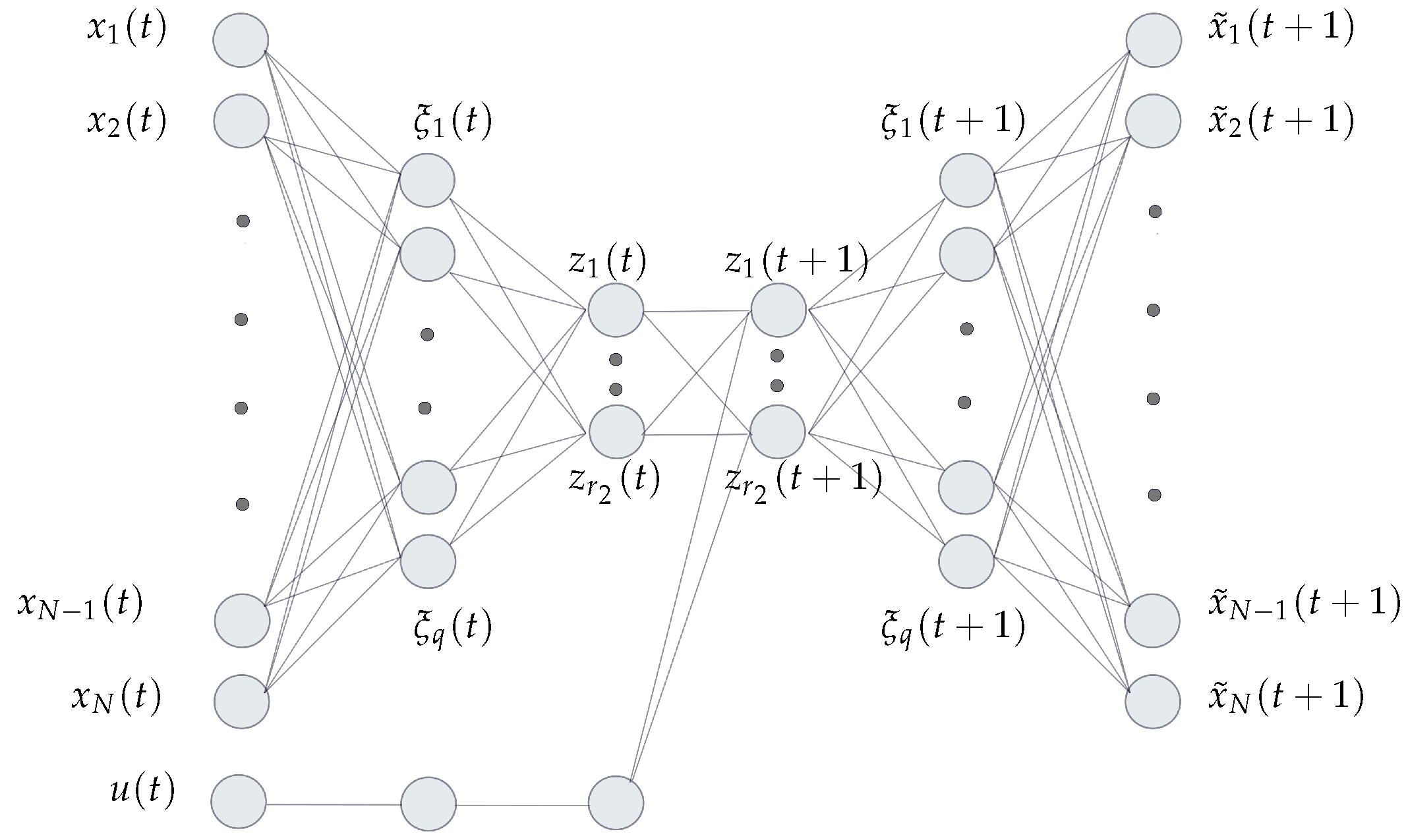
The resulting network-based model order reduction scheme is shown in Figure 4.

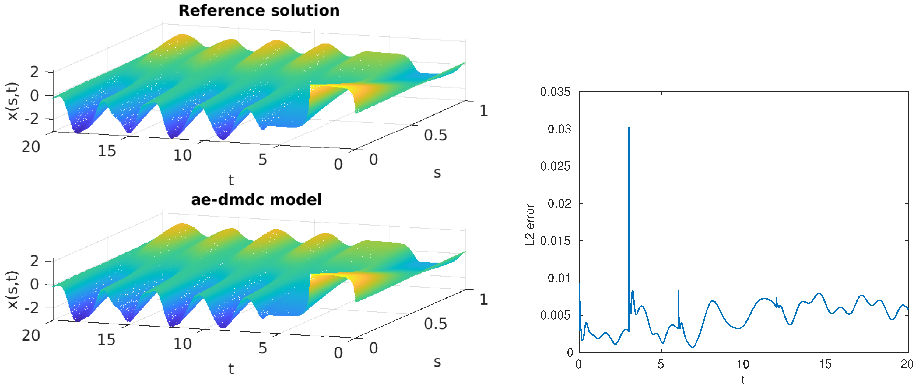
The obtained results with $r_2=17$, $r_1=18$ are shown in Figure 5. On the left of the figure, the comparison of the reference solution and the autoencoder-DMDc (ae-dmdc) based approximation can be seen. On the right part of the figure, the associated approximation error norm is shown.

Next, the identification of a suitable approximation of the output (i.e., measurement) operator is addressed. In terms of the numerical approximation (5) of the pde model (1), the output at time $t\in \mathbb{R}$ is given by

$$\begin{array}{cc}\hfill y\left(t\right)& =x(1,t)\approx {\mathit{c}}^{\mathrm{T}}\mathit{x}\left(t\right)\approx {\mathit{c}}^{\mathrm{T}}{\mathit{\eta }}_2(W_2{U}_{2,r}\mathit{z}\left(t\right)+{\mathit{b}}_2)={\tilde{\mathit{c}}}^{\mathrm{T}}\mathit{z}\left(t\right).\hfill \end{array}$$

For the purpose of providing an optimal minimum squared error approximation of ${\tilde{\mathit{c}}}^{\mathrm{T}}$ the following snapshot matrices have been introduced

$$\begin{array}{c}\hfill Y\hspace{0.17em}=\hspace{0.17em}\left[\begin{array}{ccc}y\left(0\right)& \cdots & y\left(m\right)\end{array}\right],Z\hspace{0.17em}=\hspace{0.17em}\left[\begin{array}{ccc}\mathit{z}\left(0\right)& \cdots & \mathit{z}\left(m\right)\end{array}\right]\hspace{0.17em}=\hspace{0.17em}{U}_{2,r}^{\mathrm{T}}\Xi \end{array}$$

so that with the pseudo–inverse $Z^{†}$ one obtains

$$\begin{array}{c}\hfill Y={\tilde{\mathit{c}}}^{\mathrm{T}}Z,{\tilde{\mathit{c}}}^{\mathrm{T}}=Y{Z}^{†},Z^{†}=Z^{\mathrm{T}}{\left(Z{Z}^{\mathrm{T}}\right)}^{-1}.\end{array}$$

The resulting absolute error of the output approximation is shown in Figure 6 for the two different sensor locations $s_m=1$ and $s_m=0.5$.

It can be seen that a good correspondence is achieved for both sensor locations.

4. Full State Reconstruction Using the Ae-Dmdc Reduced-Order Model

In this section, the reduced-order model with state $\mathit{z}\left(t\right)\in {\mathbb{R}}^{r_2}$ (with $r_2\ll N$) is employed to design algorithms for the reconstruction of the complete state $\mathit{x}\left(t\right)\in {\mathbb{R}}^N$ by combining the available measurement information, the known input $u\left(t\right)$ with the model using two different observer design approaches and the decoder of the previously designed autoencoder. In general, consider an estimate $\widehat{\mathit{z}}$ with the associated full-state estimate $\widehat{\mathit{x}}={\mathit{\eta }}_2(W_2\widehat{\mathit{z}}+{\mathit{b}}_2)$ it holds for the estimation error $\mathit{e}=\widehat{\mathit{x}}-\mathit{x}$ that

$$\begin{array}{c}\hfill \mathit{e}={\mathit{\eta }}_2(W_2\widehat{\mathit{z}}+{\mathit{b}}_2)-\mathit{x}={\mathit{\eta }}_2(W_2\widehat{\mathit{z}}+{\mathit{b}}_2)-{\mathit{\eta }}_2(W_2\mathit{z}+{\mathit{b}}_2)\end{array}$$

so that for a linear decoder mapping ${\mathit{\eta }}_2$ one obtains

$$\begin{array}{c}\hfill \mathit{e}={\mathit{\eta }}_2(W_2(\widehat{\mathit{z}}-\mathit{z})+{\mathit{b}}_2),\end{array}$$

implying that $\mathit{e}\to \mathbf{0}$ if and only if $\widehat{\mathit{z}}-\mathit{z}\to \mathbf{0}$. Thus, providing an estimate in the $\mathit{z}$-coordinates is sufficient for obtaining a reliable estimate in the original coordinates, as long as the autoencoder is adequately trained (i.e., in particular with ${\mathit{\eta }}_2(\mathbf{0}+{\mathit{b}}_2)\approx \mathbf{0}$).

4.1. Reduced-Order Observer

The main idea of the reduced order observer is to prevent redundant estimates and reduce model-dependency of the state estimation scheme [1,2]. For this purpose, the measurements (or parts of them) are directly included unfiltered in the estimator, which is only possible if no significant sensor noise is at place. To introduce the approach, formally consider the state transformation

$$\begin{array}{c}\hfill \mathit{\zeta }=V\mathit{z},V=\left[\begin{array}{c}{\tilde{\mathit{c}}}^{\mathrm{T}}\\ T\end{array}\right]\end{array}$$

with T such that V is invertible, i.e., $rank\left(T\right)=r_2-1$ (as there is only 1 measurement) and $T\mathit{c}=0$, meaning that the rows of T corresponds to basis vectors of the orthogonal complement of the space spanned by the row vector ${\mathit{c}}^{\mathrm{T}}$ (i.e., the measurement subspace). It should be noted that there exist effective numerical algorithms for determining the matrix T, e.g., using null in Matlab.

Next, consider the partition

$$\begin{array}{cc}\hfill \mathit{\zeta }& =\left[\begin{array}{c}{\mathit{\zeta }}_m\\ {\mathit{\zeta }}_r\end{array}\right],\overline{A}=V\tilde{A}{V}^{-1}=\left[\begin{array}{cc}{\overline{A}}_m& {\overline{A}}_{mr}\\ {\overline{A}}_{rm}& {\overline{A}}_r\end{array}\right],\overline{\mathit{b}}=V\tilde{\mathit{b}}=\left[\begin{array}{c}{\overline{\mathit{b}}}_m\\ {\overline{\mathit{b}}}_r\end{array}\right]\hfill \end{array}$$

and the associated reduced order observer

$$\begin{array}{cc}\hfill {\widehat{\mathit{\zeta }}}_r(t+1)& ={\overline{A}}_{rm}y\left(t\right)+{\overline{A}}_r{\widehat{\mathit{\zeta }}}_r\left(t\right)+{\overline{\mathit{b}}}_{r}u\left(t\right)\hfill \end{array}$$

(6a)

$$\begin{array}{cc}\hfill \widehat{\mathit{z}}\left(t\right)& =V^{-1}\left[\begin{array}{c}y\left(t\right)\\ {\widehat{\mathit{\zeta }}}_r\left(t\right)\end{array}\right]\hfill \end{array}$$

(6b)

$$\begin{array}{cc}\hfill \widehat{\mathit{x}}\left(t\right)& ={\mathit{\eta }}_2(W_2\widehat{\mathit{z}}\left(t\right)+{\mathit{b}}_2).\hfill \end{array}$$

(6c)

It is straight forward to verify that the associated observation error $\tilde{\mathit{z}}=\widehat{\mathit{z}}-\mathit{z}$ exponentially converges to zero with time if and only if all eigenvalues of the matrix ${\overline{A}}_r$ are contained in the open unit disk ${\mathbb{U}}_1\subset \mathbb{C}$. If some eigenvalues are contained on the unit circle there are estimation error components (in $\mathit{\zeta }$ coordinates!) that will remain constant but not grow in time, i.e., for small initial errors, small error evolutions can still be achieved. Given that $\mathit{z}=\mathbf{0}$ is mapped onto $\mathit{x}=\mathbf{0}$ the convergence in the original state coordinates can be ensured within some accuracy limitation associated to the approximation performance of the autoencoder.

4.2. Kalman Filter

For comparison purposes, the state estimation by using the Kalman Filter [21,22] is considered. The combination of DMDc models with Kalman Filters has recently been shown to yield quite convincing results [3,17,18,19,20]. One big potential of the Kalman Filter relies on the fact that it provides a minimum estimation error covariance based on a priori statistics of the model and measurement uncertainties, which are considered as white noise processes with covariances $Q\in {\mathbb{R}}^{r_2\times r_2}$ and $r\in \mathbb{R}$ in the present context, i.e.,

$$\begin{array}{cc}\hfill \mathit{z}(t+1)& =\tilde{A}\mathit{z}\left(t\right)+\tilde{\mathit{b}}u\left(t\right)+w\left(t\right),w\left(t\right)\sim \mathcal{N}(\mathbf{0},Q)\hfill \end{array}$$

(7a)

$$\begin{array}{cc}\hfill y\left(t\right)& ={\tilde{\mathit{c}}}^{\mathrm{T}}\mathit{z}\left(t\right)+v\left(t\right),v\left(t\right)\sim \mathcal{N}(0,r).\hfill \end{array}$$

(7b)

Under these assumptions, the minimum estimation error covariance state estimator is given by the following prediction-correction (innovation) scheme (see, e.g., [21])

$$\begin{array}{cc}\hfill & \mathrm{Prediction}\hfill \\ \hfill & {\widehat{\mathit{z}}}_p(t+1)=\tilde{A}\widehat{\mathit{z}}\left(t\right)+\tilde{\mathit{b}}u\left(t\right)\hfill \end{array}$$

(8a)

$$\begin{array}{cc}\hfill & P_p(t+1)=\tilde{A}P\left(t\right){\tilde{A}}^{\mathrm{T}}+Q\hfill \\ \hfill & \mathrm{Kalman}\mathrm{gain}\hfill \end{array}$$

(8b)

$$\begin{array}{cc}\hfill & L(t+1)=P_p(t+1)\tilde{\mathit{c}}({\tilde{\mathit{c}}}^{\mathrm{T}}{P}_p(t+1)\tilde{\mathit{c}}+r)\hfill \\ \hfill & \mathrm{Innovation}\hfill \end{array}$$

(8c)

$$\begin{array}{cc}\hfill & \widehat{\mathit{z}}(t+1)=(I-L(t+1){\mathit{c}}^{\mathrm{T}}){\widehat{\mathit{z}}}_p(t+1)+Ly(t+1)\hfill \end{array}$$

(8d)

$$\begin{array}{cc}\hfill & P(t+1)=(I-L(t+1){\mathit{c}}^{\mathrm{T}})P_p(t+1)\hfill \\ \hfill & \mathrm{Complete}\mathrm{state}\mathrm{reconstruction}\hfill \end{array}$$

(8e)

$$\begin{array}{cc}\hfill & \widehat{\mathit{x}}(t+1)={\mathit{\eta }}_2(W_2\widehat{\mathit{z}}(t+1)+{\mathit{b}}_2)\hfill \end{array}$$

(8f)

with predicted state ${\widehat{\mathit{z}}}_p$, error covariance $P_p$, Kalman (correction) gain L, state estimate $\widehat{\mathit{z}}$ and error covariance P.

Note that the implementation of the Kalman Filter implies the memory usage of a total of $r_2^2+r_2$ floating point variables for storing (and for updating) the error covariance matrix $P\left(t\right)\in {\mathbb{R}}^{r_2\times r_2}$ and the state estimate $\widehat{\mathit{z}}\left(t\right)\in {\mathbb{R}}^{r_2}$. For the case study with $r_2=17$ this yields 306 dynamic variables, while the original pde approximation is based on only 100. On the other hand it should be noticed that the Kalman Filter provides a minimum estimation error covariance, which is in particular useful if one takes into account the stochastic process and measurement noise perturbations. Given the approximative nature of the model (in full-scale with $N=100$ state variables as well as in reduced scale with $r_2=17$ state variables, this uncertainty rejection property can eventually compensate modeling errors up to some point.

4.3. Observer Evaluation

In this section both observer design approaches are compared for two different input scenarios

$$u_1\left(t\right)=\sigma (t-5)-2\sigma (t-10)+\sigma (t-15)$$

(9a)

$$u_2\left(t\right)=cos\left(0.5t\right)\left(\sigma \right(t-5)-2\sigma (t-10)+\sigma (t-15)sin(3t\left)\right)$$

(9b)

giving rise to four different scenarios

(S1)

$u=u_1$ and $s_m=1$, (S2) $u=u_1$ and $s_m=0.5$

(S3)

$u=u_2$ and $s_m=1$, (S4) $u=u_2$ and $s_m=0.5$.

The associated input and state profiles are shown in Figure 7.

For the comparison of the appproaches, the associated approximated evolution of the $L^2$ norm of the observation error profiles is evaluated. Further, to evaluate the associated computational load, the mean computation time per time step $\overline{t}$ and its variance $\nu$ are evaluated for both approaches on a notebook computer with Intel Pentium CPU 4415U with 2.3 GHz.

The results of the evaluation are shown in Figure 8. It can be seen that both observer schemes yield similar estimation performance, with the Kalman Filter performing slightly better in terms of precision for $s_m=1$ and the reduced order observer for $s_m=0.5$. The associated computation times clearly show that the reduced order observer achieves its core calculations about four times as fast as the Kalman Filter, which is due to the higher dimensionality of the Kalman Filter with the required calculation of the covariance matrix.

5. Discussion

As commented above, the implementation of the reduced order observer actually requires only $r_2-1$ (i.e., for the case study with $r_2=17$ this corresponds to only 16) variables, while the Kalman Filter requires the additional information about the error covariance matrix at each time step, yielding a total of $r_2^2+r_2$ variables (i.e., for the case study 306). This implies a significant reduction (by a factor about 19 for the case study) in comparison to the Kalman Filter in terms of memory storage. In addition, as discussed in the previous section, in the performed simulation studies the core calculations of the reduced-order observer were about four times faster than the ones for the Kalman Filter. It should be mentioned anyway, that in the implementation in Matlab, when taking into account the time for the decoding, i.e., the last step in both observer schemes, this time advantage is basically lost and both approaches perform similarly.

As it can be seen, the performance of the Kalman Filter and the reduced order observer are quite comparable for this particular case study. As commented in the introductory discussion for the reduced order observer, this is clearly to be attributed to an output approximation with low noise level. For systems with more sensor noise it is not recommendable to use the unfiltered output directly in the observer scheme.

As a consequence of these results, as long as computation times are below system specific constraints in terms of time scales, both approaches can be employed, while in the case that the computation times should be held as low as possible and that the measurement noise is neglectable, the reduced order observer has clear advantages. This holds true in particular if in addition to the observer scheme some complex calculations or real-time parallel optimizations are performed.

6. Conclusions and Outlook

The combination of autoencoders and dynamic mode decomposition has been employed as a basis for low-dimensional observer design for a class of diffusion-convection-reaction systems using the reduced order observer and Kalman Filter approaches. Using a case study it was shown that both approaches yield satisfactory and comparable results, with the Kalman Filter having a slightly better precision on the cost of significantly higher memory costs, while the reduced order observer provides a comparable performance with very low computational demand and a high degree of simplicity in the design.

Future studies will focus on different, more complex applications, including networks of systems, semilinear pde systems, pdes on higher-dimensional domains (2D, 3D), spatially varying diffusion and convection mechanisms, and study of the impact of the autoencoder structure with more detail (number and size of hidden layers, activation and loss functions, etc.). Comparisons with other model order reduction approaches will be carried out for the respective cases.

References

1. Luenberger, D.G. Observing the state of a linear system. IEEE Trans. Milit. Elect. 1964, 8, 74–80. [Google Scholar] [CrossRef]
2. Luenberger, D.G. An introduction to observers. IEEE Trans. Autom. Control 1971, 16, 596–602. [Google Scholar] [CrossRef]
3. Otto, S.E.; Rowley, C.W. Koopman Operators for Estimation and Control of Dynamical Systems. Annu. Rev. Control Robot. Auton. Syst. 2021, 4, 59–87. [Google Scholar] [CrossRef]
4. Curtain, R.F.; Zwart, H. An Introduction to Infinite-Dimensional Linear Systems Theory; Springer: New York, NY, USA, 1995. [Google Scholar]
5. Krstic, M.; Smyshlyaev, A. Boundary Control of PDEs: A Course on Backstepping Designs; SIAM: Philadelphia, PA, USA, 2008. [Google Scholar]
6. Schaum, A.; Moreno, J.A.; Alvarez, J.; Meurer, T. A simple observer scheme for a class of 1-D semi-linear parabolic distributed parameter systems. In Proceedings of the 2015 European Control Conference, Linz, Austria, 15–17 July 2015; pp. 49–54. [Google Scholar]
7. Schaum, A.; Alvarez, J.; Meurer, T.; Moreno, J.A. State-estimation for a class of tubular reactors using a pointwise innovation scheme. J. Proc. Control 2017, 60, 104–114. [Google Scholar] [CrossRef]
8. Schaum, A. An unknown input observer for a class of diffusion-convection-reaction systems. at-Automatisierungstechnik 2018, 66, 548–557. [Google Scholar] [CrossRef]
9. Schaum, A. Dissipativity in Control Engineering. Applications to Finite and Infinite Dimensional Systems; DeGruyter: Berlin, Germany, 2021. [Google Scholar]
10. Schaum, A.; Koch, S.; Reichhartinger, M.; Meurer, T.; Moreno, J.A.; Horn, M. Nonlinear Observer Design for a 1D Heat Conduction Process. In Proceedings of the 60th IEEE Conference on Decision and Control (CDC), Austin, TX, USA, 13 December 2021. in press. [Google Scholar]
11. Brunton, S.L.; Kutz, J.N. Data-Driven Science and Engineering; Cambridge University Press: Cambridge, UK, 2019. [Google Scholar]
12. Williams, M.O.; Kevrekidis, I.G.; Rowley, C.W. A Data–Driven Approximation of the Koopman Operator: Extending Dynamic Mode Decomposition. J. Nonlinear Sci. 2015, 25, 1307–1346. [Google Scholar] [CrossRef] [Green Version]
13. Proctor, J.L.; Brunton, S.L.; Kutz, J.N. Generalizing Koopman Theory to Allow for Inputs and Control. SIAM J. Appl. Dyn. Syst. 2018, 17, 909–930. [Google Scholar] [CrossRef] [PubMed] [Green Version]
14. Lusch, B.; Kutz, J.N.; Brunton, S.L. Deep learning for universal linear embeddings of nonlinear dynamics. Nat. Commun. 2018, 9, 4950. [Google Scholar] [CrossRef] [PubMed]
15. Maksakov, A.; Palis, S. Koopman-based data-driven control for continuous fluidized bed spray granulation with screen-mill-cycle. J. Process Control 2021, 103, 48–54. [Google Scholar] [CrossRef]
16. Masti, D.; Bemporad, A. Learning nonlinear state–space models using autoencoders. Automatica 2021, 129, 109666. [Google Scholar] [CrossRef]
17. Gomez, D.F.; Lagor, F.D.; Kirk, P.B.; Lind A., H.; Jones, A.R.; Paley, D.A. Data-driven estimation of the unsteady flowfield near an actuated airfoil with embedded pressure sensors. J. Guid. Control Dyn. 2019, 42, 2279. [Google Scholar] [CrossRef]
18. Surana, A. Koopman Operator Based Observer Synthesis for Control-Affine Nonlinear Systems. In Proceedings of the IEEE 55th Conference on Decision and Control (CDC), Las Vegas, NV, USA, 12–14 December 2016; pp. 6492–6499. [Google Scholar]
19. Surana, A.; Banaszuk, A. Linear observer synthesis for nonlinear systems using Koopman Operator framework. IFAC-PapersOnLine 2016, 49, 716–723. [Google Scholar] [CrossRef]
20. Vijayshankar, S.; Nabi, S.; Chakrabarty, A.; Grover, P.; Benosman, M. Dynamic Mode Decomposition and Robust Estimation: Case Study of a 2D Turbulent Boussinesq Flow. In Proceedings of the 2020 American Control Conference, Denver, CO, USA, 1–3 July 2020; pp. 2351–2356. [Google Scholar]
21. Gelb, A. Applied Optimal Estimation; M.I.T. Press: Cambridge, UK, 1978. [Google Scholar]
22. Kalman, R. A New Approach to Linear Filtering and Prediction Problems. Trans. ASME–J. Basic Eng. 1960, 82, 35–45. [Google Scholar] [CrossRef] [Green Version]
23. Alvarez, J.; Lopez, T. Robust dynamic state estimation of nonlinear plants. AIChE J. 1999, 45, 107–123. [Google Scholar] [CrossRef]
24. Aris, R. Introduction to the Analysis of Chemical Reactors; Prentice-Hall: Englewood Cliffs, NJ, USA, 1969. [Google Scholar]
25. Bastin, G.; Dochain, D. On-Line Estimation and Adaptive Control of Bioreactors; Elsevier: Amsterdam, The Netherlands, 1990. [Google Scholar]
26. Dochain, D. State observers for tubular reactors with unknown kinetics. J. Proc. Control 2000, 45, 259–268. [Google Scholar] [CrossRef]
27. Franco-de los Reyes, H.A.; Schaum, A.; Meurer, T.; Alvarez, J. Stabilization of an unstable tubular reactor by nonlinear passive output feedback control. J. Process Control 2020, 93, 83–96. [Google Scholar] [CrossRef]
28. Varma, A.; Aris, R. Stirred pots and empty tubes. In Chemical Reactor Theory; Prentice Hall: Hoboken, NJ, USA, 1977; pp. 79–154. [Google Scholar]
29. Winkin, J.J.; Dochain, D.; Ligarius, P. Dynamical analysis of distributed parameter tubular reactors. Automatica 2000, 36, 349–361. [Google Scholar] [CrossRef]
Figure 1. Solution of the pde model (1) using finite-difference approximation with N = 100 collocation points (top) and corresponding input (bottom).
Algorithms 14 00330 g001
Figure 2. Autoencoder network for empirical basis identification using machine learning.
Algorithms 14 00330 g002
Figure 3. (Left): Comparison of the original data set (top) and the approximated one obtained with the trained autoencoder (bottom). (Right): Approximation error norm.
Algorithms 14 00330 g003
Figure 4. Network-based model-order reduction scheme consisting of an autoencoder network in combination with a linear DMDc-based network.
Algorithms 14 00330 g004
Figure 5. (Left): Comparison of the original solution (top) and the approximated one obtained with the low order ae-dmdc model obtained by combining the trained autoencoder with the DMDc approximation (bottom). (Right): Approximation error norm.
Algorithms 14 00330 g005
Figure 6. Output approximation error for the training data for the two different sensor locations s m .
Algorithms 14 00330 g006
Figure 7. Input scenarios for S1, S2 (left, u = u 1 ) and S3, S4 (right, u = u 2 ).
Algorithms 14 00330 g007
Figure 8. Comparison of the approximated L 2 observation error norm evolutions for the four different scenarios (S1) to (S4) with the respective mean computation times per unit step ( t ¯ r o o , t ¯ k f and the associated variances ν r o o , ν k f obtained in the simulation study.
Algorithms 14 00330 g008
Publisher’s Note: MDPI stays neutral with regard to jurisdictional claims in published maps and institutional affiliations.