Adaptive Refinement in Advection–Diffusion Problems by Anomaly Detection: A Numerical Study

Abstract

We consider advection–diffusion–reaction problems, where the advective or the reactive term is dominating with respect to the diffusive term. The solutions of these problems are characterized by the so-called layers, which represent localized regions where the gradients of the solutions are rather large or are subjected to abrupt changes. In order to improve the accuracy of the computed solution, it is fundamental to locally increase the number of degrees of freedom by limiting the computational costs. Thus, adaptive refinement, by a posteriori error estimators, is employed. The error estimators are then processed by an anomaly detection algorithm in order to identify those regions of the computational domain that should be marked and, hence, refined. The anomaly detection task is performed in an unsupervised fashion and the proposed strategy is tested on typical benchmarks. The present work shows a numerical study that highlights promising results obtained by bridging together standard techniques, i.e., the error estimators, and approaches typical of machine learning and artificial intelligence, such as the anomaly detection task.

1. Introduction

Advection–diffusion problems occur in many applications, such as the simulation of temperature or concentration transport. The numerical solution of this kind of problem has attracted great attention, especially in the case when advection is dominant. Indeed, in this case, standard finite element methods may lead to numerical solutions with nonphysical oscillations, due to a lack of stability. One way to circumvent these difficulties is by adding some artificial diffusion to the discretization. Different stabilization methods have been proposed in the literature; among them, the streamline-upwind Petrov–Galerkin (SUPG) method and streamline-diffusion method (SDM) [1] are probably the most popular ones. In addition, in the numerical solution of stationary linear advection-dominated advection–diffusion problems, two main issues have to be considered. On the one hand, discontinuities in the form of shock-like fronts can occur. Hence, we need a discretization able to approximate these layers on the boundary or in the interior of the domain properly. On the other hand, in order to identify regions where the solution is less regular, it is necessary to have reliable estimates of the accuracy of the computed numerical solution. A priori estimates are often insufficient, since they only yield information on the asymptotic behavior of the error and require regularity assumptions about the solution that are not satisfied in the presence of singularities arising from interior or boundary layers. Thus, a posteriori error estimators should be considered. A posteriori error estimators are computable quantities that provide information about the numerical error, so that they may be used for making judicious mesh modifications. Their computation should be less expensive than the computation of the numerical solution. Moreover, the error estimator should be local and should yield reliable upper and lower bounds for the true error in a user-specified norm. Local lower bounds are necessary to ensure that the grid is correctly refined so that one obtains a numerical solution with a prescribed tolerance using a nearly minimal number of grid points. Indeed, a general approach to approximate the layers properly and reduce the number of unknowns is by using highly non-equidistant meshes instead of equidistant (or uniform) meshes. Starting from some uniform mesh, a numerical solution can be computed; then, by using some information from this, the grid can be adapted with some a posteriori knowledge, thereby obtaining a grid more suited to the problem at hand. This technique is referred to as an adaptive method based on a posteriori error estimation. Adaptive local refinement is therefore an important component for obtaining, in an efficient way, an accurate solution to advection/reaction-dominated problems and has received a great deal of attention in the past three decades; see, for instance, [2,3] for unstructured meshes and [4,5] for structured ones.

A key issue for adaptive refinement is good a posteriori error estimation. For advection–diffusion–reaction equations, one of the initial studies for the comparison of different estimators using the streamline upwind Petrov–Galerkin (SUPG) solution of advection–diffusion–reaction equations was done in [6], and it was shown that none of the estimators was robust with respect to the diffusion coefficient.

In [7], a robust estimator is proposed in the same norm in which the a priori analysis is performed for the SUPG method, namely the SUPG norm. Other examples of estimators obtained using different techniques can be found, for instance, in [8,9,10,11,12].

A final component needed to set up an efficient adaptive scheme is the choice of a proper marking strategy, which allows the selection of the regions to be refined. In theory, the marking strategy should ensure a specific error reduction with respect to the number of refined elements; see [13] and references therein for a review. In practice, most of the time, there are one or more hyper-parameters that need to be correctly tuned. In the present work, we rely on an anomaly detection algorithm that is able to cluster the mesh elements into two sets: the normal and the anomalous ones. In particular, the latter are the elements that will be refined. Anomaly detection usually refers to the task of identifying those behaviors that greatly differ from the standard trend; see [14] for a review. Some recent papers, e.g., [15,16,17], have exploited artificial intelligence techniques based on supervised learning to produce adaptive strategies for the solution of PDEs. In the current work, we adopt an unsupervised technique that does not require any training or any a priori knowledge of the correct mesh elements that should be marked. The anomaly detection task is performed in a completely unsupervised fashion by using the error estimators and the isolation forest algorithm.

The paper is organized as follows: in Section 2, we formulate the problem and we recall the main features of the adopted error estimators and the anomaly detection algorithms. In Section 3, we report several examples, which confirm the good performance of the proposed strategy. Finally, in Section 4, we discuss some possible future work.

2. Problem Formulation

We consider scalar advection–diffusion–reaction problems that, in general, can be modeled as:

$$\left\{\begin{array}{ccc}-div(\epsilon \nabla u)+\mathbf{b}·\nabla u+\alpha u=f\hfill & \mathrm{in}\Omega \hfill & \\ u=u_D\hfill & \mathrm{on}{\Gamma }_D\hfill & \\ {\displaystyle \epsilon \frac{\partial u}{\partial n}=g}\hfill & \mathrm{on}{\Gamma }_N,\hfill \end{array}\right.$$

(1)

where $\Omega$ in ${\mathbb{R}}^2$ is a Lipschitz domain with a polygonal boundary $\Gamma$. In particular, $\Gamma$ consists of two non-overlapping components ${\Gamma }_D$ e ${\Gamma }_N$, such that $\Gamma ={\overline{\Gamma }}_D\cup {\overline{\Gamma }}_N$ and ${\Gamma }_D\cap {\Gamma }_N=\varnothing$. In Equation (1), the function u is the unknown, while $\epsilon$ is the diffusivity coefficient, $\mathbf{b}=[b_1,b_2]$ is the advective field with $\nabla ·\mathbf{b}=0$, $\alpha \ge 0$ a.e. in $\Omega$ is the reaction coefficient, f is the source and $\mathbf{n}$ is the unit outward normal vector. We will also assume the following:

(A1)

$0<\epsilon \ll 1$.

(A2)

$\mathbf{b}\in W^{1,\infty }{(\Omega )}^2$, $\alpha \in L^{\infty }(\Omega )$, $f\in L^2(\Omega )$ and $g\in L^2\left({\Gamma }_N\right)$.

(A3)

There exist two constants, $\beta \ge 0$ and $c_b\ge 0$, independent of $\epsilon$, such that

${\displaystyle -\frac{1}{2}div\mathbf{b}+\alpha }$${\displaystyle \ge \beta }$ and ${\Vert \alpha \Vert }_{L^{\infty }}\le c_b\beta$.

As already mentioned in the Introduction, scalar advection–diffusion equations describe the transport of scalar quantities, such as temperature or concentration. This transport term is composed of a diffusive part and an advective part.

From the mathematical proprieties of these two components, it is possible to distinguish regular or exponential layers, parabolic layers and internal or boundary layers. The accurate computation of these singularity regions is crucial to obtain a reliable approximation of the numerical solution of advection–diffusion problems. Standard finite element methods may lead to numerical solutions with nonphysical oscillations, due to the lack of stability of the considered method. (Here, stability is not meant in the sense of the continuous dependence of the solution on the initial data, but rather in the sense of reducing the oscillations occurring in the numerical solution).

Setting

$$V:=H_D^1(\Omega )=\{\phi \in H^1(\Omega ):\phi =0 \mathrm{on} {\Gamma }_D\},$$

(2)

the weak formulation of problem (1) is:

$$\mathrm{Find}u\in V:a(u,v)=\ell \left(v\right)\forall v\in V,$$

(3)

where we introduced the bilinear form $a:V\times V\to \mathbb{R}$

$$a(u,v)={\int }_{\Omega }\epsilon \nabla u·\nabla vd\Omega +{\int }_{\Omega }v\mathbf{b}·\nabla ud\Omega +{\int }_{\Omega }\alpha uvd\Omega$$

(4)

and the functional $\ell :V\to \mathbb{R}$:

$$\ell \left(v\right)={\int }_{\Omega }fvd\Omega +{\int }_{{\Gamma }_N}gvd\gamma .$$

(5)

Let ${\left\{{\mathcal{T}}_h\right\}}_h$ be a family of conforming triangulations of $\overline{\Omega }$ into triangles T with diameter $h_T\le h$, with ${\displaystyle h=\underset{T\in {\mathcal{T}}_h}{max}{h}_T}$. Let ${\mathbb{P}}_m$ be the space of polynomials of degree at most m, and we set

$$V_h:=\left\{\varphi \in C\left(\overline{\Omega }\right){\left|\varphi \right|}_T\in {\mathbb{P}}_m\forall T\in {\mathcal{T}}_h,\varphi =0 \mathrm{on} {\Gamma }_D\right\}.$$

By projecting in the space $V_h\subset V$ of continuous piecewise linear finite elements and stabilizing with the SUPG method [1], we can write the generalized formulation:

$$\mathrm{Find}{u}_h\in V_h:a_h(u_h,v_h)={\ell }_h\left(v_h\right)\forall v_h\in V_h,$$

(6)

where

$$a_h(u_h,v_h)=a(u_h,v_h)+b_h(u_h,v_h)\mathrm{and} {\ell }_h\left(v_h\right)=\ell \left(v_h\right)+m_h\left(v_h\right).$$

The terms $b_h(u_h,v_h)$ and $m_h\left(v_h\right)$ are the stabilizing terms and they are necessary to reduce the possible numerical oscillations due to the classical Galerkin formulation.

2.1. Mesh Adaptation

We are interested in those applications where the diffusive term ${\displaystyle -div(ϵ\nabla u)}$ is dominated either by the convective term ${\displaystyle \mathbf{b}·\nabla u}$ or by the reaction term ${\displaystyle \alpha u}$. In such cases, the solution may exhibit some boundary layers that arise from strong gradient variations. Since the presence of abrupt changes in the behavior of the solution is usually localized to certain regions, it is meaningful to adopt adaptive strategies in order to increase the number of degrees of freedom in those local regions only. This allows us to have more control and hence better final accuracy is reached in the approximation of the solution. In practice, the adaptivity of the mesh is obtained by adopting a posteriori error estimators. In the present work, we decided to compare the performance of three error estimators considered in their basic formulation; see [18]. In fact, according to the type of problem at hand, more advanced and specific versions of each of the considered error estimator can be developed. In our case, we decided to design a strategy that would make equivalent the different behaviors that are usually observed when different marking strategies are adopted, or when different problem settings are considered. For the sake of clarity, we recall the main features of the adopted error estimators.

2.1.1. Residual Error Estimator

The first error estimator considered is the residual type ${\eta }_R$, defined as:

$${\eta }_{R,T}:={\left\{h_T^2{∥Re{s}_T∥}_{L^2\left(T\right)}^2+\sum _{E\subset \partial T}{h}_E{∥Re{s}_E∥}_{L^2\left(E\right)}^2\right\}}^{1/2},$$

(7)

where we denote by $Re{s}_T$ and $Re{s}_E$ the residual computed on each triangle T and on each edge E, respectively. Meanwhile, $h_T$ and $h_E$ refer to the diameter of the triangle T and to the length of the edge E in the triangle T. The usual definitions for $Re{s}_T$ and $Re{s}_E$ are adopted:

$$Re{s}_T\left(u_h\right)=f+\epsilon \Delta u_h-\mathbf{b}·\nabla u_h-\alpha u_h,$$

$$Re{s}_E\left(u_h\right)=\left\{\begin{array}{ccc}{[{\mathbf{n}}_E·\epsilon \nabla u_h]}_E& \mathrm{if} E \mathrm{in} \Omega & \\ (g-{\mathbf{n}}_E·\epsilon \nabla u_h)& \mathrm{if} E \mathrm{on} {\Gamma }_N& \\ 0& \mathrm{if} E \mathrm{on} {\Gamma }_D,\end{array}\right.$$

where ${\mathbf{n}}_E$ denotes the unit normal vector to the edge E and the symbol ${[·]}_E$ denotes the jump of a function across the interface E.

2.1.2. A Zienkiewicz–Zhu Type Error Estimator

This type of error estimator is based on reconstructing the gradient of the original solution by a simple averaging technique. In particular, it is defined as:

$${\eta }_{Z,T}:={\parallel G\left(u_h\right)-\nabla u_h\parallel }_{L^2\left(T\right)}.$$

(8)

In our case, the function $G\left(u_h\right)$ is constructed by evaluating the function $\nabla u_h$ on the barycenter of each triangle and then by averaging across those triangles that share a common vertex.

2.1.3. Error Estimator Based on the Solution of Auxiliary Local Problems

As the last error estimator, we consider an error estimator constructed by solving auxiliary local Neumann problems:

$${\eta }_{N,T}:=\parallel |v_T{|\parallel }_T,$$

(9)

where the symbol $\parallel |·|\parallel$ denotes the energy norm and $v_T$ is a function belonging to the set $V_T$,

$$V_T:=span\left\{b_T,b_E:E\in \mathbb{E}\left(T\right)\backslash {\mathbb{E}}_{h,D}\right\},$$

(10)

which approximates the solution of the following auxiliary problem:

$$\left\{\begin{array}{ccc}-\epsilon \Delta u_T+\mathbf{b}·\nabla u_T+\alpha u_T=Re{s}_T\left(u_h\right)\hfill & \mathrm{in}& T\hfill \\ {\displaystyle \epsilon \frac{\partial u_T}{\partial {\mathbf{n}}_T}=Re{s}_E\left(u_h\right)}\hfill & \mathrm{on}& \partial K\backslash {\Gamma }_D\hfill \\ u_T=0\hfill & \mathrm{on}& \partial T\cap {\Gamma }_D.\hfill \end{array}\right.$$

(11)

Note that, in definition (10), we use the bubble functions related to the triangle T and to the edge E; see [19] for additional details.

The mesh refinement and the computation of the finite element approximate solution were performed by using the software FreeFem ++, version 3.5 [20]. In particular, the software makes available an automatic mesh generator, based on the Delaunay–Voronoi algorithm [21], and a metric-based anisotropic mesh adaptation function [22].

2.2. Anomaly Detection

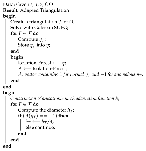
The term anomaly detection is used in the context of time-series or Big Data whenever there are outliers or anomalous points to be identified. In particular, points that follow a standard trend or can be observed to have expected behavior are labeled as normal; otherwise, they become anomalous. In the present work, we use the Isolation Forest (IF) algorithm [23,24], which refers to an unsupervised technique developed to detect anomalies in the considered dataset. In order to isolate the points that deviate from the expected trend, the IF constructs a forest of binary trees by randomly selecting a feature and then randomly selecting a split value. The resulting number of required splittings is equivalent to the path length from the root node to the terminating node. Anomalies usually produce rather shorter paths compared to normal points. IF has a linear time complexity and it does not need any labeled data; hence, it works in a completely unsupervised fashion. In the present work, we use the implementation provided by the Python library scikit-learn [25]. In order to control the randomness, and hence to make the experiments reproducible, we set the parameter random_state = 0. All the other parameters are used with the default settings. The algorithm that we propose employs any error estimator described in the previous subsection in order to acquire an estimate of the error function, localized at every triangle. Then, the IF takes as input an array of values containing the error estimator for each triangle. The anomalies are those values where the estimated error is rather large. Therefore, the anomalous values correspond to those triangles that should be refined. In order to improve the performance of the adopted error estimator, we also ran some benchmarks by setting the contamination parameter $c=0.3$. The contamination acts as a cutoff on the returned values. In particular, $c=0.3$ means that only the top $30\%$ negative scores are labeled as anomalies. The set-up for c was experimentally derived and was in line with the fact that the boundary layers are usually confined to specific regions; hence, usually, there is no need to refine large areas of the computational domain. In certain cases, the use of $c=0.3$ helped to achieve a final refinement even more localized to the problematic areas and, thus, the performance of the three error estimators became equivalent in terms of the reached accuracy per number of refinements. An outline of the proposed algorithm is presented in Algorithm 1.

Algorithm 1: Pseudo-code for the proposed algorithm.

3. Numerical Results

In this section, we show the numerical results on four different benchmarks. Since the exact solution is always unknown, we estimated the $L^2$ norm and the $H^1$ seminorm of the error $e:=u_{ex}-u_h$, by computing $u_{ex}$ with a very fine triangular mesh. In this case, the initial mesh is globally and uniformly refined for several levels. Global uniform refinement prevents an accurate representation of the solution from being reached; hence, we stopped the adaptive refinement procedure when the error values became stagnant or oscillating around a certain threshold. In order to increase the stability of the computation of the solution $u_{ex}$, we improved the used quadrature formula in the evaluation of the integrals for the Galerkin method by setting the parameter qft = qf7pT or by using qft = qf9pT, which are Gaussian quadrature rules of order 8 and 10, respectively; see, e.g., [26], available with the FreeFem integration routines. In general, when the order increases, the Gaussian rule may become unstable; moreover, due to the triangular domains, suitable rules should be constructed; see, e.g, [27,28,29] and references therein. In our tests, we could obtain more stable results for the computation of the $L^2$ norm but, for the $H^1$ seminorm, we could still observe some divergent cases. For every example, we compared the achieved results with the global uniform refinement strategy, in terms of accuracy and in terms of the order of convergence. In order to obtain the appropriate error reduction, the produced mesh should satisfy certain optimality requirements; see, for example, [13,30]. Since this aim goes beyond the scope of the current paper, we only conducted the following experiments by using the anisotropic mesh adaptation function provided by the FreeFem library.

3.1. Example 1: A Reaction–Diffusion Problem

The first example is a reaction–diffusion problem ([31]), where the velocity field $\mathbf{b}$ is zero. In this case, the computational domain is the unit square, $\Omega =[0,1]\times [0,1]$, the source $f=0$, $\epsilon ={10}^{-3}$ e $\alpha =1$. The boundary conditions are shown in Figure 1, while an approximation of the solution is shown in Figure 2.

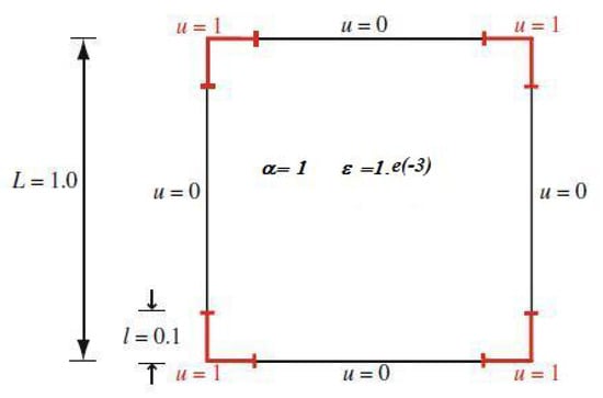
Figure 1. Boundary conditions of example 1.

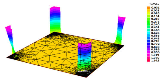
Figure 2. Computed solution for example 1, displayed on the mesh adapted with ${\eta }_Z$ and c = 0.3.

Since homogeneous boundary conditions are assigned, besides at the four corners, we expect the solution to be zero almost everywhere except at the corners where it spikes to one. In Figure 3, on the left, we report the adapted mesh by using the residual error estimator. The four corners are highly refined, but we can also observe a rather dense grid in the middle of $\Omega$, which seems unnecessary for this example. Therefore, we applied a threshold to the percentage of values that should be considered anomalous. By trying several different values, we experimentally derived that a good setting for the contamination parameter in the IF algorithm was 0.3. In these terms, only the points with the top $30\%$ negative values will be considered anomalous. With this strategy, we can localize even more by neglecting a certain percentage of triangles that would otherwise be marked as anomalous. The obtained result with this setting can be seen in Figure 3, right. In Table 1, we report the estimated error in the $L^2$ norm and in $H^1$ seminorm, together with the number of elements (NT) per level of refinement (n), in both cases, i.e., c = auto and c = 0.3. The improvement with the second strategy is evident especially at the final stage: with the same order of magnitude of employed elements, one order of accuracy is gained in the $L^2$ norm. Finally, in Figure 4, we show the comparison with global refinement.

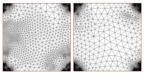
Figure 3. Adapted meshes for example 1 by using the residual-based error estimator. (Left) The last performed step, where the mesh is mostly refined at the four corners. (Right) The final mesh obtained with c = 0.3; the corners are highly refined with respect to the rest of the domain.

Table 1. $L^2$ norm and $H^1$ seminorm of the error for example 1. The residual-based error estimator was employed.

c = auto				c = 0.3
$n$	NT	$L^2$	$H^1$	NT	$L^2$	$H^1$
0	112	1.3 × 10${}^{-2}$	2.0 × 10${}^{-2}$	-	-	-
1	439	1.0 × 10${}^{-2}$	4.3 × 10${}^{-2}$	382	1.1 × 10${}^{-2}$	5.1 × 10${}^{-3}$
2	1388	6.2 × 10${}^{-3}$	1.6 × 10${}^{-3}$	1598	4.8 × 10${}^{-3}$	2.3 × 10${}^{-3}$
3	3882	2.3 × 10${}^{-3}$	1.8 × 10${}^{-3}$	5860	1.2 × 10${}^{-3}$	6.9 × 10${}^{-4}$
4	8860	1.2 × 10${}^{-3}$	2.2 × 10${}^{-4}$	8995	7.5 × 10${}^{-4}$	2.0 × 10${}^{-4}$

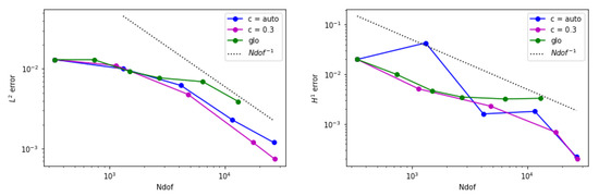
Figure 4. Error behavior for example 1 when ${\eta }_R$ is adopted. (Left) The estimated $L^2$ norm of the error is displayed. (Right) The estimated $H^1$ seminorm of the error is shown.

In Figure 5, we show the results obtained by using the gradient recovery-based error estimator ${\eta }_Z$. Moreover, in this case, we performed two tests: one with c = auto and one with c = 0.3. Table 2 collects the $L^2$ norm error and $H^1$ seminorm error. In this case, the benefit of introducing the cutoff percentile is less evident than in the previous example, but we notice that by reducing the number of elements at the first level, more elements were marked at the successive levels compared with the standard case (i.e., c = auto). This behavior did not lead to a significant gain in accuracy, but the resulting mesh appears more suitable to handle this example since the refinement is more localized at the four corners. In Figure 6, we show the comparison with global refinement. Finally, in Figure 7, the results obtained with ${\eta }_N$ and with c = auto (on the left) and c = 0.3 (on the right) are shown. In Table 3, we report the results for the $L^2$ norm and $H^1$ seminorm estimates. The resulting mesh, adapted with c = 0.3, does not improve the reached accuracy compared to the case c = auto. In fact, the refinement, besides appearing not to be symmetric, appears to be less localized. This can happen as the contamination parameter is only useful to select the top $30\%$ of anomalous triangles, which are not necessarily the ones that exhibit the largest error among the anomalies. In Figure 8, we show the comparison with global refinement. In all three cases, the adaptive refinement achieved better accuracy and a better order of convergence compared to global refinement per used degrees of freedom.

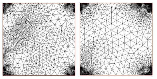
Figure 5. Adapted meshes for example 1 with the gradient recovery-based error estimator. (Left) The adapted mesh at the very last step and parameter c = auto. (Right) The mesh obtained at the last step with the estimator ${\eta }_Z$ and c = 0.3.

Table 2. $L^2$ and $H^1$ error for example 1 by using the gradient recovery error estimator.

c = auto				c = 0.3
$n$	NT	$L^2$	$H^1$	NT	$L^2$	$H^1$
0	112	1.3 × 10${}^{-2}$	2.0 × 10${}^{-2}$	-	-	-
1	523	1.0 × 10${}^{-2}$	4.5 × 10${}^{-2}$	402	1.1 × 10${}^{-2}$	6.3 × 10${}^{-3}$
2	1727	5.1 × 10${}^{-3}$	3.1 × 10${}^{-3}$	1729	5.2 × 10${}^{-3}$	7.8 × 10${}^{-4}$
3	3567	1.0 × 10${}^{-3}$	1.3 × 10${}^{-3}$	6631	1.3 × 10${}^{-3}$	5.2 × 10${}^{-4}$
4	8065	7.8 × 10${}^{-4}$	3.8 × 10${}^{-4}$	10,053	8.1 × 10${}^{-4}$	1.2 × 10${}^{-4}$

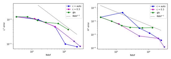
Figure 6. Error behavior for example 1 when ${\eta }_Z$ is adopted. (Left) The estimated $L^2$ norm of the error is displayed. (Right) The estimated $H^1$ seminorm is shown.

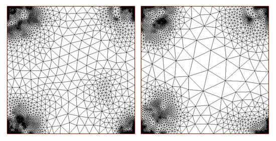
Figure 7. Resulting meshes for example 1 and ${\eta }_N$ error estimator. (Left) The final mesh obtained by setting c = auto. (Right) The final mesh obtained by setting c = 0.3.

Table 3. $L^2$ and $H^1$ error for example 1 by using the ${\eta }_N$ error estimator.

c = auto				c = 0.3
$n$	NT	$L^2$	$H^1$	NT	$L^2$	$H^1$
0	112	1.3 × 10${}^{-2}$	2.0 × 10${}^{-2}$	-	-	-
1	421	1.1 × 10${}^{-2}$	6.0 × 10${}^{-3}$	421	1.1 × 10${}^{-2}$	6.0 × 10${}^{-3}$
2	2171	4.8 × 10${}^{-3}$	6.3 × 10${}^{-3}$	1566	5.1 × 10${}^{-3}$	4.7 × 10${}^{-3}$
3	7170	1.5 × 10${}^{-3}$	4.8 × 10${}^{-4}$	5754	2.9 × 10${}^{-3}$	1.3 × 10${}^{-3}$
4	12,106	8.9 × 10${}^{-4}$	4.0 × 10${}^{-4}$	8574	1.9 × 10${}^{-3}$	1.4 × 10${}^{-3}$

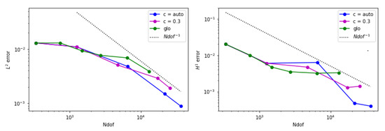
Figure 8. Error behavior for example 1 when ${\eta }_N$ is adopted. (Left) The estimated $L^2$ norm of the error is displayed. (Right) The estimated $H^1$ seminorm is shown.

3.2. Example 2: The Channel Test

We report the second benchmark presented in [32], “the channel test”, which is an advection-dominant problem. The domain $\Omega$ is chosen to be L-shaped: $\Omega ={[0,4]}^2{\backslash [0,2]}^2$. The data of the problem are $\epsilon ={10}^{-3},f=0,\alpha =0,\mathbf{b}=[y,-x]$, while the boundary conditions are shown in Figure 9.

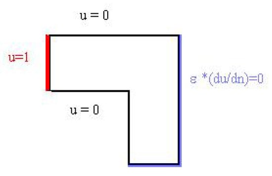
Figure 9. Boundary conditions for example 2.

In Figure 10, on the left, we show the final stage of the adapted mesh according to the residual-based error estimator, while, on the right, we show a 3D plot of the computed solution on the final mesh. The error estimates for the $L^2$ norm and $H^1$ seminorm are reported in Table 4.

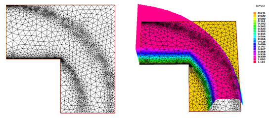
Figure 10. Adapted meshes for example 2 and residual-based error estimator. (Left) The mesh at the final stage. (Right) A 3D plot of the computed solution with the final mesh.

Table 4. Error in $L^2$ norm and $H^1$ seminorm for example 2 obtained with the residual-based error estimator.

n	NT	${\mathit{L}}^2$	${\mathit{H}}^1$
0	1282	2.7 × 10${}^{-1}$	7.8 × 10${}^{-1}$
1	1319	1.7 × 10${}^{-1}$	4.7 × 10${}^{-1}$
2	1531	1.1 × 10${}^{-1}$	1.6 × 10${}^{-1}$
3	1908	8.4 × 10${}^{-2}$	7.1 × 10${}^{-2}$
4	2227	7.8 × 10${}^{-2}$	9.0 × 10${}^{-2}$
5	2597	6.0 × 10${}^{-2}$	4.7 × 10${}^{-2}$
6	3303	4.9 × 10${}^{-2}$	3.8 × 10${}^{-2}$
7	4246	4.6 × 10${}^{-2}$	3.2 × 10${}^{-2}$
8	5111	4.4 × 10${}^{-2}$	2.7 × 10${}^{-2}$
9	6584	4.1 × 10${}^{-2}$	1.3 × 10${}^{-2}$
10	7737	4.1 × 10${}^{-2}$	1.2 × 10${}^{-2}$
11	8844	4.1 × 10${}^{-2}$	1.2 × 10${}^{-2}$

The ${\eta }_R$ and the anomaly detection strategy in this case led to the refinement of very few elements at each step. At the end, the two circular layers and the boundary layer near the non-convex angle were correctly identified and refined. The error e in both $L^2$ norm and $H^1$ seminorm steadily decreased. In this case, using $c=0.3$ appeared meaningless as few elements were refined at each level. In Figure 11, we show the comparison between the adaptive refinement obtained by using ${\eta }_R$ and the global refinement strategy. The adaptive refinement at certain levels decreases with a superlinear order of convergence in the $L^2$ norm. Meanwhile, on the $H^1$ seminorm, the behavior is not monotonic but we can still observe convergence, with better final accuracy compared to the global refinement approach.

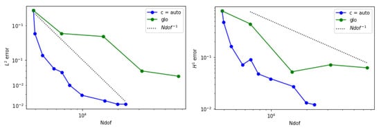
Figure 11. Error behavior for example 2 when ${\eta }_R$ is adopted. (Left) The estimated $L^2$ norm of the error is displayed. (Right) The estimated $H^1$ seminorm is shown.

The resulting mesh obtained by using the gradient recovery error estimator and the ${\eta }_N$ error estimator are shown in Figure 12, and in Table 5 and Table 6, we report the error estimates.

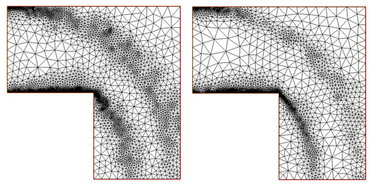
Figure 12. Adapted meshes. (Left) The mesh obtained at the last level by using the ${\eta }_N$ error estimator. (Right) The final stage of the adapted mesh by using the gradient-based error estimator.

Table 5. Error in $L^2$ norm and $H^1$ seminorm for example 2 obtained with the gradient recovery error estimator.

n	NT	${\mathit{L}}^2$	${\mathit{H}}^1$
0	1282	2.7 × 10${}^{-1}$	7.8 × 10${}^{-1}$
1	2296	1.1 × 10${}^{-1}$	1.7 × 10${}^{-1}$
2	5538	6.1 × 10${}^{-2}$	8.2 × 10${}^{-2}$
3	8243	4.9 × 10${}^{-2}$	4.0 × 10${}^{-2}$
4	11,957	4.5 × 10${}^{-2}$	3.0 × 10${}^{-2}$
5	16,894	4.4 × 10${}^{-2}$	2.2 × 10${}^{-2}$

Table 6. Error in $L^2$ norm and $H^1$ seminorm for example 2 obtained with the “Neumann auxiliary” error estimator.

n	NT	${\mathit{L}}^2$	${\mathit{H}}^1$
0	1282	2.7 × 10${}^{-1}$	7.8 × 10${}^{-1}$
1	2348	1.1 × 10${}^{-1}$	2.0 × 10${}^{-1}$
2	6488	4.8 × 10${}^{-2}$	5.2 × 10${}^{-2}$
3	16,533	4.3 × 10${}^{-2}$	1.1 × 10${}^{-2}$
4	16,726	4.2 × 10${}^{-2}$	9.3 × 10${}^{-3}$

We note that, for this example, the adaptive refinement was interrupted when the error became stagnant and, hence, by looking at the reached accuracy, the three error estimators seem rather equivalent. Looking at the resulting adapted meshes, the one obtained with ${\eta }_Z$ is the less refined at the larger circular inner layer. Regarding the boundary layer on the short edge of the L-domain and the smaller circular layer, ${\eta }_R,{\eta }_Z$ and ${\eta }_N$ provided good error estimation for the IF algorithm to correctly label the anomalous triangles. Finally, in Figure 13 and Figure 14, we show the comparisons with the global refinement. Moreover, in this case, the adapted meshes were better than the uniform globally refined mesh, as we could observe a greater decrease in the error and hence better final accuracy per used degrees of freedom.

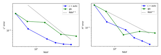
Figure 13. Error behavior for example 2 when ${\eta }_Z$ is adopted. (Left) The estimated $L^2$ norm of the error is displayed. (Right) The estimated $H^1$ seminorm is shown.

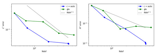
Figure 14. Error behavior for example 2 when ${\eta }_N$ is adopted. (Left) The estimated $L^2$ norm of the error is displayed. (Right) The estimated $H^1$ seminorm is shown.

3.3. Example 3: The Pinched Domain

In this example, we consider a disk with a hole. The boundary of the domain consists of two disconnected components: ${\Gamma }_1:=\{x=cos\left(t\right);y=sin\left(t\right);t\in [0,2\pi ]\}$ is the outer boundary, while ${\Gamma }_2:=\{x=0.3+0.3cos\left(t\right);y=0.3sin\left(t\right);t\in [0,2\pi ]\}$ is the boundary of the inner hole. The input data are: $\epsilon ={10}^{-10}$, $f=0$, $\alpha =1$, $\mathbf{b}=[2,1]$. We apply discontinuous Dirichlet boundary conditions: $u=0$ on ${\Gamma }_1$ and $u=1$ on ${\Gamma }_2$. Therefore, we expect the rise of the two inner layers. The results for the adapted meshes with the three error estimators are shown in Figure 15, Figure 16 and Figure 17. In Table 7, Table 8 and Table 9, we report the error estimates in the $L^2$ norm and $H^1$ seminorm.

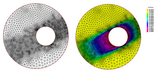
Figure 15. Results for example 3 with ${\eta }_R$. (Left) The final adapted mesh. (Right) The final adapted mesh with the projected isolines of the computed solution.

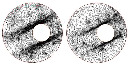
Figure 16. Results for example 3 with ${\eta }_Z$ error estimator. (Left) The last obtained mesh by using c = auto. (Right) The refined mesh at the last performed step with c = 0.3.

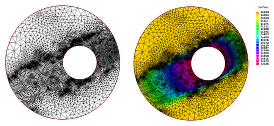
Figure 17. Results for example 3 with ${\eta }_N$. (Left) The resulting adapted mesh. (Right) The resulting adapted mesh with the isolines projection of the computed solution.

Table 7. Error in $L^2$ norm and $H^1$ seminorm for example 3 obtained with the residual-based error estimator.

n	NT	${\mathit{L}}^2$	${\mathit{H}}^1$
0	672	1.1 × 10${}^{-1}$	6.8 × 10${}^{-3}$
1	1603	1.0 × 10${}^{-1}$	3.5 × 10${}^{-3}$
2	2042	9.2 × 10${}^{-2}$	3.0 × 10${}^{-3}$
3	3396	7.6 × 10${}^{-2}$	2.7 × 10${}^{-3}$
4	6004	4.5 × 10${}^{-3}$	2.2 × 10${}^{-3}$
5	8006	3.9 × 10${}^{-3}$	1.5 × 10${}^{-3}$

Table 8. Error in $L^2$ norm and $H^1$ seminorm for example 3 obtained with the gradient recovery error estimator.

c = auto				c = 0.3
$n$	NT	$L^2$	$H^1$	NT	$L^2$	$H^1$
0	672	1.1 × 10${}^{-1}$	6.8 × 10${}^{-3}$	-	-	-
1	1356	8.7 × 10${}^{-2}$	3.0 × 10${}^{-3}$	865	1.1 × 10${}^{-1}$	1.3 × 10${}^{-3}$
2	3888	5.6 × 10${}^{-2}$	1.6 × 10${}^{-3}$	2897	5.9 × 10${}^{-2}$	2.0 × 10${}^{-3}$
3	9569	1.1 × 10${}^{-2}$	1.5 × 10${}^{-3}$	4418	2.9 × 10${}^{-2}$	1.9 × 10${}^{-3}$
4	17,663	2.0 × 10${}^{-2}$	1.1 × 10${}^{-3}$	6507	1.9 × 10${}^{-2}$	1.8 × 10${}^{-3}$
5				9442	1.7 × 10${}^{-2}$	1.2 × 10${}^{-3}$

Table 9. Error in $L^2$ norm and $H^1$ seminorm for example 3 obtained with ${\eta }_N$ error estimator.

c = auto				c = 0.3
$n$	NT	$L^2$	$H^1$	NT	$L^2$	$H^1$
0	672	1.1 × 10${}^{-1}$	6.8 × 10${}^{-3}$	-	-	-
1	2000	9.2 × 10${}^{-2}$	2.7 × 10${}^{-3}$	1964	8.9 × 10${}^{-2}$	2.2 × 10${}^{-3}$
2	2802	7.2 × 10${}^{-2}$	3.8 × 10${}^{-3}$	2959	6.6 × 10${}^{-2}$	1.6 × 10${}^{-3}$
3	4866	5.4 × 10${}^{-2}$	3.9 × 10${}^{-3}$	4027	5.6 × 10${}^{-2}$	6.1 × 10${}^{-4}$
4	11,156	1.8 × 10${}^{-2}$	1.9 × 10${}^{-3}$	5910	4.5 × 10${}^{-2}$	3.0 × 10${}^{-4}$
5	17,658	1.7 × 10${}^{-3}$	1.4 × 10${}^{-3}$	8570	3.0 × 10${}^{-2}$	3.0 × 10${}^{-4}$
6				12,302	1.4 × 10${}^{-2}$	3.0 × 10${}^{-4}$

For this example, the poorest performance is obtained by the ${\eta }_Z$ error estimator. Indeed, the final mesh displayed in Figure 16, on the left, shows an over-refinement spread along two narrow stripes across the whole domain $\Omega$. This seems unnecessary as the main change should happen around the boundary ${\Gamma }_2$; hence, we produced another mesh—see Figure 16 on the right—to limit the number of triangles that would be refined. The use of $c=0.3$ did not produce any significant change when ${\eta }_R$ was employed, while, when ${\eta }_N$ was adopted, we could appreciate a drastic reduction in the refined number of elements at every level, which did not affect the reached accuracy.

In Figure 18, Figure 19 and Figure 20, we report the comparison with the global refinement strategy. Regarding the use of ${\eta }_R$ and the contamination parameter c = 0.3, the performance becomes worse, as it becomes comparable to global refinement. Concerning the ${\eta }_Z$ error estimator, although the error reduction is still better than global refinement in the $L^2$ norm, we can observe a rather uniform behavior when it comes to the $H^1$ seminorm. Regarding the ${\eta }_N$, the achieved results are better than global refinement for the $L^2$ norm, while, in the $H^1$ seminorm, the use of the contamination parameter yields a relevant reduction in the error per used degrees of freedom.

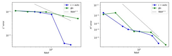
Figure 18. Error behavior for example 3 when ${\eta }_R$ is adopted. (Left) The estimated $L^2$ norm of the error is displayed. (Right) The estimated $H^1$ seminorm is shown.

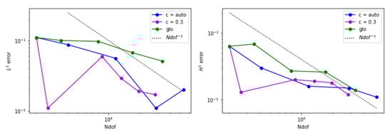
Figure 19. Error behavior for example 3 when ${\eta }_Z$ is adopted. (Left) The estimated $L^2$ norm of the error is displayed. (Right) The estimated $H^1$ seminorm is shown.

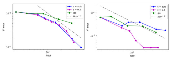
Figure 20. Error behavior for example 3 when ${\eta }_N$ is adopted. (Left) The estimated $L^2$ norm of the error is displayed. (Right) The estimated $H^1$ seminorm is shown.

3.4. Example 4: Parabolic and Exponential Boundary Layers

As the last example, we consider the problem reported in [6]. The computational domain $\Omega$ is the unit square. The input data are $\epsilon ={10}^{-6}$, $\mathbf{b}=[1;0]$, $\alpha =0$, $f=1$, $\Gamma ={\Gamma }_D$ and $u_D=0$. The solution exhibits two parabolic layers for $y=0$ and $y=1$, and one boundary layer on the right edge of $\Omega$. In Figure 21, we show a 3D plot of the computed solution on the final adapted mesh obtained with ${\eta }_R$.

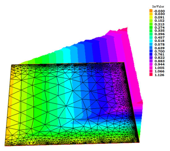
Figure 21. A 3D plot of the computed solution for example 4.

The results of the refined meshes are shown in Figure 22 and Figure 23 for the residual-based, gradient-based and ${\eta }_N$ error estimators, respectively.

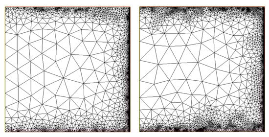
Figure 22. Example 4: results with the residual-based error estimator. (Left) The final mesh obtained by using c = auto is shown. (Right) The final mesh with c = 0.3.

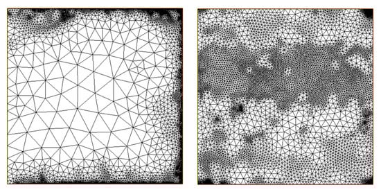
Figure 23. Example 4. (Left) The final mesh obtained with the gradient-based error estimator. (Right) The final mesh obtained with the Neumann auxiliary error estimator.

In Table 10, we report the results obtained by using $c=$ auto and $c=0.3$ when ${\eta }_R$ is employed. By setting a contamination value that differs from the default setting, we can better refine the regions with the interested layers.

Table 10. Error in $L^2$ norm and $H^1$ seminorm for example 4 obtained with the residual-based error estimator.

c = auto				c = 0.3
$n$	NT	$L^2$	$H^1$	NT	$L^2$	$H^1$
0	200	5.2 × 10${}^{-2}$	6.4 × 10${}^{-1}$	-	-	-
1	375	5.3 × 10${}^{-2}$	3.4 × 10${}^{-1}$	232	4.7 × 10${}^{-2}$	1.9 × 10${}^{-1}$
2	1125	2.9 × 10${}^{-2}$	1.9 × 10${}^{-2}$	970	5.2 × 10${}^{-2}$	1.4 × 10${}^{-1}$
3	2912	3.3 × 10${}^{-2}$	1.9 × 10${}^{-2}$	1436	2.7 × 10${}^{-2}$	1.2 × 10${}^{-2}$
4	8798	3.9 × 10${}^{-2}$	1.5 × 10${}^{-2}$	5246	3.7 × 10${}^{-2}$	1.0 × 10${}^{-2}$
5	15,276	4.1 × 10${}^{-2}$	2.6 × 10${}^{-3}$	16,689	3.9 × 10${}^{-2}$	3.9 × 10${}^{-4}$

Finally, in Table 11 and Table 12, we report the error estimates computed with ${\eta }_Z$ and ${\eta }_N$, respectively, and c = auto. This final benchmark is the only one where the use of ${\eta }_N$ failed to capture the boundary layers. In fact, the values of ${\eta }_{N,T}$ are very small almost for every triangle T, at every level; thus, at the end, the adaptive refinement almost appeared as a uniform global refinement. In this case, even the use of a contamination parameter could not help to significantly improve the final result. The test was also repeated with smaller values of contamination, but the final mesh was still not satisfactory. In Figure 23, on the right, the final mesh obtained at level $n=5$ with $c=0.1$ is shown. We cannot appreciate a significant difference with the error obtained with ${\eta }_R$ or ${\eta }_Z$ but simply because we are comparing with a solution obtained exactly by uniformly and globally refining the initial mesh. Only the mesh obtained with ${\eta }_R$ and ${\eta }_Z$ is correctly refined at the boundary layer location.

Table 11. Error in $L^2$ norm and $H^1$ seminorm for example 4 obtained with ${\eta }_Z$.

n	NT	${\mathit{L}}^2$	${\mathit{H}}^1$
0	200	5.2 × 10${}^{-2}$	6.4 × 10${}^{-1}$
1	557	3.5 × 10${}^{-2}$	1.9 × 10${}^{-1}$
2	2304	3.4 × 10${}^{-2}$	3.1 × 10${}^{-2}$
3	8813	2.2 × 10${}^{-2}$	2.3 × 10${}^{-3}$
4	15,731	2.6 × 10${}^{-2}$	1.9 × 10${}^{-3}$

Table 12. Error in $L^2$ norm and $H^1$ seminorm for example 4 obtained with ${\eta }_N$.

n	NT	${\mathit{L}}^2$	${\mathit{H}}^1$
0	200	5.2 × 10${}^{-2}$	6.4 × 10${}^{-1}$
1	264	6.1 × 10${}^{-2}$	3.1 × 10${}^{-1}$
2	459	6.6 × 10${}^{-2}$	2.3 × 10${}^{-1}$
3	803	5.1 × 10${}^{-2}$	3.3 × 10${}^{-2}$
4	1298	5.0 × 10${}^{-2}$	4.3 × 10${}^{-2}$
5	4428	4.4 × 10${}^{-2}$	4.5 × 10${}^{-2}$
6	11,323	3.6 × 10${}^{-2}$	1.8 × 10${}^{-2}$

In Figure 24, we show the comparison of ${\eta }_R$ against the global refinement strategy. In this example, the $L^2$ norm of the global refinement is more accurate than the adaptive mesh obtained either with c = auto or with c = 0.3. The $H^1$ seminorm of the global refinement is very unstable, instead.

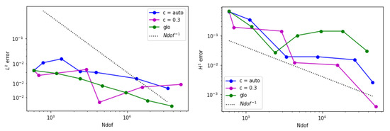
Figure 24. Error behavior for example 4 when ${\eta }_R$ is adopted. (Left) The estimated $L^2$ norm of the error is displayed. (Right) The estimated $H^1$ seminorm is shown.

In Figure 25, the mesh adapted with ${\eta }_Z$ is able to produce a smaller error in the $H^1$ seminorm than the global refinement, while the final reached accuracy is comparable in the case of the $L^2$ norm.

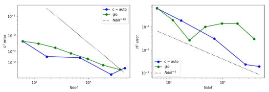
Figure 25. Error behavior for example 4 when ${\eta }_Z$ is adopted. (Left) The estimated $L^2$ norm of the error is displayed. (Right) The estimated $H^1$ seminorm is shown.

In Figure 26, we can observe how the behavior of ${\eta }_N$ is very similar to the global refinement strategy, at least for this last example. Therefore, in this case, both strategies give comparable results in terms of accuracy and in terms of the order of convergence.

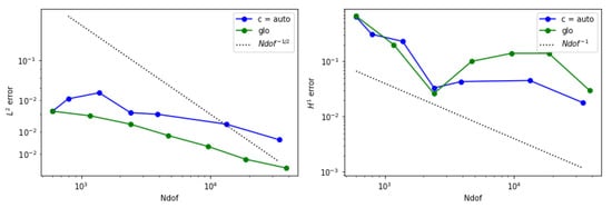
Figure 26. Error behavior for example 4 when ${\eta }_N$ is adopted. (Left) The estimated $L^2$ norm of the error is displayed. (Right) The estimated $H^1$ seminorm is shown.

4. Discussion

The numerical results obtained with the proposed strategy are interesting and rather promising. The introduction of an anomaly detection technique, with default parameters, in place of deciding for a marking strategy, improves the robustness of the performance of the three error estimators in terms of the reached accuracy per level of refinement. Further research should be devoted to designing suitable algorithms to choose different contamination settings, either for the IF or for other unsupervised techniques. At the current stage, we do not exploit the contamination parameter c at its best as only the top percentage c anomalies are the triangles that will be refined. To improve the robustness of the choice of which triangle should be neglected, an extra module should be added to the algorithm in order to interact with the connectivity matrix for the produced triangulation inside the FEM procedure. Moreover, other tools of unsupervised learning approaches could be added; see, e.g., the recent work [33]. Thus far, by only using a fully automatic setting, the residual-based error estimator ${\eta }_R$ was the only one to correctly detect all the boundary layers analyzed. A deeper statistical analysis could also be conducted by taking into account more examples belonging to the same category, e.g., reaction-dominant problems or convective-dominant problems, or only problems with circular layers or parabolic layers, etc. Hence, the creation of a rich database would allow us to test and to objectively validate the obtained results. Having robust strategies that allow for better control and thus a smaller number of degrees of freedom is of fundamental importance, not only from the computational point of view but also for better accuracy in reproducing the observed physical phenomenon.

References

- Brooks, A.N.; Hughes, T.J.R. Streamline upwind/Petrov-Galerkin formulations for convection dominated flows with particular emphasis on the incompressible Navier-Stokes equations. Comput. Methods Appl. Mech. Eng. 1982, 32, 199–259. [Google Scholar] [CrossRef]
- Araya, R.; Aguayo, J.; Muñoz, S. An adaptive stabilized method for advection–diffusion–reaction equation. J. Comput. Appl. Math. 2020, 376, 112858. [Google Scholar] [CrossRef]
- Speleers, H.; Manni, C.; Pelosi, F.; Sampoli, M.L. Isogeometric analysis with Powell–Sabin splines for advection–diffusion–reaction problems. Comput. Methods Appl. Mech. Eng. 2012, 221, 132–148. [Google Scholar] [CrossRef]
- Manni, C.; Pelosi, F.; Sampoli, M.L. Isogeometric analysis in advection–diffusion problems: Tension splines approximation. J. Comput. Appl. Math. 2011, 236, 511–528. [Google Scholar] [CrossRef] [Green Version]
- Zhang, Q.; Johansen, H.; Colella, P. A fourth-order accurate finite-volume method with structured adaptive mesh refinement for solving the advection-diffusion equation. SIAM J. Sci. Comput. 2012, 34, B179–B201. [Google Scholar] [CrossRef] [Green Version]
- John, V. A numerical study of a posteriori error estimators for convection-diffusion equations. Comput. Methods Appl. Mech. Eng. 2000, 190, 757–781. [Google Scholar] [CrossRef]
- John, V.; Novo, J. A robust SUPG norm a posteriori error estimator for stationary convection-diffusion equations. Comput. Methods Appl. Mech. Eng. 2013, 255, 289–305. [Google Scholar] [CrossRef]
- Araya, R.; Poza, A.H.; Stephan, E.P. A hierarchical a posteriori error estimate for an advection-diffusion-reaction problem. Math. Models Methods Appl. Sci. 2005, 15, 1119–1139. [Google Scholar] [CrossRef]
- Gonzalez, M.; Strugaru, M. Stabilization and a posteriori error analysis of a mixed FEM for convection–Diffusion problems with mixed boundary conditions. J. Comput. Appl. Math. 2021, 381, 113015. [Google Scholar] [CrossRef]
- Jha, A. A residual based a posteriori error estimators for AFC schemes for convection-diffusion equations. Comput. Math. Appl. 2021, 97, 86–99. [Google Scholar] [CrossRef]
- Tobiska, L.; Verfürth, R. Robust a posteriori error estimates for stabilized finite element methods. IMA J. Numer. Anal. 2015, 35, 1652–1671. [Google Scholar] [CrossRef] [Green Version]
- Verfürth, R. A posteriori error estimators for convection-diffusion equations. Numer. Math. 1998, 80, 641–663. [Google Scholar] [CrossRef]
- Morin, P.; Nochetto, R.H.; Siebert, K.G. Data oscillation and convergence of adaptive FEM. SIAM J. Numer. Anal. 2000, 38, 466–488. [Google Scholar] [CrossRef]
- Chandola, V.; Banerjee, A.; Kumar, V. Anomaly detection: A survey. ACM Comput. Surv. (CSUR) 2009, 41, 1–58. [Google Scholar] [CrossRef]
- Anitescu, C.; Atroshchenko, E.; Alajlan, N.; Rabczuk, T. Artificial neural network methods for the solution of second order boundary value problems. Comput. Mater. Contin. 2019, 59, 345–359. [Google Scholar] [CrossRef] [Green Version]
- Paszyński, M.; Grzeszczuk, R.; Pardo, D.; Demkowicz, L. Deep learning driven self-adaptive hp finite element method. In International Conference on Computational Science; Springer: Cham, Switzerland, 2021; pp. 114–121. [Google Scholar]
- Zhang, Z.; Wang, Y.; Jimack, P.K.; Wang, H. MeshingNet: A new mesh generation method based on deep learning. In International Conference on Computational Science; Springer: Cham, Switzerland, 2020; pp. 186–198. [Google Scholar]
- Papastavrou, A.; Verfürth, R. A posteriori error estimators for stationary convection-diffusion problems: A computational comparison. Comput. Methods Appl. Mech. Eng. 2000, 189, 449–462. [Google Scholar] [CrossRef]
- Verfürth, R. A Posteriori Error Estimation and Adaptive Mesh-refinement Techniques. J. Comput. Appl. Math. 1994, 50, 67–83. [Google Scholar] [CrossRef]
- Hecht, F. New development in Freefem++. J. Numer. Math. 2012, 20, 251–265. [Google Scholar] [CrossRef]
- George, P.L. Automatic mesh generation and finite element computation. Handb. Numer. Anal. 1996, 4, 69–190. [Google Scholar]
- Hecht, F. BAMG: Bidimensional Anisotropic Mesh Generator. User Guide. INRIA Report. 1998. Available online: https://www.google.com.hk/url?sa=t&rct=j&q=&esrc=s&source=web&cd=&ved=2ahUKEwiPwYzcoYX0AhWFZd4KHQXmChEQFnoECAYQAQ&url=http%3A%2F%2Fftp.tw.freebsd.org%2Fdistfiles%2Fbamg.pdf&usg=AOvVaw3ImBK9-1HO6KN5FtzyC7iu (accessed on 4 November 2021).
- Liu, F.T.; Ting, K.M.; Zhou, Z.H. Isolation forest. In Proceedings of the 2008 Eighth IEEE International Conference on Data Mining, Pisa, Italy, 15–19 December 2008; pp. 413–422. [Google Scholar]
- Liu, F.T.; Ting, K.M.; Zhou, Z.H. Isolation-based anomaly detection. ACM Trans. Knowl. Discov. Data (TKDD) 2012, 6, 1–39. [Google Scholar] [CrossRef]
- Pedregosa, F.; Varoquaux, G.; Gramfort, A.; Michel, V.; Thirion, B.; Grisel, O.; Blondel, M.; Prettenhofer, P.; Weiss, R.; Dubourg, V.; et al. Scikit-learn: Machine Learning in Python. J. Mach. Learn. Res. 2011, 12, 2825–2830. [Google Scholar]
- Taylor, M.A.; Wingate, B.A.; Bos, L.P. Several New Quadrature Formulas for Polynomial Integration in the Triangle. Report No: SAND2005-0034J. Available online: http://xyz.lanl.gov/format/math.NA/0501496 (accessed on 8 February 2007).
- Falini, F.; Kanduč, T. A study on spline quasi-interpolation based quadrature rules for the isogeometric Galerkin BEM. In Advanced Methods for Geometric Modeling and Numerical Simulation; Springer: Cham, Switzerland, 2019; pp. 99–125. [Google Scholar]
- Hussain, F.; Karim, M.S.; Ahamad, R. Appropriate Gaussian quadrature formulae for triangles. Int. J. Appl. Math. Comput. 2012, 4, 24–38. [Google Scholar]
- Huybrechs, D. Stable high-order quadrature rules with equidistant points. J. Comput. Appl. Math. 2009, 231, 933–947. [Google Scholar] [CrossRef] [Green Version]
- McCorquodale, P.; Colella, P. A high-order finite-volume method for conservation laws on locally refined grids. Commun. Appl. Math. Com. Sci. J. 2011, 6, 1–25. [Google Scholar] [CrossRef] [Green Version]
- Bazilevs, Y.; Calo, V.M.; Cottrell, J.A.; Evans, J.A.; Hughes, T.J.R.; Lipton, S.; Scott, M.A.; Sederberg, T.W. Isogeometric analysis using T-splines. Comput. Methods Appl. Mech. Eng. 2010, 199, 229–263. [Google Scholar] [CrossRef] [Green Version]
- Formaggia, L.; Micheletti, S.; Perotto, S. Anisotropic mesh adaptation in computational fluid dynamics: Application to the advection-diffusion-reaction and the Stokes problem. Appl. Numer. Math. 2004, 51, 511–533. [Google Scholar] [CrossRef]
- Falini, A.; Mazzia, F.; Tamborrino, C. Spline based Hermite quasi-interpolation for univariate time series. Discret. Contin. Dyn. Syst. submitted.
Publisher’s Note: MDPI stays neutral with regard to jurisdictional claims in published maps and institutional affiliations. |
© 2021 by the authors. Licensee MDPI, Basel, Switzerland. This article is an open access article distributed under the terms and conditions of the Creative Commons Attribution (CC BY) license (https://creativecommons.org/licenses/by/4.0/).