
Simultaneous Feature Selection and Support Vector Machine Optimization Using an Enhanced Chimp Optimization Algorithm


Abstract
:1. Introduction
- An Enhanced Chimp Optimization Algorithm is proposed to solve the shortcomings of the ChOA and make it better applied to feature selection problems.
- HDPM strategy is introduced in the initial stage to enhance the population diversity.
- Spearman’s rank correlation coefficient helps to identify the chimps that need to be improved. Then BAS is introduced to improve the positions updating ability.
- The EChOA-SVM model is used for feature selection and SVM parameter optimization simultaneously. The model is evaluated by 17 benchmark data sets in UCI machine learning library [34]. In order to verify the effectiveness of this method, it is compared with seven optimization algorithms, such as ChOA [31], GWO [35], WOA [36], ALO [37], GOA [38], MFO [39], and SSA [40].
2. Literature Review
3. Chimp Optimization Algorithm (ChOA)
4. Enhanced Chimp Optimization Algorithm (EChOA)
4.1. Highly Disruptive Polynomial Mutation (HDPM)
4.2. Spearman’s Rank Correlation Coefficient
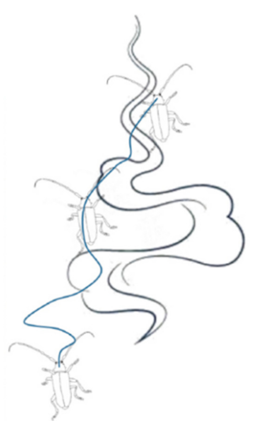
4.3. Beetle Antennae Search Algorithm (BAS)
4.4. Improvement Strategy
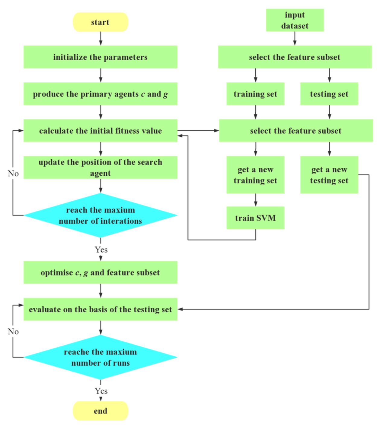
4.5. EChOA for Optimizing SVM and Feature Selection
- Initialize the population, position and fitness value of the chimps.
- SVM randomly generates the values of c and g, and then calculates the initial fitness value.
- The training model is obtained by training set in support vector machine.
- Reorder the population to get the agent position and fitness value after sorting.
5. Experimental Results and Discussion
5.1. Datasets Details
5.2. Parameters Setting
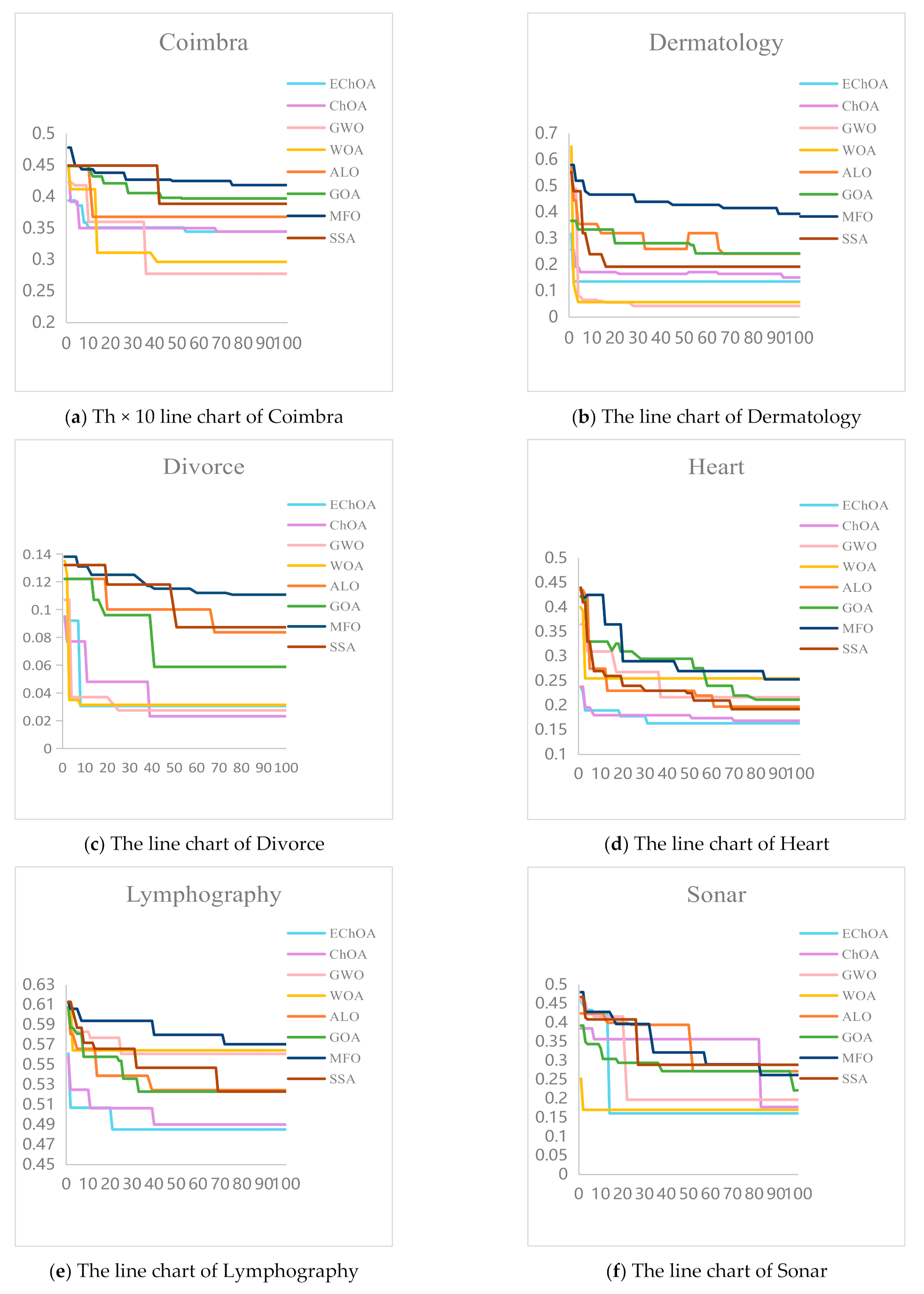
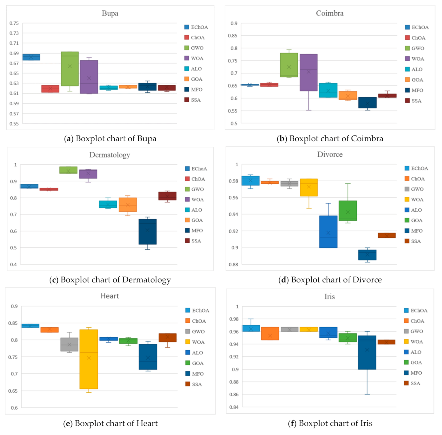
5.3. Results and Discussion
- Accuracy: Accuracy represents the ratio between the number of correct classification and the actual number, which is reflecting the accuracy of the classifier recognition results. It is an important index to evaluate algorithm performance;
- The number of features: The number of features reflects ability of eliminate redundancy. It shows whether the method can find the optimal feature subset;
- Fitness value: Fitness value can reflect the advantages and disadvantages of the solution selected by the classifier. The better fitness value can get the better the solution.
6. Conclusions
Author Contributions
Funding
Institutional Review Board Statement
Informed Consent Statement
Data Availability Statement
Conflicts of Interest
References
- Raju, B.; Bonagiri, R. A cavernous analytics using advanced machine learning for real world datasets in research implementations. Mater. Today Proc. 2020. [Google Scholar] [CrossRef]
- Jiang, J.; Yu, C.; Xu, X.; Ma, Y.; Liu, J. Achieving better connections between deposited lines in additive manufacturing via machine learning. Math. Biosci. Eng. 2020, 17, 3382–3394. [Google Scholar] [CrossRef] [PubMed]
- Kline, A.S.; Kline, T.J.B.; Lee, J. Item response theory as a feature selection and interpretation tool in the context of machine learning. Med. Biol. Eng. Comput. 2021, 59, 471–482. [Google Scholar] [CrossRef]
- Ebrahimi-Khusfi, Z.; Nafarzadegan, A.R.; Dargahian, F. Predicting the number of dusty days around the desert wetlands in southeastern Iran using feature selection and machine learning techniques. Ecol. Indic. 2021, 125, 1–15. [Google Scholar] [CrossRef]
- Tanveer, M. Robust and Sparse Linear Programming Twin Support Vector Machines. Cogn. Comput. 2015, 7, 137–149. [Google Scholar] [CrossRef]
- Yang, P.; Li, Z.; Yu, Y.; Shi, J.; Sun, M. Studies on fault diagnosis of dissolved oxygen sensor based on GA-SVM. Math. Biosci. Eng. 2021, 18, 386–399. [Google Scholar] [CrossRef] [PubMed]
- Aziz, W.; Hussain, L.; Khan, I.R.; Alowibdi, J.S.; Alkinani, M.H. Machine learning based classification of normal, slow and fast walking by extracting multimodal features from stride interval time series. Math. Biosci. Eng. 2021, 18, 495–517. [Google Scholar] [CrossRef]
- Hussain, L.; Aziz, W.; Khan, I.R.; Alkinani, M.H.; Alowibdi, J.S. Machine learning based congestive heart failure detection using feature importance ranking of multimodal features. Math. Biosci. Eng. 2021, 18, 69–91. [Google Scholar] [CrossRef] [PubMed]
- Brown, M.P.S.; Grundy, W.N.; Lin, D.; Cristianini, N.; Sugnet, C.W.; Furey, T.; Ares, M.; Haussler, D. Knowledge-based analysis of microarray gene expression data by using support vector machines. Proc. Natl. Acad. Sci. USA. 2000, 97, 262–267. [Google Scholar] [CrossRef] [Green Version]
- Takeuchi, K.; Collier, N. Bio-medical entity extraction using support vector machines. Artif. Intell. Med. 2005, 33, 125–137. [Google Scholar] [CrossRef] [PubMed]
- Babaoğlu, I.; Findik, O.; Bayrak, M. Effects of principle component analysis on assessment of coronary artery diseases using support vector machine. Expert Syst. Appl. 2010, 37, 2182–2185. [Google Scholar] [CrossRef]
- Du, Z.; Yang, Q.; He, H.; Qiu, M.; Chen, Z.; Hu, Q.; Wang, Q.; Zhang, Z.; Lin, Q.; Huang, L.; et al. A comprehensive health classification model based on support vector machine for proseal laryngeal mask and tracheal catheter assessment in herniorrhaphy. Math. Biosci. Eng. 2020, 17, 1838–1854. [Google Scholar] [CrossRef]
- Sotiris, V.A.; Tse, P.W.; Pecht, M. Anomaly Detection through a Bayesian Support Vector Machine. IEEE Trans. Reliab. 2010, 59, 277–286. [Google Scholar] [CrossRef]
- Rostami, O.; Kaveh, M. Optimal feature selection for SAR image classification using biogeography-based optimization (BBO), artificial bee colony (ABC) and support vector machine (SVM): A combined approach of optimization and machine learning. Comput. Geosci. 2021, 25, 911–930. [Google Scholar] [CrossRef]
- Joachims, T. Making Large-Scale Support Vector Machine Learning Practical; MIT Press: Cambridge, MA, USA, 1999; pp. 169–184. [Google Scholar]
- Weston, J.; Mukherjee, S.; Chapelle, O. Feature selection for SVMs. Adv. Neural Inf. Process Syst. 2000, 13, 668–674. [Google Scholar]
- Nguyen, M.H.; Torre, F.D.L. Optimal feature selection for support vector machines. Pattern Recognit. 2010, 43, 584–591. [Google Scholar] [CrossRef]
- Shahbeig, S.; Helfroush, M.S.; Rahideh, A. A fuzzy multi-objective hybrid TLBO–PSO approach to select the associated genes with breast cancer. Signal Process. 2017, 131, 58–65. [Google Scholar] [CrossRef]
- Wu, Q.; Ma, Z.; Fan, J.; Xu, G.; Shen, Y. A feature selection method based on hybrid improved binary quantum particle swarm optimization. IEEE Access 2019, 7, 80588–80601. [Google Scholar] [CrossRef]
- Souza, T.A.; Souza, M.A.; Costa, W.C.D.A.; Costa, S.C.; Correia, S.E.N.; Vieira, V.J.D. Feature Selection based on Binary Particle Swarm Optimization and Neural Networks for Pathological Voice Detection. Int. J. Bio-Inspired Comput. 2018, 11, 2. [Google Scholar] [CrossRef]
- Wang, H.; Niu, B.; Tan, L. Bacterial colony algorithm with adaptive attribute learning strategy for feature selection in classification of customers for personalized recommendation. Neurocomputing 2021, 452, 747–755. [Google Scholar] [CrossRef]
- Jha, K.; Saha, S. Incorporation of multimodal objective optimization in designing a filter based feature selection technique. Appl. Soft Comput. 2021, 98, 106823. [Google Scholar] [CrossRef]
- Han, M.; Liu, X. Feature selection techniques with class separability for multivariate time series. Neurocomputing 2013, 110, 29–34. [Google Scholar] [CrossRef]
- Nithya, B.; Ilango, V. Evaluation of machine learning based optimized feature selection approaches and classification methods for cervical cancer prediction. SN Appl. Sci. 2019, 1, 641. [Google Scholar] [CrossRef] [Green Version]
- Kohavi, R.; John, G.H. Wrappers for feature subset selection. Artif. Intell. 1997, 97, 273–324. [Google Scholar] [CrossRef] [Green Version]
- Pourpanah, F.; Lim, C.P.; Wang, X.; Tan, C.J.; Seera, M.; Shi, Y. A hybrid model of fuzzy min–max and brain storm optimization for feature selection and data classification. Neurocomputing 2019, 333, 440–451. [Google Scholar] [CrossRef]
- Liu, H.; Setiono, R. A probabilistic approach to feature selection-a filter solution. In Proceedings of the 9th International Conference on Industrial and Engineering Applications of AI and ES, Fukuoka, Japan, 4–7 June 1996. [Google Scholar]
- Wang, J.; Wu, L.; Kong, J.; Li, Y.; Zhang, B. Maximum weight and minimum redundancy: A novel framework for feature subset selection. Pattern Recognit. 2013, 46, 1616–1627. [Google Scholar] [CrossRef]
- Sihwail, R.; Omar, K.; Ariffin, K.A.Z.; Tubishat, M. Improved Harris Hawks Optimization Using Elite Opposition-Based Learning and Novel Search Mechanism for Feature Selection. IEEE Access 2020, 8, 121127–121145. [Google Scholar] [CrossRef]
- Elgamal, Z.M.; Yasin, N.B.M.; Tubishat, M.; Alswaitti, M.; Mirjalili, S. An Improved Harris Hawks Optimization Algorithm with Simulated Annealing for Feature Selection in the Medical Field. IEEE Access 2020, 8, 186638–186652. [Google Scholar] [CrossRef]
- Khishe, M.; Mosavi, M. Chimp optimization algorithm. Expert Syst. Appl. 2020, 149, 113338. [Google Scholar] [CrossRef]
- Abed-Alguni, B. Island-based Cuckoo Search with Highly Disruptive Polynomial Mutation. Int. J. Artif. Intell. 2019, 17, 57–82. [Google Scholar]
- Jiang, X.; Li, S. BAS: Beetle Antennae Search Algorithm for Optimization Problems. arXiv 2017, arXiv:1710.10724. [Google Scholar] [CrossRef]
- Lichman, M. UCI Machine Learning Repository. Available online: http://archive.ics.uci.edu/ml (accessed on 15 August 2013).
- Renita, D.B.; Christopher, C.S. Novel real time content based medical image retrieval scheme with GWO-SVM. Multimed. Tools Appl. 2020, 79, 17227–17243. [Google Scholar] [CrossRef]
- Yin, X.; Hou, Y.; Yin, J.; Li, C. A novel SVM parameter tuning method based on advanced whale optimization algorithm. J. Phys. Conf. Ser. 2019, 1237, 022140. [Google Scholar] [CrossRef] [Green Version]
- Zhao, S.; Gao, L.; Dongmei, Y.; Jun, T. Ant Lion Optimizer with Chaotic Investigation Mechanism for Optimizing SVM Parameters. J. Front. Comput. Sci. Technol. 2016, 10, 722–731. [Google Scholar]
- Aljarah, I.; Al-Zoubi, A.M.; Faris, H.; Hassonah, M.A.; Mirjalili, S.; Saadeh, H. Simultaneous Feature Selection and Support Vector Machine Optimization Using the Grasshopper Optimization Algorithm. Cogn. Comput. 2018, 10, 478–495. [Google Scholar] [CrossRef] [Green Version]
- Lin, G.Q.; Li, L.L.; Tseng, M.L.; Liu, H.M.; Yuan, D.D.; Tan, R.R. An improved moth-flame optimization algorithm for support vector machine prediction of photovoltaic power generation. J. Clean. Prod. 2020, 253, 119966. [Google Scholar] [CrossRef]
- Sivapragasam, C.; Liong, S.-Y.; Pasha, M.F.K. Rainfall and runoff forecasting with SSA–SVM approach. J. Hydroinformatics 2001, 3, 141–152. [Google Scholar] [CrossRef] [Green Version]
- Zhao, H.; Zhang, C. An online-learning-based evolutionary many-objective algorithm. Inf. Sci. 2020, 509, 1–21. [Google Scholar] [CrossRef]
- Dulebenets, M.A. An Adaptive Polyploid Memetic Algorithm for scheduling trucks at a cross-docking terminal. Inf. Sci. 2021, 565, 390–421. [Google Scholar] [CrossRef]
- Liu, Z.-Z.; Wang, Y.; Huang, P.-Q. AnD: A many-objective evolutionary algorithm with angle-based selection and shift-based density estimation. Inf. Sci. 2020, 509, 400–419. [Google Scholar] [CrossRef] [Green Version]
- Pasha, J.; Dulebenets, M.A.; Kavoosi, M.; Abioye, O.F.; Wang, H.; Guo, W. An Optimization Model and Solution Algorithms for the Vehicle Routing Problem with a “Factory-in-a-Box”. IEEE Access 2020, 8, 134743–134763. [Google Scholar] [CrossRef]
- D’Angelo, G.; Pilla, R.; Tascini, C.; Rampone, S. A proposal for distinguishing between bacterial and viral meningitis using genetic programming and decision trees. Soft Comput. 2019, 23, 11775–11791. [Google Scholar] [CrossRef]
- Panda, N.; Majhi, S.K. How effective is the salp swarm algorithm in data classification. In Computational Intelligence in Pattern Recognition; Springer: Singapore, 2020; pp. 579–588. [Google Scholar]
- Alwan, H.B.; Mahamud, K. Mixed-variable ant colony optimisation algorithm for feature subset selection and tuning support vector machine parameter. Int. J. Bio-Inspired Comput. 2017, 9, 53–63. [Google Scholar] [CrossRef]
- Frhlich, H.; Chapelle, O.; Schlkopf, B. Feature Selection for Support Vector Machines by Means of Genetic Algorithms. In Proceedings of the 15th IEEE International Conference on Tools with Artificial Intelligence (ICTAI 2003), Sacramento, CA, USA, 5 November 2003; IEEE: New York, NY, USA, 2003. [Google Scholar]
- Huang, C.-L.; Wang, C.-J. A GA-based feature selection and parameters optimizationfor support vector machines. Expert Syst. Appl. 2006, 31, 231–240. [Google Scholar] [CrossRef]
- Lin, S.-W.; Tseng, T.-Y.; Chen, S.-C.; Huang, J.-F. A SA-Based Feature Selection and Parameter Optimization Approach for Support Vector Machine. Pervasive Comput. IEEE 2006. [Google Scholar] [CrossRef]
- Jia, H.; Sun, K. Improved barnacles mating optimizer algorithm for feature selection and support vector machine optimization. Pattern Anal. Appl. 2021, 24, 1249–1274. [Google Scholar] [CrossRef] [PubMed]
- Slipinski, A.; Escalona, H. Australian Longhorn Beetles (Coleoptera: Cerambycidae); CSIRO Publishing: Clayton, Australia, 2013; Volume 1. [Google Scholar]
- Mafarja, M.M.; Mirjalili, S. Hybrid Whale Optimization Algorithm with simulated annealing for feature selection. Neurocomputing 2017, 260, 302–312. [Google Scholar] [CrossRef]


| Data Set | Features | Instances | Classes |
|---|---|---|---|
| Balance | 4 | 625 | 3 |
| Bupa | 6 | 345 | 2 |
| Coimbra | 9 | 116 | 2 |
| Dermatology | 34 | 358 | 6 |
| Diagnostic | 10 | 683 | 4 |
| Divorce | 18 | 170 | 2 |
| Glass | 10 | 214 | 6 |
| Heart | 13 | 270 | 2 |
| Iris | 4 | 150 | 3 |
| Knowledge | 5 | 258 | 4 |
| Liver | 6 | 345 | 2 |
| Lymphography | 18 | 148 | 8 |
| Sonar | 60 | 208 | 2 |
| Teaching Assistant Evaluation (TAE) | 5 | 151 | 3 |
| Transfusion | 4 | 748 | 2 |
| Wine | 13 | 178 | 3 |
| Zoo | 16 | 101 | 7 |
| Algorithm | Parameters | Value |
|---|---|---|
| EChOA | ηm | 1 |
| C | 2 | |
| K | 0.95 | |
| f | [0, 2.5] | |
| m | Gauss chaotic | |
| ChOA | f | [0, 2.5] |
| m | Gauss chaotic | |
| GWO | α | [0, 2] |
| WOA | α | [0, 2] |
| a2 | [−2, −1] | |
| ALO | Number of search agents | 30 |
| Number of iterations | 100 | |
| GOA | cMin | 0.00001 |
| cMax | 1 | |
| Number of search agents | 30 | |
| Number of iterations | 100 | |
| MFO | α | [−2, −1] |
| b | 1 | |
| t | [−2, −1] | |
| SSA | c1 | [2 × 10⁻¹⁶, 2] |
| c2 | [0, 1] | |
| c3 | [0, 1] |
| EChOA | ChOA | GWO | WOA | ALO | GOA | MFO | SSA | ||
|---|---|---|---|---|---|---|---|---|---|
| Balance | mean | 8.9853 × 10⁻¹ | 8.9073 × 10⁻¹ | 8.8640 × 10⁻¹ | 8.9376 × 10⁻¹ | 8.9120 × 10⁻¹ | 8.9120 × 10⁻¹ | 7.7344 × 10⁻¹ | 8.9120 × 10⁻¹ |
| std | 6.4825 × 10⁻³ | 4.1199 × 10⁻³ | 1.5513 × 10⁻² | 2.6349 × 10⁻³ | 1.2413 × 10⁻¹⁶ | 1.2413 × 10⁻¹⁶ | 6.5830 × 10⁻² | 1.2413 × 10⁻¹⁶ | |
| Bupa | mean | 6.8217 × 10⁻¹ | 6.1943 × 10⁻¹ | 6.6380 × 10⁻¹ | 6.4002 × 10⁻¹ | 6.2106 × 10⁻¹ | 6.2260 × 10⁻¹ | 6.2378 × 10⁻¹ | 6.2204 × 10⁻¹ |
| std | 5.8192 × 10⁻³ | 7.1396 × 10⁻³ | 3.6625 × 10⁻² | 3.3470 × 10⁻² | 3.9715 × 10⁻³ | 3.2047 × 10⁻³ | 8.5538 × 10⁻³ | 5.7270 × 10⁻³ | |
| Coimbra | mean | 6.5348 × 10⁻¹ | 6.5348 × 10⁻¹ | 7.2414 × 10⁻¹ | 7.0518 × 10⁻¹ | 6.2930 × 10⁻¹ | 6.0818 × 10⁻¹ | 5.7930 × 10⁻¹ | 6.0858 × 10⁻¹ |
| std | 3.8460 × 10⁻³ | 7.1953 × 10⁻³ | 5.2065 × 10⁻² | 9.1744 × 10⁻² | 2.8621 × 10⁻² | 1.7562 × 10⁻² | 2.3106 × 10⁻² | 1.1583 × 10⁻² | |
| Dermatology | mean | 8.6590 × 10⁻¹ | 8.5010 × 10⁻¹ | 9.6087 × 10⁻¹ | 9.4638 × 10⁻¹ | 7.5922 × 10⁻¹ | 7.5752 × 10⁻¹ | 6.0560 × 10⁻¹ | 8.0838 × 10⁻¹ |
| std | 1.2205 × 10⁻² | 6.9936 × 10⁻³ | 2.1811 × 10⁻² | 3.1929 × 10⁻² | 2.4481 × 10⁻² | 4.6042 × 10⁻² | 8.1800 × 10⁻² | 2.6113 × 10⁻² | |
| Diagnostic | mean | 9.6607 × 10⁻¹ | 9.5450 × 10⁻¹ | 9.6516 × 10⁻¹ | 9.6430 × 10⁻¹ | 9.5842 × 10⁻¹ | 9.5754 × 10⁻¹ | 9.3558 × 10⁻¹ | 9.5842 × 10⁻¹ |
| std | 6.1598 × 10⁻³ | 4.4034 × 10⁻³ | 3.7997 × 10⁻³ | 6.0828 × 10⁻³ | 1.2969 × 10⁻³ | 2.0683 × 10⁻³ | 9.6469 × 10⁻³ | 1.2969 × 10⁻³ | |
| Divorce | mean | 9.8044 × 10⁻¹ | 9.7768 × 10⁻¹ | 9.7650 × 10⁻¹ | 9.7298 × 10⁻¹ | 9.1764 × 10⁻¹ | 9.4236 × 10⁻¹ | 8.9176 × 10⁻¹ | 9.1412 × 10⁻¹ |
| std | 6.3689 × 10⁻³ | 2.6386 × 10⁻³ | 4.1719 × 10⁻³ | 1.4765 × 10⁻² | 2.1989 × 10⁻² | 1.9255 × 10⁻² | 6.6920 × 10⁻³ | 3.1768 × 10⁻³ | |
| Glass | mean | 6.8067 × 10⁻¹ | 6.7290 × 10⁻¹ | 9.8813 × 10⁻¹ | 7.5796 × 10⁻¹ | 6.3924 × 10⁻¹ | 6.5048 × 10⁻¹ | 5.8410 × 10⁻¹ | 6.7010 × 10⁻¹ |
| std | 1.1775 × 10⁻² | 1.2341 × 10⁻² | 2.3159 × 10⁻³ | 7.1049 × 10⁻¹ | 1.5296 × 10⁻² | 2.5891 × 10⁻² | 4.9679 × 10⁻² | 3.7157 × 10⁻² | |
| Heart | mean | 8.4230 × 10⁻¹ | 8.3207 × 10⁻¹ | 7.8594 × 10⁻¹ | 7.4666 × 10⁻¹ | 8.0370 × 10⁻¹ | 7.9738 × 10⁻¹ | 7.4740 × 10⁻¹ | 8.0888 × 10⁻¹ |
| std | 4.7606 × 10⁻³ | 8.5448 × 10⁻³ | 2.2868 × 10⁻² | 8.8013 × 10⁻² | 6.4086 × 10⁻³ | 9.3041 × 10⁻³ | 3.8271 × 10⁻² | 1.7667 × 10⁻² | |
| Iris | mean | 9.6400 × 10⁻¹ | 9.5337 × 10⁻¹ | 9.6268 × 10⁻¹ | 9.6268 × 10⁻¹ | 9.5734 × 10⁻¹ | 9.4934 × 10⁻¹ | 9.3068 × 10⁻¹ | 9.4268 × 10⁻¹ |
| std | 8.9443 × 10⁻³ | 1.1547 × 10⁻² | 3.6697 × 10⁻³ | 3.6697 × 10⁻³ | 8.9592 × 10⁻³ | 7.5910 × 10⁻³ | 4.0173 × 10⁻² | 3.6697 × 10⁻³ | |
| Knowledge | mean | 9.5675 × 10⁻¹ | 9.5087 × 10⁻¹ | 8.5426 × 10⁻¹ | 8.9692 × 10⁻¹ | 9.5350 × 10⁻¹ | 9.4660 × 10⁻¹ | 9.0542 × 10⁻¹ | 9.5428 × 10⁻¹ |
| std | 1.8385 × 10⁻³ | 2.3714 × 10⁻³ | 7.9861 × 10⁻² | 4.6400 × 10⁻² | 2.7577 × 10⁻³ | 1.2371 × 10⁻² | 3.9133 × 10⁻² | 3.2630 × 10⁻³ | |
| Liver | mean | 6.6937 × 10⁻¹ | 6.3383 × 10⁻¹ | 6.6844 × 10⁻¹ | 6.4350 × 10⁻¹ | 6.3248 × 10⁻¹ | 6.2490 × 10⁻¹ | 6.2142 × 10⁻¹ | 6.2610 × 10⁻¹ |
| std | 3.2716 × 10⁻³ | 1.3395 × 10⁻² | 1.6609 × 10⁻² | 6.4846 × 10⁻³ | 1.4266 × 10⁻² | 4.2024 × 10⁻³ | 5.9997 × 10⁻³ | 0.0000 | |
| Lymphography | mean | 5.1556 × 10⁻¹ | 5.0900 × 10⁻¹ | 4.3778 × 10⁻¹ | 4.3512 × 10⁻¹ | 4.7432 × 10⁻¹ | 4.7568 × 10⁻¹ | 4.2838 × 10⁻¹ | 4.7566 × 10⁻¹ |
| std | 4.1004 × 10⁻³ | 7.7942 × 10⁻³ | 3.2275 × 10⁻² | 2.8920 × 10⁻² | 1.1088 × 10⁻² | 2.0061 × 10⁻² | 1.5544 × 10⁻² | 1.6980 × 10⁻² | |
| Sonar | mean | 8.4137 × 10⁻¹ | 8.2373 × 10⁻¹ | 8.0578 × 10⁻¹ | 8.3368 × 10⁻¹ | 7.2978 × 10⁻¹ | 7.8076 × 10⁻¹ | 7.4040 × 10⁻¹ | 7.1252 × 10⁻¹ |
| std | 9.4701 × 10⁻² | 4.0880 × 10⁻² | 4.4297 × 10⁻² | 3.1638 × 10⁻² | 5.6004 × 10⁻² | 1.0441 × 10⁻¹ | 1.2143 × 10⁻¹ | 1.1694 × 10⁻¹ | |
| TAE | mean | 6.1110 × 10⁻¹ | 6.0840 × 10⁻¹ | 5.7084 × 10⁻¹ | 5.8940 × 10⁻¹ | 6.0290 × 10⁻¹ | 6.1132 × 10⁻¹ | 5.9206 × 10⁻¹ | 6.0174 × 10⁻¹ |
| std | 2.3812 × 10⁻³ | 1.1533 × 10⁻³ | 2.9963 × 10⁻³ | 1.6228 × 10⁻² | 5.4282 × 10⁻³ | 1.7858 × 10⁻² | 1.7293 × 10⁻² | 9.0329 × 10⁻³ | |
| Transfusion | mean | 7.7713 × 10⁻¹ | 7.6380 × 10⁻¹ | 7.7218 × 10⁻¹ | 7.7004 × 10⁻¹ | 7.6200 × 10⁻¹ | 7.6414 × 10⁻¹ | 7.6280 × 10⁻¹ | 7.6392 × 10⁻¹ |
| std | 4.1429 × 10⁻³ | 3.1177 × 10⁻³ | 9.3082 × 10⁻³ | 6.1788 × 10⁻³ | 0.0000 | 4.7852 × 10⁻³ | 1.7889 × 10⁻³ | 2.6631 × 10⁻³ | |
| Wine | mean | 8.5562 × 10⁻¹ | 9.5503 × 10⁻¹ | 9.3147 × 10⁻¹ | 9.0674 × 10⁻¹ | 6.9776 × 10⁻¹ | 6.4616 × 10⁻¹ | 4.5506 × 10⁻¹ | 7.7416 × 10⁻¹ |
| std | 3.7552 × 10⁻² | 1.4873 × 10⁻² | 1.6064 × 10⁻² | 4.0183 × 10⁻² | 1.4329 × 10⁻¹ | 1.0406 × 10⁻¹ | 6.0622 × 10⁻² | 1.1504 × 10⁻¹ | |
| Zoo | mean | 9.8119 × 10⁻¹ | 9.8010 × 10⁻¹ | 9.2377 × 10⁻¹ | 9.3565 × 10⁻¹ | 9.6139 × 10⁻¹ | 9.5743 × 10⁻¹ | 9.0892 × 10⁻¹ | 9.6337 × 10⁻¹ |
| std | 3.1307 × 10⁻³ | 9.0554 × 10⁻⁴ | 3.4310 × 10⁻² | 1.9383 × 10⁻² | 8.6684 × 10⁻³ | 1.3241 × 10⁻² | 2.1790 × 10⁻² | 1.1479 × 10⁻² |
| EChOA | ChOA | GWO | WOA | ALO | GOA | MFO | SSA | ||
|---|---|---|---|---|---|---|---|---|---|
| Balance | mean | 2.3333 | 2.6667 | 3.2000 | 2.8000 | 3.8000 | 2.8000 | 3.2000 | 3.4000 |
| std | 5.7735 × 10⁻¹ | 5.7735 × 10⁻¹ | 1.3038 | 7.1274 × 10⁻¹ | 4.4721 × 10⁻¹ | 8.3666 × 10⁻¹ | 4.4721 × 10⁻¹ | 8.9443 × 10⁻¹ | |
| Bupa | mean | 2.0000 | 1.6667 | 3.0000 | 2.8000 | 1.2000 | 1.6000 | 2.2000 | 1.4000 |
| std | 0.0000 | 5.7735 × 10⁻¹ | 1.8708 | 1.7889 | 4.4721 × 10⁻¹ | 5.4772 × 10⁻¹ | 4.4721 × 10⁻¹ | 5.4772 × 10⁻¹ | |
| Coimbra | mean | 1.2000 | 1.4000 | 4.0000 | 4.2000 | 1.6000 | 1.4000 | 1.8000 | 1.4000 |
| std | 4.4721 × 10⁻¹ | 5.4772 × 10⁻¹ | 1.7321 | 1.6432 | 8.9443 × 10⁻¹ | 5.4772 × 10⁻¹ | 8.3666 × 10⁻¹ | 5.4772 × 10⁻¹ | |
| Dermatology | mean | 7.6667 | 8.6667 | 1.4000 × 10 | 1.4400 × 10 | 1.1000 × 10 | 1.0800 × 10 | 1.3000 × 10 | 9.8000 |
| std | 5.7735 × 10⁻¹ | 5.7735 × 10⁻¹ | 6.2450 | 3.1305 | 7.0711 × 10⁻¹ | 1.0954 | 2.9155 | 1.6432 | |
| Diagnostic | mean | 1.6667 | 2.3333 | 4.0000 | 4.4000 | 1.8000 | 2.2000 | 3.6000 | 2.0000 |
| std | 5.7735 × 10⁻¹ | 2.3333 | 1.8708 | 2.0736 | 4.4721 × 10⁻¹ | 4.4721 × 10⁻¹ | 8.9443 × 10⁻¹ | 0.0000 | |
| Divorce | mean | 2.0000 | 2.6000 | 7.4000 | 8.4000 | 3.8000 | 3.0000 | 6.4000 | 4.0000 |
| std | 7.0711 × 10⁻¹ | 5.4772 × 10⁻¹ | 1.1402 | 2.4083 | 8.3666 × 10⁻¹ | 1.5811 | 1.6733 | 7.0711 × 10⁻¹ | |
| Glass | mean | 3.3333 | 4.3333 | 5.3333 | 5.0000 | 4.4000 | 4.6000 | 5.2000 | 3.6000 |
| std | 5.7735 × 10⁻¹ | 5.7735 × 10⁻¹ | 2.5166 | 4.8000 | 1.6733 | 1.3416 | 1.3038 | 1.8166 | |
| Heart | mean | 2.6667 | 3.0000 | 6.2000 | 5.6000 | 4.2000 | 4.4000 | 4.0000 | 4.0000 |
| std | 5.7735 × 10⁻¹ | 1.0000 | 1.4832 | 2.0736 | 4.4721 × 10⁻¹ | 5.4772 × 10⁻¹ | 1.5811 | 1.4142 | |
| Iris | mean | 1.2000 | 2.3333 | 2.2000 | 2.0000 | 1.8000 | 1.4000 | 1.4000 | 1.6000 |
| std | 4.4721 × 10⁻¹ | 5.7735 × 10⁻¹ | 8.3666 × 10⁻¹ | 7.0711 × 10⁻¹ | 8.3666 × 10⁻¹ | 5.4772 × 10⁻¹ | 8.9443 × 10⁻¹ | 5.4772 × 10⁻¹ | |
| Knowledge | mean | 1.7500 | 2.3333 | 2.2000 | 3.8000 | 2.0000 | 2.2000 | 2.2000 | 2.0000 |
| std | 5.0000 × 10⁻¹ | 5.7735 × 10⁻¹ | 1.7889 | 1.0954 | 0.0000 | 4.4721 × 10⁻¹ | 8.3666 × 10⁻¹ | 0.0000 | |
| Liver | mean | 1.0000 | 1.3333 | 4.6000 | 3.2000 | 1.6000 | 1.2000 | 2.4000 | 1.2000 |
| std | 1.0000 | 5.7735 × 10⁻¹ | 8.9443 × 10⁻¹ | 8.3666 × 10⁻¹ | 5.4772 × 10⁻¹ | 4.4721 × 10⁻¹ | 5.4772 × 10⁻¹ | 4.4721 × 10⁻¹ | |
| Lymphography | mean | 6.4000 | 7.3333 | 7.8000 | 9.4000 | 7.6000 | 7.2000 | 8.8000 | 7.4000 |
| std | 5.4772 × 10⁻¹ | 5.7735 × 10⁻¹ | 2.6833 | 2.6077 | 5.4772 × 10⁻¹ | 1.9235 | 1.6432 | 1.1402 | |
| Sonar | mean | 1.4667 × 10 | 1.7333 × 10 | 2.6000 × 10 | 3.3600 × 10 | 2.4600 × 10 | 2.6400 × 10 | 2.8600 × 10 | 2.3400 × 10 |
| std | 2.0817 | 2.3094 | 2.9155 | 4.0373 | 2.5100 | 4.1593 | 3.1305 | 2.3022 | |
| TAE | mean | 1.6667 | 2.3333 | 2.2000 | 2.4000 | 3.0000 | 3.0000 | 3.4000 | 2.8000 |
| std | 5.7735 × 10⁻¹ | 1.1547 | 4.4721 × 10⁻¹ | 5.4772 × 10⁻¹ | 0.0000 | 0.0000 | 8.9443 × 10⁻¹ | 4.4721 × 10⁻¹ | |
| Transfusion | mean | 3.0000 | 2.3333 | 2.4000 | 2.8000 | 2.0000 | 2.2000 | 2.0000 | 2.2000 |
| std | 0.0000 | 1.1547 | 5.4772 × 10⁻¹ | 8.3666 × 10⁻¹ | 7.0711 × 10⁻¹ | 1.0954 | 0.0000 | 8.3666 × 10⁻¹ | |
| Wine | mean | 2.6000 | 6.0000 | 3.8000 | 5.8000 | 3.4000 | 4.0000 | 4.6000 | 3.0000 |
| std | 8.4327 × 10⁻¹ | 1.0000 | 1.7512 | 1.7512 | 2.0736 | 2.0000 | 1.5166 | 1.0000 | |
| Zoo | mean | 5.0000 | 6.2500 | 5.7000 | 7.4000 | 6.2000 | 6.2000 | 7.3000 | 6.3000 |
| std | 6.6667 × 10⁻¹ | 9.5743 × 10⁻¹ | 3.1990 | 3.2042 | 8.6684 × 10⁻³ | 7.8881 × 10⁻¹ | 1.4944 | 1.2517 |
| EChOA | ChOA | GWO | WOA | ALO | GOA | MFO | SSA | ||
|---|---|---|---|---|---|---|---|---|---|
| Balance | mean | 1.1070 × 10⁻¹ | 1.1437 × 10⁻¹ | 1.3420 × 10⁻¹ | 1.1218 × 10⁻¹ | 1.1720 × 10⁻¹ | 1.1470 × 10⁻¹ | 2.3226 × 10⁻¹ | 1.1620 × 10⁻¹ |
| std | 1.9079 × 10⁻³ | 1.4434 × 10⁻³ | 3.0616 × 10⁻² | 1.4595 × 10⁻³ | 1.1180 × 10⁻³ | 2.0917 × 10⁻³ | 6.4041 × 10⁻² | 2.2361 × 10⁻³ | |
| Bupa | mean | 3.3020 × 10⁻¹ | 3.7293 × 10⁻¹ | 3.3786 × 10⁻¹ | 3.6106 × 10⁻¹ | 3.7214 × 10⁻¹ | 3.7282 × 10⁻¹ | 3.7646 × 10⁻¹ | 3.7248 × 10⁻¹ |
| std | 7.6531 × 10⁻³ | 9.8150 × 10⁻⁴ | 3.5019 × 10⁻² | 3.2445 × 10⁻² | 7.6026 × 10⁻⁴ | 9.3113 × 10⁻⁴ | 8.5483 × 10⁻³ | 9.3113 × 10⁻⁴ | |
| Coimbra | mean | 3.4442 × 10⁻¹ | 3.4464 × 10⁻¹ | 2.7756 × 10⁻¹ | 2.9656 × 10⁻¹ | 3.6810 × 10⁻¹ | 3.9710 × 10⁻¹ | 4.1846 × 10⁻¹ | 3.8880 × 10⁻¹ |
| std | 3.7090 × 10⁻³ | 7.3310 × 10⁻³ | 4.9871 × 10⁻² | 8.9737 × 10⁻² | 2.8289 × 10⁻² | 3.4474 × 10⁻² | 2.3793 × 10⁻² | 1.0957 × 10⁻² | |
| Dermatology | mean | 1.3580 × 10⁻¹ | 1.5097 × 10⁻¹ | 4.2833 × 10⁻² | 5.7340 × 10⁻² | 2.4160 × 10⁻¹ | 2.4320 × 10⁻¹ | 3.9430 × 10⁻¹ | 1.9258 × 10⁻¹ |
| std | 1.2653 × 10⁻² | 7.1066 × 10⁻³ | 2.0294 × 10⁻² | 3.1561 × 10⁻² | 2.4253 × 10⁻² | 4.5528 × 10⁻² | 8.1597 × 10⁻² | 2.6259 × 10⁻² | |
| Diagnostic | mean | 3.7460 × 10⁻² | 4.2600 × 10⁻² | 3.8480 × 10⁻² | 3.9760 × 10⁻² | 4.2980 × 10⁻² | 4.4240 × 10⁻² | 6.7380 × 10⁻² | 4.3180 × 10⁻² |
| std | 5.6241 × 10⁻³ | 0.0000 | 2.8639 × 10⁻³ | 6.3830 × 10⁻³ | 1.4738 × 10⁻³ | 2.4006 × 10⁻³ | 1.0348 × 10⁻² | 1.2969 × 10⁻³ | |
| Divorce | mean | 3.0560 × 10⁻² | 2.3240 × 10⁻² | 2.7420 × 10⁻² | 3.1460 × 10⁻² | 8.3660 × 10⁻² | 5.8720 × 10⁻² | 1.1072 × 10⁻¹ | 8.7260 × 10⁻² |
| std | 4.3206 × 10⁻³ | 2.5938 × 10⁻³ | 4.3568 × 10⁻³ | 1.4762 × 10⁻² | 2.2144 × 10⁻² | 1.9400 × 10⁻² | 7.4221 × 10⁻³ | 2.9458 × 10⁻³ | |
| Glass | mean | 3.1980 × 10⁻¹ | 3.2820 × 10⁻¹ | 1.4633 × 10⁻² | 2.4464 × 10⁻¹ | 3.6154 × 10⁻¹ | 3.5062 × 10⁻¹ | 4.1692 × 10⁻¹ | 3.3020 × 10⁻¹ |
| std | 1.1755 × 10⁻² | 1.2429 × 10⁻² | 2.5166 × 10⁻³ | 2.9145 × 10⁻¹ | 1.4406 × 10⁻² | 2.6367 × 10⁻² | 4.8918 × 10⁻² | 3.8471 × 10⁻² | |
| Heart | mean | 1.6360 × 10⁻¹ | 1.6877 × 10⁻¹ | 2.1670 × 10⁻¹ | 2.5512 × 10⁻¹ | 1.9754 × 10⁻¹ | 2.1170 × 10⁻¹ | 2.5312 × 10⁻¹ | 1.9228 × 10⁻¹ |
| std | 8.6603 × 10⁻⁴ | 8.9489 × 10⁻³ | 2.2128 × 10⁻² | 8.7301 × 10⁻² | 6.7122 × 10⁻³ | 1.7476 × 10⁻² | 3.8069 × 10⁻² | 1.8465 × 10⁻² | |
| Iris | mean | 3.8140 × 10⁻² | 4.8700 × 10⁻² | 3.9460 × 10⁻² | 4.1960 × 10⁻² | 4.5240 × 10⁻² | 5.3160 × 10⁻² | 7.2140 × 10⁻² | 5.9260 × 10⁻² |
| std | 7.7661 × 10⁻³ | 1.1432 × 10⁻² | 2.8183 × 10⁻³ | 2.8183 × 10⁻³ | 6.8178 × 10⁻³ | 6.6842 × 10⁻³ | 4.1966 × 10⁻² | 3.6150 × 10⁻³ | |
| Knowledge | mean | 4.7150 × 10⁻² | 4.9667 × 10⁻² | 1.4868 × 10⁻¹ | 1.0966 × 10⁻¹ | 5.0020 × 10⁻² | 5.1460 × 10⁻² | 9.8040 × 10⁻² | 4.9260 × 10⁻² |
| std | 1.9000 × 10⁻³ | 5.7735 × 10⁻⁴ | 7.9223 × 10⁻² | 4.6659 × 10⁻² | 2.7225 × 10⁻³ | 8.1076 × 10⁻³ | 3.7952 × 10⁻² | 3.2153 × 10⁻³ | |
| Liver | mean | 3.5083 × 10⁻¹ | 3.6473 × 10⁻¹ | 4.9214 × 10⁻¹ | 3.5930 × 10⁻¹ | 3.6650 × 10⁻¹ | 4.9214 × 10⁻¹ | 3.7932 × 10⁻¹ | 3.7214 × 10⁻¹ |
| std | 1.8717 × 10⁻³ | 1.2240 × 10⁻² | 2.6909 × 10⁻¹ | 7.1554 × 10⁻³ | 1.3778 × 10⁻² | 2.6909 × 10⁻¹ | 6.5933 × 10⁻³ | 7.6026 × 10⁻⁴ | |
| Lymphography | mean | 4.8520 × 10⁻¹ | 4.9017 × 10⁻¹ | 5.6088 × 10⁻¹ | 5.6442 × 10⁻¹ | 5.2464 × 10⁻¹ | 5.2308 × 10⁻¹ | 5.7058 × 10⁻¹ | 5.2320 × 10⁻¹ |
| std | 2.7386 × 10⁻⁴ | 7.5692 × 10⁻³ | 3.2668 × 10⁻² | 2.7232 × 10⁻² | 1.0873 × 10⁻² | 2.0454 × 10⁻² | 1.6228 × 10⁻² | 1.6372 × 10⁻² | |
| Sonar | mean | 1.6070 × 10⁻¹ | 1.7740 × 10⁻¹ | 1.9664 × 10⁻¹ | 1.7028 × 10⁻¹ | 2.7160 × 10⁻¹ | 2.2144 × 10⁻¹ | 2.6176 × 10⁻¹ | 2.8852 × 10⁻¹ |
| std | 9.2529 × 10⁻² | 4.0124 × 10⁻² | 4.4221 × 10⁻² | 3.1281 × 10⁻² | 5.5205 × 10⁻² | 1.0308 × 10⁻¹ | 1.2014 × 10⁻¹ | 1.1603 × 10⁻¹ | |
| TAE | mean | 3.8797 × 10⁻¹ | 3.9147 × 10⁻¹ | 4.2888 × 10⁻¹ | 4.1128 × 10⁻¹ | 3.9280 × 10⁻¹ | 4.1524 × 10⁻¹ | 4.1066 × 10⁻¹ | 3.9240 × 10⁻¹ |
| std | 1.8448 × 10⁻³ | 2.3094 × 10⁻³ | 2.9516 × 10⁻³ | 1.6103 × 10⁻² | 0.0000 | 2.0485 × 10⁻² | 1.8461 × 10⁻² | 8.9443 × 10⁻⁴ | |
| Transfusion | mean | 2.3203 × 10⁻¹ | 2.3800 × 10⁻¹ | 7.7218 × 10⁻¹ | 2.3462 × 10⁻¹ | 2.4060 × 10⁻¹ | 7.6414 × 10⁻¹ | 2.3880 × 10⁻¹ | 2.3754 × 10⁻¹ |
| std | 5.0143 × 10⁻³ | 1.7321 × 10⁻⁴ | 9.3082 × 10⁻³ | 4.5329 × 10⁻³ | 1.7678 × 10⁻³ | 4.7852 × 10⁻³ | 2.4900 × 10⁻³ | 2.0780 × 10⁻³ | |
| Wine | mean | 1.4506 × 10⁻¹ | 4.9100 × 10⁻² | 7.1150 × 10⁻² | 9.6780 × 10⁻² | 3.0180 × 10⁻¹ | 2.8960 × 10⁻¹ | 5.4302 × 10⁻¹ | 2.2590 × 10⁻¹ |
| std | 3.6823 × 10⁻² | 1.4126 × 10⁻² | 1.6038 × 10⁻² | 3.9600 × 10⁻² | 1.4065 × 10⁻¹ | 2.5621 × 10⁻² | 6.0944 × 10⁻² | 1.1317 × 10⁻¹ | |
| Zoo | mean | 2.1740 × 10⁻² | 2.3525 × 10⁻² | 7.9040 × 10⁻² | 6.8210 × 10⁻² | 4.2120 × 10⁻² | 4.6050 × 10⁻² | 9.4730 × 10⁻² | 4.0220 × 10⁻² |
| std | 3.1362 × 10⁻³ | 6.1847 × 10⁻⁴ | 3.2862 × 10⁻² | 1.8403 × 10⁻² | 9.0828 × 10⁻³ | 1.3499 × 10⁻² | 2.1928 × 10⁻² | 1.1204 × 10⁻² |
Publisher’s Note: MDPI stays neutral with regard to jurisdictional claims in published maps and institutional affiliations. |
© 2021 by the authors. Licensee MDPI, Basel, Switzerland. This article is an open access article distributed under the terms and conditions of the Creative Commons Attribution (CC BY) license (https://creativecommons.org/licenses/by/4.0/).
Share and Cite
Wu, D.; Zhang, W.; Jia, H.; Leng, X. Simultaneous Feature Selection and Support Vector Machine Optimization Using an Enhanced Chimp Optimization Algorithm. Algorithms 2021, 14, 282. https://doi.org/10.3390/a14100282
Wu D, Zhang W, Jia H, Leng X. Simultaneous Feature Selection and Support Vector Machine Optimization Using an Enhanced Chimp Optimization Algorithm. Algorithms. 2021; 14(10):282. https://doi.org/10.3390/a14100282
Chicago/Turabian StyleWu, Di, Wanying Zhang, Heming Jia, and Xin Leng. 2021. "Simultaneous Feature Selection and Support Vector Machine Optimization Using an Enhanced Chimp Optimization Algorithm" Algorithms 14, no. 10: 282. https://doi.org/10.3390/a14100282
APA StyleWu, D., Zhang, W., Jia, H., & Leng, X. (2021). Simultaneous Feature Selection and Support Vector Machine Optimization Using an Enhanced Chimp Optimization Algorithm. Algorithms, 14(10), 282. https://doi.org/10.3390/a14100282