An Application of a Modified Gappy Proper Orthogonal Decomposition on Complexity Reduction of Allen-Cahn Equation

Abstract

This work considers model reduction techniques that can substantially decrease computational cost in simulating parmetrized Allen–Cahn equation. We first employ the proper orthogonal decomposition (POD) approach to reduce the number of unknowns in the full-order discretized system. Since POD cannot reduce the computational complexity of nonlinearity in Allen–Cahn equation, we also apply discrete empirical interpolation method (DEIM) to approximate the nonlinear term for a substantial reduction in overall simulation time. However, in general, the POD-DEIM approach is less accurate than the POD approach, since it further approximates the nonlinear term. To increase the accuracy of the POD-DEIM approach, this work introduces an extension of the DEIM approximation based on the concept of Gappy POD (GPOD), which is optimal in the least-squares sense. The POD-GPOD approach is tested and compared with the POD and POD-DEIM approaches on Allen–Cahn equation for both cases of fixed parameter value and varying parameter values. The modified GPOD approximation introduced in this work is demonstrated to improve accuracy of DEIM without sacrificing too much efficiency on the computational speedup, e.g., in one of our numerical tests, the POD-GPOD approach provides an approximate solution to the parmetrized Allen–Cahn equation 200 times faster than the full-order system with average error of order $\mathcal{O}\left({10}^{-4}\right)$. The POD-GPOD approach is therefore shown to be a promising technique that compromises between the accuracy of POD approach and the efficiency of POD-DEIM approach.

1. Introduction

In the mathematical and computational field, model order reduction (MOR) is a technique for constructing efficient lower dimensional models for reducing the computational cost of large scale dynamical systems from partial differential equations (PDEs) in numerical simulation. Many modern mathematical models are useful for describing physical phenomena in real life. However, the process for solving the numerical solution of these mathematical models often has high computational complexity. To overcome this problem, A reduced order model can be used to approximate the original system while preserving the main properties and containing the important features of the original model.

This paper considers nonlinear partial differential equation called Allen–Cahn equation, which was first introduced by Cahn and Allen to describe the motion of anti-phase boundaries in metallic alloys [1]. This equation is used in mathematical physics, to describe the process of phase separation. The Allen–Cahn equation has been widely used in many applications, such as image analysis [2,3], crystal growth [4], and motion by mean curvature flow [5]. In particular, it has become a basic model equation for the diffuse interface approach developed to study phase transitions and interfacial dynamics in material science [6].

In a general model of Allen–Cahn equation used for describing phase transition in materials science, there is an important parameter called an “interaction length” [5]. The change of this parameter can significantly affect the numerical solutions and the behavior of the phase transition. In particular, when this parameter becomes very small (approaching zero), there will be a sharp interface limit (the mean curvature flow). This work aims to construct low-dimensional models for Allen–Cahn equation with different values of this interaction length parameter by using model reduction approach with common projection bases that can be generated only once and reused for all various parameter values. In the mathematical and computational field, model order reduction (MOR) is a technique for constructing a low dimensional model that preserve the necessary information from the full discretized system, while saving computational time and storage. The advantage of a reduced model often lies in the decrease of simulation time and the provision accurate results when compared to the high dimensional system. There are many MOR techniques such as balance truncation [7], Krylov subspace MOR methods [8], projection based MOR [9], and the Moment-matching method [10]. This work uses proper orthogonal decomposition (POD) as a starting point for constructing reduced-order model for Allen–Cahn equation. POD approach generally gives high accurate reduced models with much smaller dimensions by generating a set of optimal basis that represents a given data set with minimum error. However, it cannot truly reduce the computational complexity of nonlinear term. We therefore employ the discrete empirical interpolation method (DEIM), as well as a modified Gappy POD (GPOD) for efficiently constructing reduced order systems.

POD is a popular method for model reduction, which was first proposed by Lumley [11]. It is also known as Karhunen–Loéve decomposition [12] or principal component analysis [13]. It provides a technique for analyzing multidimensional data. This method constructs an orthonormal basis for representing the given data in a certain least squares optimal sense. The basic properties of the POD method have been studied in [14] as it is applied to data compression and used as a model reduction technique for finite dimensional linear systems. Prajna [15] purposed sufficient conditions for preserving stability in POD model reduction. POD has been widely applied in many application such as data analysis, data compression and model reduction in various fields of engineering and science. Applications of POD include image processing [16], data compression, signal analysis [17], turbulence modeling [18], control of fluids [19], electrical power grids [20], and modeling and control of chemical reaction systems [21,22]. Noor et al. [23] presented a reduced-basis technique and a computational algorithm within the context for analyzing nonlinear structure. Peterson [24] demonstrated that the reduced basis method based on POD can efficiently approximate the solution of incompressible viscous flow. Ravindran [25] demonstrated a reduced-order modeling approach using POD for simulation and control of incompressible flows. Gunzburger, Peterson, and Shadid [26] focused on reduced order modeling of time-dependent PDEs with multiple parameters on POD approach to the reduced order model. Carlberg and Ferhat [27] used a compact POD to compute a reduced basis for an optimization-oriented reduced order model and applied this to compute a reduced basis for model reduction of static systems [28].

POD also has been used for various nonlinear dynamical systems. In [29], POD has been used with global optimum search framework to construct a temporally-local reduced model for nonlinear parabolic PDEs. An adaptive framework for POD was introduced in [30], when new snapshots are included for feedback control of dissipative nonlinear PDEs. In [31], a modification of data ensemble revision approach was developed and used with adaptive POD framework to construct reduced order models for output feedback control of distributed processes. The notion of sparse POD has been introduced and successfully used for constructing reduced order models of nonlinear parabolic PDEs with moving boundaries [32].

DEIM is a nonlinear technique for approximating nonlinear terms of a dynamical system to further decrease computational complexity of POD reduced systems. The DEIM approach was introduced in [33], and approximates a nonlinear function by combining projection with interpolation. This approach is a discrete variant of the empirical interpolation method (EIM) [34], which was originally described in a function space setting. The DEIM approximation was extended to nonlinear reduced models by localization (LDEIM) [35]. There are other nonlinear techniques for approximating nonlinear terms, such as the Gauss–Newton with approximated tensors (GNAT) method [36], the best points interpolation method [37] and missing point estimation [38]. There are many works combining a reduced model by POD with DEIM such as the photovoltaic module [39], the shallow water equations model [40], the Navier–Stokes equations [41] and drift-diffusion equations [42].

Gappy POD (GPOD) was first purposed by Everson and Sirovich [43]. It has been used as an approach to restore incomplete data. Thanh, Damodaran, and Willcox [44] presented this in the context of fluid dynamic application. Bos et al., [45] presented this in the context of solving the numerical simulation of nonlinear system. Willcox [46] extented GPOD to handle unsteady flow reconstruction problem. Lee and Mavris [47] applied this method for various problems in aerospace engineering. Murray and Ukeiley [48] used GPOD in the context of particle image velocimetry (PIV) data for subsonic cavity flow.

Remark 1.

In this work, new contributions include:

• A novel model reduction algorithm that improves the accuracy of the existing standard model reduction technique that combines the orthogonal decomposition (POD) and discrete empirical interpolation method (DEIM) by using a modification of GPOD that is based on least-squares approximation to the nonlinear term.
• Comparison of computational complexity of the proposed method and the standard methods in both theoretical and numerical aspects.
• Numerical experiments that demonstrate the accuracy and efficiency of the proposed method for solving the parametrized Allen–Cahn equation for both homogeneous and non-homogeneous boundary conditions with different types of initial conditions.

The remainder of this paper is organized as follow. In Section 2, the general form of Allend-Cahn equation and its corresponding discretization are given. Section 3 provides some background on POD and POD-DEIM approaches, as well as introduces the POD-GPOD approach. The accuracy and efficiency of the POD-GPOD framework are compared with the standard POD approach and POD-DEIM approach in Section 4 for simulating the solution of parametrized Allen–Cahn equation. Finally, conclusion and remarks are discussed in Section 5.

2. Model Problem of the Allen–Cahn Equation and Finite Difference Approximation

This section considers a general form of Allen–Cahn equation and provides the corresponding difference discretization that will be used to find numerical solution.

2.1. Model Problem

Consider the Allen–Cahn equation of the form

$$\frac{\partial u}{\partial t}=ϵ\frac{{\partial }^{2}u}{\partial x^2}+F\left(u\right),x\in \Omega ,t\ge 0$$

(1)

with $F\left(u\right)=u-u^3$, and $\Omega =[a,b],$ for some real number $a,b$ with $a<b$ where the initial condition: $u(x,0)=f\left(x\right)$, and the boundary conditions: $u(a,t)=g_1\left(t\right),u(b,t)=g_2\left(t\right),t>0$. Here, we have variables t for time and x for position, and $F\left(u\right)$ is the nonlinear reaction term. The boundary conditions may depend on the problem for a given domain $\Omega$. In this context, $u=u(x,t)$ denotes the phase function of two kinds of liquid at each position x in space, and time t. The parameter $ϵ$ is a small positive number, which is related to the width of the interface of two kinds of liquid or the interaction length and can be used to describe the thickness of phase boundary in the laboratory scale [1]. The term $ϵ\frac{{\partial }^{2}u}{\partial x^2}$ represents the diffusion of the liquid, and the term $F\left(u\right)$ is the kinetic potential of the liquid. For $u(x_1,t_1)=1,$ it means that at the time $t_1$, the position $x_1$ is filled only one kind of liquid; for $u(x_2,t_2)=-1,$ it means that at the time $t_2$, the position $x_2$ is filled only the other kind of liquid. For $t=0$, we will provide the initial data of $u(x,0)$. This equation has three constant steady states, $u=-1,$$u=0,$ and $u=1$. The middle state is unstable, but the states $u=1,$ and $u=-1$ are attracting, and solutions tend to exhibit at areas close to these values separated by interfaces that may coalesce or vanish on a long time scale, a phenomenon known as metastability. Thus it is called a bistable reaction-diffusion equation or a reaction-diffusion equation with bistable nonlinearity.

2.2. Discretization

In this subsection, we present the discretization of the Allen–Cahn Equation (1) using the Crank-Nicolson finite difference method for the linear term and the forward Euler method for the nonlinear term. The resulting discretized system is given by

$$\begin{array}{cc}\hfill \frac{u(x_i,t_{j+1})-u(x_i,t_j)}{\Delta t}=& \frac{ϵ}{2}\left(\frac{u(x_{i+1},t_j)-2u(x_i,t_j)+u(x_{i-1},t_j)}{{(\Delta x)}^2}\right)\hfill \\ & +\frac{ϵ}{2}\left(\frac{u(x_{i+1},t_{j+1})-2u(x_i,t_{j+1})+u(x_{i-1},t_{j+1})}{{(\Delta x)}^2}\right)\hfill \\ & +u(x_i,t_j)-u^3(x_i,t_j),\hfill \end{array}$$

(2)

where $\Delta x$ and $\Delta t$ are the step-sizes of space and time discretizations, respectively. The notations i and j are the indices of the discretization in space and time. Equation (2) can be written as

$$\begin{array}{cc}\hfill & [-\frac{ϵ}{2{(\Delta x)}^2}u(x_{i+1},t_{j+1})+(\frac{1}{\Delta t}+\frac{ϵ}{{(\Delta x)}^2})u(x_i,t_{j+1})-\frac{ϵ}{2{(\Delta x)}^2}u(x_{i-1},t_{j+1})]=\hfill \\ \hfill & [\frac{ϵ}{2{(\Delta x)}^2}u(x_{i+1},t_j)+(\frac{1}{\Delta t}-\frac{ϵ}{{(\Delta x)}^2})u(x_i,t_j)+\frac{ϵ}{2{(\Delta x)}^2}u(x_{i-1},t_j)]+u(x_i,t_j)\hfill \\ \hfill & -u^3(x_i,t_j).\hfill \end{array}$$

(3)

In matrix notation, (3) is given by

$$\mathbf{Au}\left(t_{j+1}\right)=\mathbf{Bu}\left(t_j\right)+\mathbf{F}\left(\mathbf{u}\left(t_j\right)\right),$$

(4)

where $\mathbf{A},\mathbf{B}\in {\mathbb{R}}^{n\times n}$ are a finite difference matrices, and $\mathbf{F}$ is nonlinear function that maps a vector in ${\mathbb{R}}^n$ to ${\mathbb{R}}^n$, for n spatial grid points on the domain. We can also write (4) in the form

$$\mathbf{u}\left(t_{j+1}\right)=\underset{\mathbf{precomputed}:n\times n}{\underbrace{{\mathbf{A}}^{-1}\mathbf{B}}}\underset{n\times 1}{\underbrace{\mathbf{u}\left(t_j\right)}}+\underset{n\times n}{\underbrace{{\mathbf{A}}^{-1}}}\underset{n\times 1}{\underbrace{\mathbf{F}\left(\mathbf{u}\left(t_j\right)\right)}}.$$

(5)

In general, when the solution of the full discretized system is required to be highly accurate, solving the system may require high computational complexity, or has large discretized dimension n.

3. Model Order Reduction

This section presents three methods for efficiently reducing original model: proper orthogonal decomposition (POD), the discrete empirical interpolation method (DEIM), and a modified Gappy POD (GPOD) that can improve the accuracy of DEIM approximation.

3.1. POD Reduced System

In this section, we will reduce the dimension of the full discretized system for the Allen–Cahn equation using POD-Galerkin method. To construct a POD reduced system, we have to first compute POD basis from the $n_s$ snapshots of the solution $\mathbf{u}\left(t\right)$ from the full system (4):

$$\mathbf{S}=[{\mathbf{u}}_1,\dots ,{\mathbf{u}}_{n_s}],$$

where $u_j=u\left(t_j\right)$. We will next explain how POD basis can be obtained based on optimal orthogonal approximation.

Let $\mathbf{\Phi }$ be a matrix whose columns consist of orthonormal vectors of rank $k\le r$, where $r=\mathrm{rank}\left(\mathbf{S}\right)$. Then, recall that the best approximation of ${\mathbf{u}}_j$ by using this matrix $\mathbf{\Phi }$ is given by

$${\mathbf{u}}_j\approx \mathbf{\Phi }{\mathbf{\Phi }}^{\mathbf{T}}{\mathbf{u}}_j,j=1,\dots ,n_s.$$

POD basis is the optimal orthonormal basis that minimizes these approximation errors as shown in the following definition.

Definition 1

([49]). The POD basis matrix of dimension $k<r$, denoted by ${\mathbf{V}}_k=[{\mathbf{v}}_1,\dots ,{\mathbf{v}}_k]\in {\mathbb{R}}^{n\times k}$, of a given snapshot set ${\left\{{\mathbf{u}}_j\right\}}_{j=1}^{n_s}\subset {\mathbb{R}}^n$ is the solution of

$$\underset{\mathbf{\Phi }\in {\mathbb{R}}^{n\times k},\mathit{rank}(\mathbf{\Phi })=k}{min}\sum _{j=1}^{n_s}{\parallel {\mathbf{u}}_j-\mathbf{\Phi }{\mathbf{\Phi }}^{\mathbf{T}}{\mathbf{u}}_j\parallel }_2^2,{\mathbf{\Phi }}^T\mathbf{\Phi }=\mathbf{I}.$$

Consider the singular value decomposition (SVD) of the snapsthot matrix $\mathbf{S}$ in the form $\mathbf{S}=\mathbf{V}\mathbf{\Sigma }{\mathbf{W}}^T$, where $\mathbf{V}=[{\mathbf{v}}_1,\dots ,{\mathbf{v}}_r]\in {\mathbb{R}}^{n\times r}$ and $\mathbf{W}=[{\mathbf{w}}_1,\dots ,{\mathbf{w}}_r]\in {\mathbb{R}}^{n_s\times r}$ are matrices with orthonormal columns, and $\Sigma$ = diag$({\sigma }_1,\dots ,{\sigma }_r)\in {\mathbb{R}}^{r\times r}$ is a diagonal matrix with ${\sigma }_1\ge {\sigma }_2\ge \cdots \ge {\sigma }_r>0$. It can be shown [49] that the POD basis matrix ${\mathbf{V}}_k=[{\mathbf{v}}_1,\dots ,{\mathbf{v}}_k]$ consists of the first k columns of the left singular vectors in $\mathbf{V}$ corresponding to the k largest singular values and this minimum sum of approximation errors can be written in terms of neglected singular values as

$$\begin{array}{c}\hfill {\parallel {\mathbf{u}}_j-{\mathbf{V}}_k{\mathbf{V}}_k^T{\mathbf{u}}_j\parallel }_2^2=\sum _{i=k+1}^r{\sigma }_i^2.\end{array}$$

(6)

This error can be used to identify an appropriate dimension k for a given threshold of accuracy. We can construct the POD basis ${\mathbf{V}}_k$ from the following Algorithm 1 [50], derived from solution snapshots of the full system in $\mathbf{S}$.

Algorithm 1: Proper Orthogonal Decomposition (POD)

•  INPUT: $\mathbf{S}=[\mathbf{u}\left(t_1\right),\dots ,\mathbf{u}\left(t_{n_s}\right)]\in {\mathbb{R}}^{n\times n_s}$  •  OUTPUT: ${\mathbf{V}}_k=[{\mathbf{v}}_1,\dots ,{\mathbf{v}}_k]\in {\mathbb{R}}^{n\times k}$  1.  Perform the singular value decomposition (SVD) of $\mathbf{S}=\mathbf{V}\mathbf{\Sigma }{\mathbf{W}}^T$ to produce orthogonal matrices $\mathbf{V}=[{\mathbf{v}}_1,\dots ,{\mathbf{v}}_r]\in {\mathbb{R}}^{n\times r}$ and $\mathbf{W}=[{\mathbf{w}}_1,\dots ,{\mathbf{w}}_r]\in {\mathbb{R}}^{n_s\times r}$ and diagonal matrix $\mathbf{\Sigma }$ = diag$({\sigma }_1,\dots ,{\sigma }_r)\in {\mathbb{R}}^{r\times r},$ where r is the rank of $\mathbf{S}$.  2.  Set a threshold to select the k largest modes from the diagonal matrix $\mathbf{\Sigma }$ based on (6).  3.  Select the columns in matrix $\mathbf{V}$ which correspond to modes selected in 2 to generate the POD basis $\{{\mathbf{v}}_1,\dots ,{\mathbf{v}}_k\}\in {\mathbb{R}}^{n\times k}$ and construct the POD projection matrix ${\mathbf{V}}_k=[{\mathbf{v}}_1,\dots ,{\mathbf{v}}_k]$.

We can use POD basis matrix ${\mathbf{V}}_k$ for constructing the reduced system for the full discretized system, by the following two steps.

Step 1

We consider the representation $\mathbf{u}\approx {\mathbf{V}}_k\tilde{\mathbf{u}}$, where ${\mathbf{V}}_k\in {\mathbb{R}}^{n\times k},$ and $\tilde{\mathbf{u}}\in {\mathbb{R}}^{\mathbf{k}}$ $(k\ll n)$

$${\mathbf{V}}_k\tilde{\mathbf{u}}\left(t_{j+1}\right)={\mathbf{A}}^{-1}\left({\mathbf{BV}}_k\tilde{\mathbf{u}}\left(t_j\right)\right)+{\mathbf{A}}^{-1}\left(\mathbf{F}\left({\mathbf{V}}_k\tilde{\mathbf{u}}\left(t_j\right)\right)\right).$$

(7)

Step 2

We apply the Galerkin projection along the subspace generated by the columns of ${\mathbf{V}}_k$, which forms an orthonormal basis $({\mathbf{V}}_k^T{\mathbf{V}}_k=\mathbf{I}\in {\mathbb{R}}^{k\times k})$. The resulting system is given by

$$\tilde{\mathbf{u}}\left(t_{j+1}\right)=\left({\mathbf{V}}_k^T{\mathbf{A}}^{-1}{\mathbf{BV}}_k\right)\tilde{\mathbf{u}}\left(t_j\right)+{\mathbf{V}}_k^T{\mathbf{A}}^{-1}\left(\mathbf{F}\left({\mathbf{V}}_k\tilde{\mathbf{u}}\left(t_j\right)\right)\right).$$

(8)

Finally, we obtain the following POD reduced system

$$\tilde{\mathbf{u}}\left(t_{j+1}\right)=\underset{\mathbf{precomputed}:k\times k}{\underbrace{\mathbf{C}}}\underset{k\times 1}{\underbrace{\tilde{\mathbf{u}}\left(t_j\right)}}+\underset{\mathbf{precomputed}:k\times n}{\underbrace{{\mathbf{V}}_k^T{\mathbf{A}}^{-1}}}\underset{n\times 1}{\underbrace{\mathbf{F}\left({\mathbf{V}}_k\tilde{\mathbf{u}}\left(t_j\right)\right)}}.$$

(9)

where $\mathbf{C}={\mathbf{V}}_k^T{\mathbf{A}}^{-1}{\mathbf{BV}}_k\in {\mathbb{R}}^{k\times k}$ can be precomputed and reused in each iteration. For the nonlinear term, although we can precompute ${\mathbf{V}}_k^T{\mathbf{A}}^{-1}$, the computational complexity for multiplying it with $\mathbf{F}\left({\mathbf{V}}_k\tilde{\mathbf{u}}\left(t_j\right)\right)$ still depends on the original dimension n. This issue can be overcome by applying DEIM or GPOD approximation as explained next.

3.2. POD-DEIM Reduced System

Since the nonlinear term of the POD reduced system in (9) may still have a large computational cost due to the dependence on n, we will use DEIM to approximate this nonlinear term. DEIM approximation consists of two main steps. The first step is to project the nonlinear term on a basis set of dimension m, which is generally much less than n. This basis is obtained from POD basis of the nonlinear snapshot matrix $\mathbf{F}=\{F\left(\mathbf{u}\left(t_1\right)\right),\dots ,F\left(\mathbf{u}\left(t_{n_s}\right)\right)\}$ by using Algorithm 1. Suppose the resulting POD basis matrix of the nonlinear snapshots is denoted by $\mathbf{Z}=[{\mathbf{z}}_1,\dots ,{\mathbf{z}}_m]\in {\mathbb{R}}^{n\times m}$. The second step of DEIM is to perform interpolation of the projected nonlinear term on its certain components, which are chosen by a greedy selection procedure as shown in Algorithm 2. This procedure is called DEIM algorithm in this work.

Algorithm 2: Discrete Empirical Interpolation Method (DEIM)

•  INPUT: ${\left\{{\mathbf{z}}_i\right\}}_{i=1}^m\subset {\mathbb{R}}^n$ linearly independent  •  OUTPUT: $\overrightarrow{\varrho }=[{\varrho }_1,\dots ,{\varrho }_m]\in {\mathbb{R}}^m$  1.  ${\varrho }_1$ = argmax${}_{j=1,\dots ,n}\left\{\right|z_{j_1}\left|\right\}$  2.  $\mathbf{Z}=|{\mathbf{z}}_1|,\mathbf{P}=\left[{\mathbf{e}}_{{\varrho }_1}\right],\overrightarrow{\varrho }=\left[{\varrho }_1\right]$  3.  for $i=2$ to m do  4.    Solve $\left({\mathbf{P}}^T\mathbf{Z}\right)\mathbf{c}={\mathbf{P}}^T{\mathbf{z}}_i$ for $\mathbf{c}$  5.    $\mathbf{r}={\mathbf{z}}_i-\mathbf{Zc}$  6.    ${\varrho }_i$ = argmax${}_{j=1,\dots ,n}\left\{\right|r_{j_i}\left|\right\}$  7.    $\mathbf{Z}\leftarrow \left[\begin{array}{cc}\mathbf{Z}& {\mathbf{z}}_i\end{array}\right],\mathbf{P}\leftarrow \left[\begin{array}{cc}\mathbf{P}& {\mathbf{e}}_{{\varrho }_i}\end{array}\right],\overrightarrow{\varrho }\leftarrow \left[\begin{array}{c}\overrightarrow{\varrho }\\ {\varrho }_i\end{array}\right]$  8.   end for

Note that the input to Algorithm 2 can be any set of linearly independent vectors ${\left\{{\mathbf{z}}_i\right\}}_{i=1}^m$. In the standard POD-DEIM approach, this set of input vectors is obtained from POD basis of nonlinear snapshots. The output is the vector $\overrightarrow{\varrho }$ that contains the indices for unity components in matrix $\mathbf{P}$ with $\mathbf{P}=[{\mathbf{e}}_{{\varrho }_1},\dots ,{\mathbf{e}}_{{\varrho }_m}]\in {\mathbb{R}}^{n\times m},$ where $e_{{\varrho }_i}=[0$ $\dots$ 0 1 0 $\dots$ ${0]}^T\in {\mathbb{R}}^n$ is the ${\varrho }_i$th column of the identity matrix $\mathbf{I}\in {\mathbb{R}}^{n\times n}$ for $i=1,\dots ,m$. From Algorithm 2, in line 1, the index ${\varrho }_1$ is determined by the largest absolute value of elements in ${\mathbf{z}}_1$. In line 2, we define $\mathbf{Z}={\mathbf{z}}_1\in {\mathbb{R}}^{n\times 1}$ and $\mathbf{P}={\mathbf{e}}_{{\varrho }_1}\in {\mathbb{R}}^{n\times 1}$. The selected index is stored in ${\varrho }_1\in \mathbb{R}$. In line 3, we start the iterative process for $i=2,\dots ,m$ and solve $\left({\mathbf{P}}^T\mathbf{Z}\right)\mathbf{c}={\mathbf{P}}^T{\mathbf{z}}_i$ to find the constant $\mathbf{c}$ in line 4. In line 5, we consider the residual $\mathbf{r}={\mathbf{z}}_i-\mathbf{Z}\mathbf{c}$ and determine the next index by finding the largest component in $\left|\mathbf{r}\right|$. In line 6, the index ${\varrho }_i$ is determined by the largest absolute value of element in $\mathbf{r}$. In line 7, this index is used to update the matrix $\mathbf{P}$ by appending a new vector ${\mathbf{e}}_{{\varrho }_i}$ to the existing one. From the iterative process, we obtain $\mathbf{Z}$, $\mathbf{P}$ and $\overrightarrow{\varrho }$. Note that the matrix ${\mathbf{P}}^T\mathbf{Z}$ in each iteration of Algorithm 2 is a nonsingular matrix as proved in [51].

After obtaining $\mathbf{Z}=[{\mathbf{z}}_1,\dots ,{\mathbf{z}}_m]\in {\mathbb{R}}^{n\times m}$ and $\mathbf{P}=[{\mathbf{e}}_{{\varrho }_1},\dots ,{\mathbf{e}}_{{\varrho }_m}]\in {\mathbb{R}}^{n\times m}$, we are ready to apply the DEIM approximation for the nonlinear term in (9):

$$\mathbf{N}\left(\mathbf{u}\left(t_j\right)\right)={\mathbf{V}}_k^T{\mathbf{A}}^{-\mathbf{1}}\mathbf{F}\left({\mathbf{V}}_k\tilde{\mathbf{u}}\left(t_j\right)\right).$$

(10)

Suppose that $\mathbf{f}\left(t_j\right)=\mathbf{F}\left({\mathbf{V}}_k\tilde{\mathbf{u}}\left(t_j\right)\right)$ and define the approximation from projecting on the span of $\mathbf{Z}$ as

$$\mathbf{f}\left(t_j\right)\approx \mathbf{Zc}\left(t_j\right)$$

(11)

where $\mathbf{c}\left(t_j\right)$ can be determined by selecting m rows from (11), i.e., $\mathbf{c}\left(t_j\right)$ can be computed by solving the system

$${\mathbf{P}}^T\mathbf{f}\left(t_j\right)=\left({\mathbf{P}}^T\mathbf{Z}\right)\mathbf{c}\left(t_j\right),$$

(12)

where multiplying by ${\mathbf{P}}^T$ is equivalent to selecting m rows in this system (13). Since ${\mathbf{P}}^T\mathbf{Z}$ is nonsingular [51], the approximation of (11) is

$$\mathbf{f}\left(t_j\right)\approx \mathbf{Zc}\left(t_j\right)=\mathbf{Z}{\left({\mathbf{P}}^T\mathbf{Z}\right)}^{-1}{\mathbf{P}}^T\mathbf{f}\left(t_j\right).$$

(13)

From $\mathbf{f}\left(t_j\right)=\mathbf{F}\left({\mathbf{V}}_k\tilde{\mathbf{u}}\left(t_j\right)\right)$, (13) can be written as

$$\mathbf{F}\left({\mathbf{V}}_k\tilde{\mathbf{u}}\left(t_j\right)\right)=\mathbf{Z}{\left({\mathbf{P}}^T\mathbf{Z}\right)}^{-1}{\mathbf{P}}^T\mathbf{F}\left({\mathbf{V}}_k\tilde{\mathbf{u}}\left(t_j\right)\right).$$

(14)

Since $\mathbf{F}$ has to be evaluated for the original dimension before being interpolated by the matrix $\mathbf{P}$, we use the fact that $\mathbf{F}$ is a componentwise function, which implies ${\mathbf{P}}^T\mathbf{F}\left({\mathbf{V}}_k\tilde{\mathbf{u}}\left(t_j\right)\right)=\mathbf{F}\left({\mathbf{P}}^T{\mathbf{V}}_k\tilde{\mathbf{u}}\left(t_j\right)\right)$ and

$$\mathbf{F}\left({\mathbf{V}}_k\tilde{\mathbf{u}}\left(t_j\right)\right)\approx \mathbf{Z}{\left({\mathbf{P}}^T\mathbf{Z}\right)}^{-1}\mathbf{F}\left({\mathbf{P}}^T{\mathbf{V}}_k\tilde{\mathbf{u}}\left(t_j\right)\right).$$

(15)

Therefore (10) can now be approximated by

$$\mathbf{N}\left(\mathbf{u}\left(t_j\right)\right)\approx {\mathbf{V}}_k^T{\mathbf{A}}^{-\mathbf{1}}\mathbf{Z}{\left({\mathbf{P}}^T\mathbf{Z}\right)}^{-1}\mathbf{F}\left({\mathbf{P}}^T{\mathbf{V}}_k\tilde{\mathbf{u}}\left(t_j\right)\right).$$

(16)

From the POD reduced system (9), we obtain the following POD-DEIM reduced system

$$\tilde{\mathbf{u}}\left(t_{j+1}\right)=\underset{\mathbf{precomputed}:k\times k}{\underbrace{\mathbf{C}}}\underset{k\times 1}{\underbrace{\tilde{\mathbf{u}}\left(t_j\right)}}+\underset{\mathbf{precomputed}:k\times m}{\underbrace{\mathbf{M}}}\underset{m\times 1}{\underbrace{\mathbf{F}\left({\mathbf{P}}^T{\mathbf{V}}_k\tilde{\mathbf{u}}\left(t_j\right)\right)}}.$$

(17)

where $\mathbf{M}={\mathbf{V}}_k^T{\mathbf{A}}^{-1}\mathbf{Z}{\left({\mathbf{P}}^T\mathbf{Z}\right)}^{-1}$ and $\mathbf{M}\in {\mathbb{R}}^{k\times m}$ can be precomputed and used in each iteration.

The dimension n of the nonlinear term in (9) decreases to m in (17) where $m\ll n$, which can reduce computational cost for obtaining the approximate numerical solution.

3.3. POD-GPOD Reduced System

This subsection provides an extension of DEIM based on Gappy POD to improve the accuracy of the POD-DEIM reduced system while still reducing the computational cost of nonlinear term in a POD system. This method uses a dimension of the nonlinear basis less than the number of the indices used for selecting row in the approximation. Recall the approximation in (11):

$$\mathbf{F}\left({\mathbf{V}}_k\tilde{\mathbf{u}}\left(t_j\right)\right)\approx \mathbf{Z}\mathbf{c}\left(t_j\right);\mathbf{c}\left(t_j\right)\in {\mathbb{R}}^m.$$

Instead of using m components of the equation above to determine $\mathbf{c}\left(t_j\right)$, we can use q components where $q>m$. These q components can be determined from Algorithm 2 with the input basis vectors ${\mathbf{z}}_1,\dots ,{\mathbf{z}}_m,{\mathbf{z}}_{m+1},\dots ,{\mathbf{z}}_q$ obtained from the left singular vectors of the nonlinear snapshot matrix $\mathbf{F}=\{F\left(\mathbf{u}\left(t_1\right)\right),\dots ,F\left(\mathbf{u}\left(t_{n_s}\right)\right)\}$ corresponding to the q largest singular values. In this case the maximum value of q is the rank of the matrix $\mathbf{F}$. Suppose $\tilde{\mathbf{P}}\in {\mathbb{R}}^{n\times q}$ be the output from Algorithm 2 from using ${\left\{{\mathbf{z}}_j\right\}}_{j=1}^q$. Then, the goal is to obtain $\mathbf{c}\left(t_j\right)$ from

$$\begin{array}{c}\hfill {\tilde{\mathbf{P}}}^T\mathbf{F}\left({\mathbf{V}}_k\tilde{\mathbf{u}}\left(t_j\right)\right)\approx \left({\tilde{\mathbf{P}}}^T\mathbf{Z}\right)\mathbf{c}\left(t_j\right)\end{array}$$

(18)

such that

$$\begin{array}{c}\hfill \underset{\mathbf{c}\left(t_j\right)}{min}{\parallel {\tilde{\mathbf{P}}}^T\mathbf{F}\left({\mathbf{V}}_k\tilde{\mathbf{u}}\left(t_j\right)\right)-\left({\tilde{\mathbf{P}}}^T\mathbf{Z}\right)\mathbf{c}\left(t_j\right)\parallel }_2^2.\end{array}$$

(19)

The optimal solution is given by

$$\begin{array}{cc}\hfill \mathbf{c}\left(t_j\right)& ={\left[{\left({\tilde{\mathbf{P}}}^T\mathbf{Z}\right)}^T\left({\tilde{\mathbf{P}}}^T\mathbf{Z}\right)\right]}^{-1}{\left({\tilde{\mathbf{P}}}^T\mathbf{Z}\right)}^T{\tilde{\mathbf{P}}}^T\mathbf{F}\left({\mathbf{V}}_k\tilde{\mathbf{u}}\left(t_j\right)\right)\hfill \\ & ={\left({\tilde{\mathbf{P}}}^T\mathbf{Z}\right)}^{+}{\tilde{\mathbf{P}}}^T\mathbf{F}\left({\mathbf{V}}_k\tilde{\mathbf{u}}\left(t_j\right)\right),\hfill \end{array}$$

where ${\left({\tilde{\mathbf{P}}}^T\mathbf{Z}\right)}^{+}={\left[{\left({\tilde{\mathbf{P}}}^T\mathbf{Z}\right)}^T\left({\tilde{\mathbf{P}}}^T\mathbf{Z}\right)\right]}^{-1}{\left({\tilde{\mathbf{P}}}^T\mathbf{Z}\right)}^T$ is the pseudoinverse of ${\tilde{\mathbf{P}}}^T\mathbf{Z}$.

Since $\mathbf{F}$ is a componentwise function, $\mathbf{c}\left(t_j\right)={\left({\tilde{\mathbf{P}}}^T\mathbf{Z}\right)}^{+}\mathbf{F}\left({\tilde{\mathbf{P}}}^T{\mathbf{V}}_k\tilde{\mathbf{Z}}\left(t_j\right)\right),$ and we obtain the following POD-GPOD reduced system

$$\tilde{\mathbf{u}}\left(t_{j+1}\right)=\underset{\mathbf{precomputed}:k\times k}{\underbrace{\mathbf{C}}}\underset{k\times 1}{\underbrace{\tilde{\mathbf{u}}\left(t_j\right)}}+\underset{\mathbf{precomputed}:k\times q}{\underbrace{\mathbf{N}}}\underset{q\times 1}{\underbrace{\mathbf{F}\left({\tilde{\mathbf{P}}}^T{\mathbf{V}}_k\tilde{\mathbf{u}}\left(t_j\right)\right)}},$$

(20)

where $\mathbf{N}={\mathbf{V}}_k^T{\mathbf{A}}^{-1}\mathbf{Z}{\left({\tilde{\mathbf{P}}}^T\mathbf{Z}\right)}^{+}\in {\mathbb{R}}^{k\times q},$ can be precomputed and used in every iteration. Note that, similar to the DEIM approximation, pre-multiplying ${\tilde{\mathbf{P}}}^T$ is equivalent to selecting the rows ${\varrho }_1,\dots ,{\varrho }_q$ and, therefore, there is no need to perform the matrix multiplication directly. Notice that the computational complexity for each time step depends on only the dimensions k and q, In general, when $k,q\ll n$, the POD-GPOD reduced system can significantly speed up the simulation time for solving the Allen–Cahn equation. The steps for constructing the POD-GPOD reduced system are summarized in Algorithm 3.

Table 1. Computational complexity for computing numerical solutions for Allen–Cahn equation.

System	Complexity (One Iteration Step)
The full discretized system	$\mathcal{O}\left(n^3\right)$
The POD reduced system	$\mathcal{O}(k^3+n{k}^2)$
The POD-DEIM reduced system	$\mathcal{O}(k^3+m{k}^2)$
The POD-GPOD reduced system	$\mathcal{O}(k^3+q{k}^2)$

provides the comparison of computational complexity for solving the original full-order Allen–Cahn Equation (5), the POD reduced system (9), the POD-DEIM reduced system (17), and the POD-GPOD reduced system (20) in each time step.

From Table 1, the computational cost of the FD full system in each time step is dominated by $\mathcal{O}\left(n^3\right)$ where n is the dimension of spatial domain, which is generally large. The cost of computing the POD reduced system is $\mathcal{O}(k^3+n{k}^2)$ where k is the dimension of POD basis and $k\ll n$. We reduced the complexity for computing the nonlinear term of the POD reduced system by using DEIM, and GPOD. The resulting complexity of the POD-DEIM and POD-GPOD reduced systems, respectively, are given by $\mathcal{O}(k^3+m{k}^2)$ and $\mathcal{O}(k^3+q{k}^2)$, where m is the dimension of nonlinear POD basis and q is the dimension of selected indices used in GPOD. Notice that when $m\ll n$ and $q\ll n$, the POD-DEIM and POD-GPOD reduced systems can substantially reduce the computational time of the original full-order system. Note that, although POD-GPOD reduced system has higher complexity than the POD-DEIM reduced system when $q>m$, it can provide more accurate solution as shown next in the numerical experiments.

Algorithm 3: Steps for constructing the POD-GPOD reduced system

•  INPUTS: -  Reduced dimensions k, m, q -  Coefficient matrices: $\mathbf{A}$ and $\mathbf{B}$ from the discretized Allen–Cahn Equation (4).  •  OUTPUT: The POD-GPOD reduced system (20).  1.  Generate solution snapshot matrix $\mathbf{S}=[{\mathbf{u}}_1,\dots ,{\mathbf{u}}_{n_s}]$ and nonlinear snapshot matrix $\mathbf{F}=[\mathbf{F}\left({\mathbf{u}}_1\right),\dots ,\mathbf{F}\left({\mathbf{u}}_{n_s}\right)]$ from (4).  2.  Construct the POD basis matrix ${\mathbf{V}}_k$ of dimension k from $\mathbf{S}$ by using Algorithm 1.  3.  Construct the POD basis matrices $\mathbf{Z}$ and $\tilde{\mathbf{Z}}$ of dimensions m and q, respectively, from $\mathbf{F}$ by using Algorithm 1.  4.  Use a set of vectors in $\tilde{\mathbf{Z}}$ as an input to Algorithm 2 to obtain q selected indices (or equivalently the matrix $\tilde{\mathbf{P}}$).  5.  Precompute matrices $\mathbf{C}={\mathbf{V}}_k^T{\mathbf{A}}^{-1}{\mathbf{BV}}_k\in {\mathbb{R}}^{k\times k}$ and $\mathbf{N}={\mathbf{V}}_k^T{\mathbf{A}}^{-1}\mathbf{Z}{\left({\tilde{\mathbf{P}}}^T\mathbf{Z}\right)}^{+}\in {\mathbb{R}}^{k\times q}$  6.  Use $\mathbf{C}$, $\mathbf{N}$, ${\mathbf{V}}_k$, and $\tilde{\mathbf{P}}$ to form the POD-GPOD reduced system (20).

4. Numerical Results

This section presents the numerical tests that demonstrate the accuracy and efficiency of the resulting POD-GPOD approach on approximating the solution of the parametrized Allen–Cahn equation when compared with the standard POD and POD-DEIM approaches. It mainly considers 3 numerical tests. In Section 4.1, we test these model reduction frameworks on Allen–Cahn equation with non-homogenious boundary conditions and square block initial condition. In Section 4.2 and Section 4.3, we test these model reduction approaches with various parameter values for two different initial conditions. In particular, we use only one basis for POD and one basis for DEIM or GPOD to construct several reduced systems for different parameter values that are not previously used in the snapshot sets. In all of these numerical experiments, we use the MATLAB program for solving the numerical solutions. The approximation error of the solution from each of these reduced systems is defined as

$$e=\frac{\parallel \mathbf{u}-\tilde{\mathbf{u}}{\parallel }_2}{{\parallel \mathbf{u}\parallel }_2},$$

(21)

where $\mathbf{u}$ and $\tilde{\mathbf{u}}$, respectively, are snapshot matrices from solving the FD full system and reduced system, which could be POD, POD-DEIM, or POD-GPOD reduced system.

4.1. Numerical Test 1 (Fixed Parameter): Non-Homogenious Boundary Conditions with Square Block Initial Data

In this subsection, we used a square block initial condition to test model reduction approaches for Allen–Cahn Equation (1). The initial condition is defined by a piecewise constant function with value a on wave crest and value b on wave trough. We used the following inputs: internal point $(n=100)$ in $[-1,1]$, time steps $(n_t=600)$ on $[0,12]$ and $ϵ=0.01$. We used a space step-size $\Delta x=\frac{2}{n-1}$, and time step-size $\Delta t=\frac{12}{n_t-1}$.

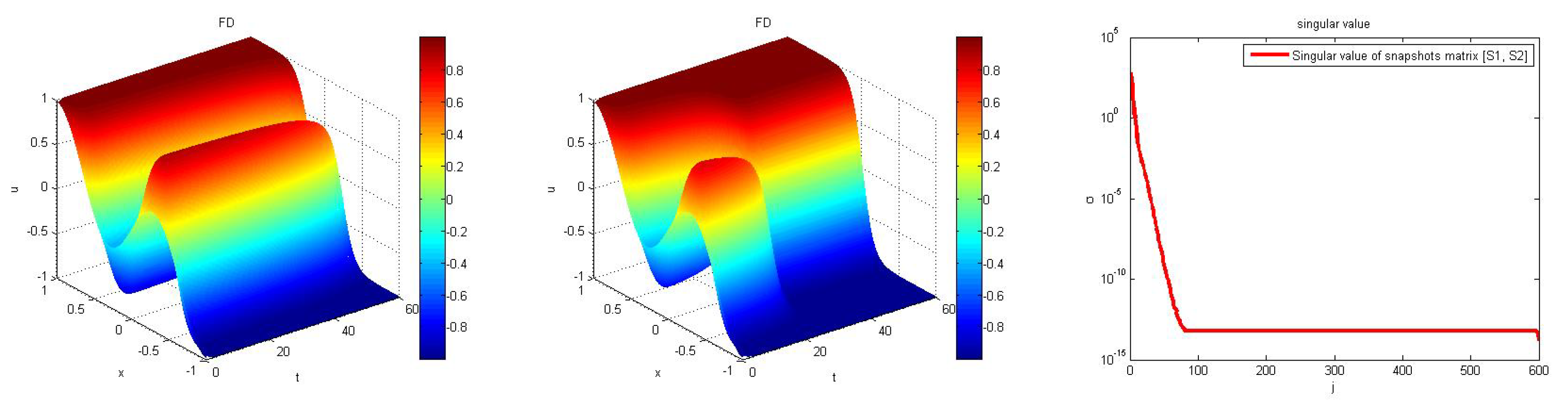
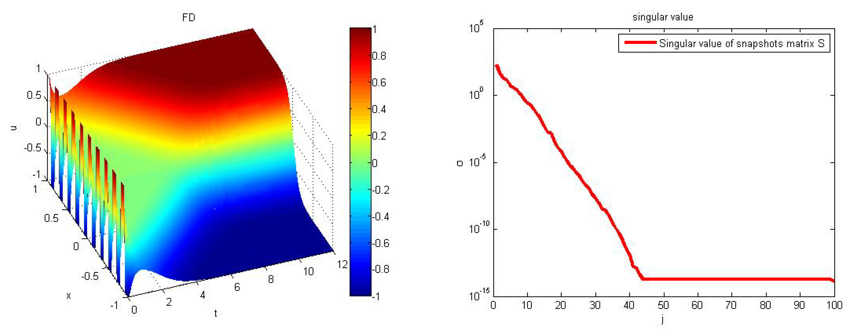
First, we selected wave crest $a=1$ and wave trough $b=-1$. We solved the numerical solution of the FD full system. When the time increases, the evolution of the Allen–Cahn equation still keeps the phase separation after long time calculation in the left plot of Figure 1. From the right plot of Figure 1, the decreasing of singular values of the snapshot matrix and then beginning to stabilize implies that solution information lies within a subspace whose dimension is significantly lower than the full dimension used in the discretization. That is, we can further reduce the dimensions of the full discretized system and still obtain accurate approximate solution.

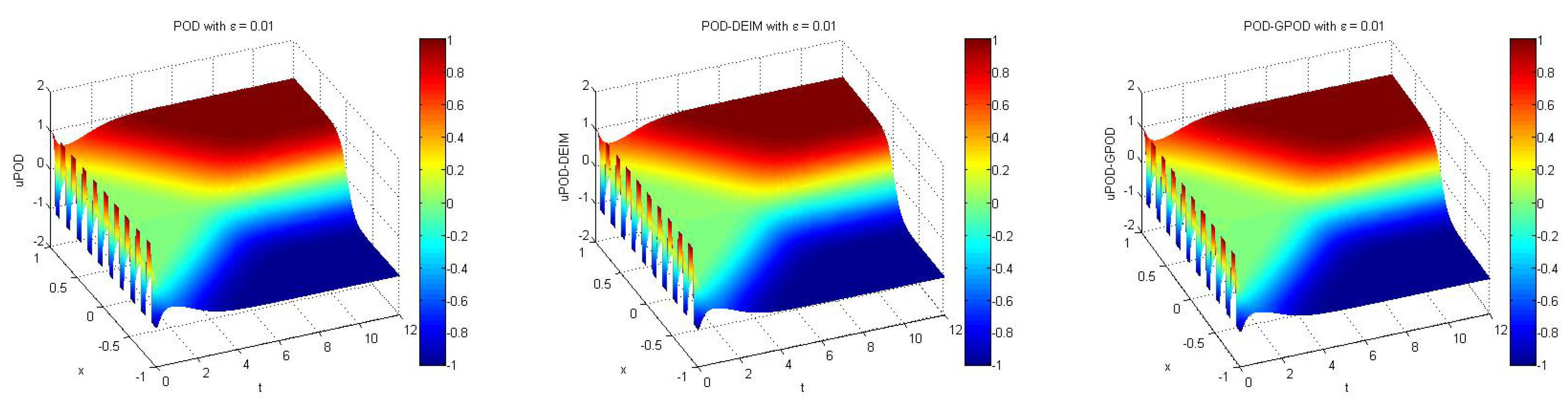
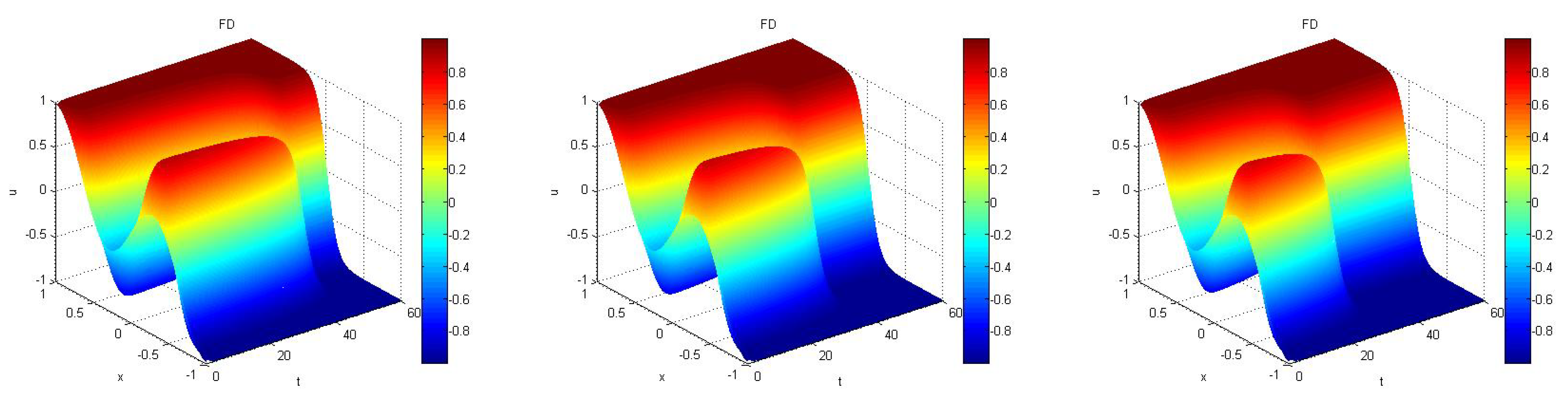
Next, we solved the numerical solution of the reduced system and used dimensions of POD basis $k=50$ and DEIM basis $m=60$. We obtained the approximate evolution of phase function of Allen–Cahn equation from POD, and POD-DEIM approaches for time $t=0$ to $t=12$ as shown in the first two plots of Figure 2. Finally, GPOD is used for reducing the complexity of the nonlinear term from the POD reduced system using a dimension of nonlinear basis m that is less than the number of selected rows q. The dimension of POD basis, nonlinear basis, and the number of selected rows in this numerical test are $k=50,m=60,$ and $q=90,$ respectively. We obtained the evolution of the phase function of Allen–Cahn equation by using POD-GPOD method for time $t=0$ to $t=12$ as shown in the last plot of Figure 2. Notice that the approximations from both POD-DEIM and POD-GPOD seem to be visually indistinguishable from the original solution. More details on errors are given in

Table 2. [Test 1] Runtime and error of the POD reduced system.

POD Basis (k)	Error	Runtime (Scaled %)
10	$1.0178\times {10}^{-3}$	20.93%
20	$1.2202\times {10}^{-7}$	21.14%
30	$4.9045\times {10}^{-11}$	21.63%
40	$7.2924\times {10}^{-14}$	22.25%
50	$7.3258\times {10}^{-14}$	22.61%
60	$7.3410\times {10}^{-14}$	24.46%
70	$7.3256\times {10}^{-14}$	31.61%
Full (100)	-	100%

and Figure 3.

The runtime and error from (21) are computed for POD-reduced system as shown in Table 2 and for POD-DEIM and POD-GPOD reduced systems as shown in

Table 3. [Test 1] Runtime and error of the POD-DEIM reduced system (left table) and POD-GPOD reduced system (right table) with POD basis with dimension $k=50$.

DEIM	Error	Runtime	GPOD:		Error	Runtime
m		(Scaled %)	m	q		(Scaled %)
10	$4.3498\times {10}^{-3}$	2.51%	10	40	$2.5195\times {10}^{-3}$	5.49%
20	$7.4722\times {10}^{-4}$	3.10%	20	50	$1.9981\times {10}^{-4}$	5.53%
30	$4.3472\times {10}^{-6}$	3.19%	30	60	$1.0603\times {10}^{-7}$	5.92%
40	$7.8929\times {10}^{-10}$	4.28%	40	70	$1.7405\times {10}^{-11}$	5.98%
50	$1.7124\times {10}^{-10}$	4.61%	50	80	$1.2332\times {10}^{-11}$	6.19%
60	$2.4349\times {10}^{-11}$	4.54%	60	90	$3.8857\times {10}^{-12}$	6.31%
70	$2.0649\times {10}^{-11}$	4.88%	70	100	$1.2603\times {10}^{-13}$	6.57%
Full	-	100%	Full	-	-	100%

for different dimension m of nonlinear basis, and number of selected rows q.

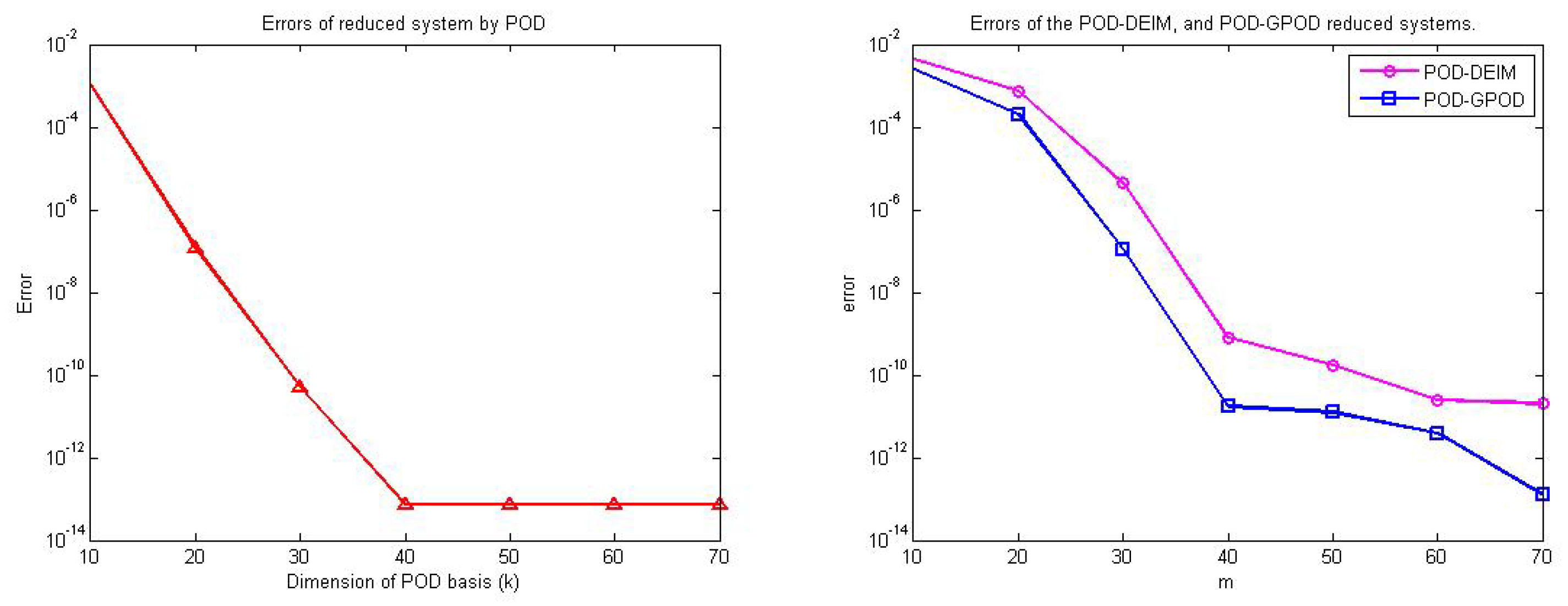
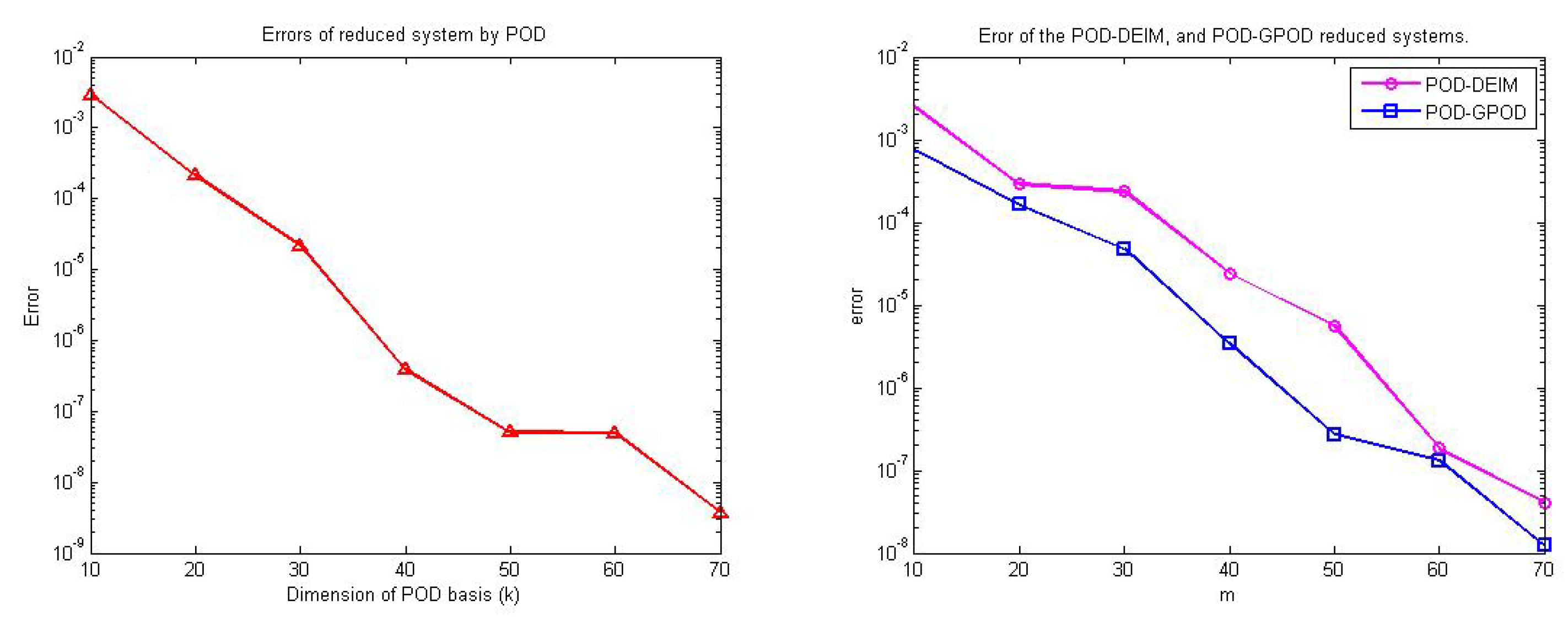
It can be observed in Figure 3 that the error decreases as the dimension of POD increases as also shown in Table 2. For a fixed POD dimension of $k=50,$ the error of POD-DEIM reduced system can be reduced by increasing the dimension of DEIM basis as shown in Table 3 and Figure 3. Similarly for POD-GPOD reduced system, when POD dimension is fixed to be $k=50$, the error can be decreased by increasing both the dimension of nonlinear basis and the number of selected rows as shown in Table 3. From Figure 3 and Table 3, for each m, the error of POD-GPOD approach is clearly smaller than the error of POD-DEIM approach.

Note that, from Figure 3, although the accuracy of the POD approach is higher (less error) than the POD-DEIM and POD-GPOD approaches, the reduction of the simulation time seems to be far less than these last two approaches, as shown in Table 2 and Table 3. To compare the speedup of the reduced order approaches, the runtimes given in Table 2 and Table 3 are all scaled with the simulation time for the full-order system, which is considered to be 100%. From Table 2, the runtime of POD approach is shown to be approximately 20–30% of the original full order system, i.e., around 3.3–5 times faster than the full order system, when the POD dimensions $k=10,20,\dots ,70$ are used. From Table 3, the POD-DEIM approach used only 2.51–4.88% of the full order system’s runtime, i.e., roughly 20–40 time faster, when POD dimension $k=50$ with DEIM dimension $m=10,\dots ,70$ are used. For POD-GPOD approach, as shown in the second part of Table 3, the runtime is reduced to approximately 5.49–6.57% of the original system, i.e., roughly 15–19 times faster than the original system. This shows that DEIM and GPOD techniques can significantly speed-up the simulation time of POD approach with small trade-off on accuracy. Notice that POD-DEIM approach provides the fastest speedup, but it has slightly less accuracy than the others. As a result, the POD-GPOD approach is shown to balance between the accuracy and the computational speedup.

In the next two numerical experiments, we will consider Allen–Cahn equation with parameter variation for different initial conditions and boundary conditions.

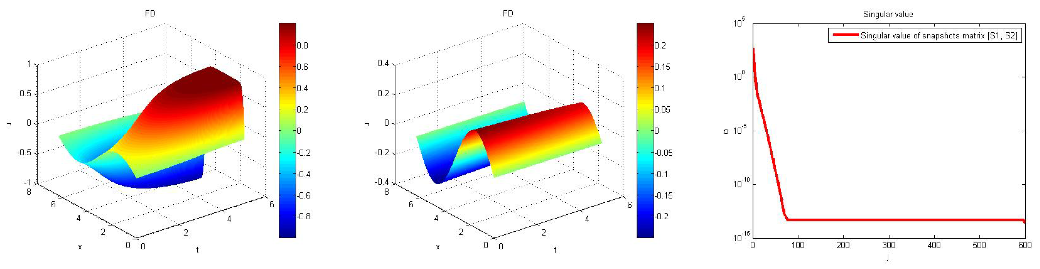
4.2. Numerical Test 2 (Parameter Variation): Homogeneous Boundary Conditions

The goal of this section is to construct reduced systems that have different values of a given parameter by using one basis set for each POD, DEIM, and GPOD. We consider Allen–Cahn Equation (1) with $\Omega =[\frac{2\pi }{n},2\pi ],$$n\in {\mathbb{Z}}^{+},$$n>1,$ the initial condition: $u(x,0)=0.25sin\left(x\right)$, and the homogeneous boundary conditions: $u(0,t)=0,u(2\pi ,t)=0,t>0$. In our numerical tests, the number of internal point is $n=600$ in $[2\pi ,\frac{2\pi }{n}]$, the number of time steps is $n_t=700$ on $[0,5]$ and $ϵ=0.01$. We used a space step-size is $\Delta x=\frac{2\pi }{n-1}$, time step-size is $\Delta t=\frac{5}{n_t-1}$ and the basis sets used in POD and DEIM approximations were constructed from $n_s=700$ snapshots.

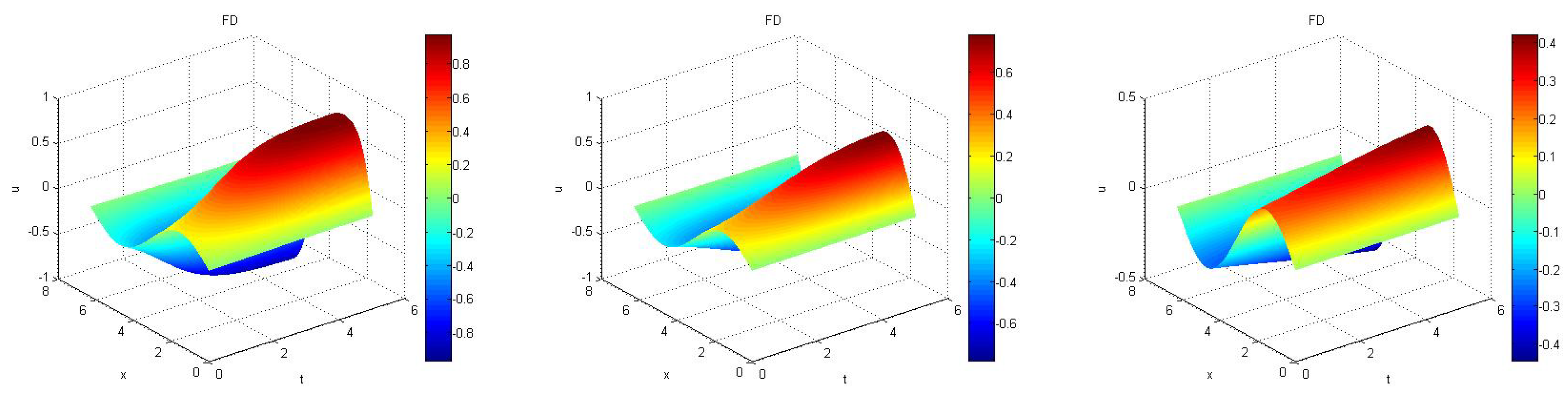
We used snapshots from the full systems with $ϵ=0.01$ and $ϵ=0.99$, as shown in Figure 4, respectively, to construct snapshot matrices ${\mathbf{S}}_1$, ${\mathbf{F}}_1$ and ${\mathbf{S}}_2$, ${\mathbf{F}}_2$. These snapshot matrices were used to construct basis sets for constructing reduced models with different parameter values $ϵ,$ i.e., $ϵ=0.2,0.5,0.8$ as shown in Figure 5. The singular values corresponding to the combined snapshot matrix $[{\mathbf{S}}_1,{\mathbf{S}}_2]$, which is used for computing POD basis, is shown in the last plot of Figure 4. The combined nonlinear snapshot matrix $[{\mathbf{F}}_1,{\mathbf{F}}_1]$ is used for constructing the basis for DEIM and GPOD approximations. Notice from the plots in Figure 4 and Figure 5 that the behaviors of the solutions are clearly different as the value of parameter $ϵ$ changes.

In

Table 4. [Test 2] Average runtime and average error of the POD reduced systems with parameter values $ϵ=0.2,0.5$ and $0.8$.

POD Basis (k)	Average Error	Average Runtime (Scaled %)
10	$2.9347\times {10}^{-3}$	39.37%
20	$2.1171\times {10}^{-4}$	41.61%
30	$2.1341\times {10}^{-5}$	43.69%
40	$3.8210\times {10}^{-7}$	46.12%
50	$5.0148\times {10}^{-8}$	46.79%
60	$4.9060\times {10}^{-8}$	46.87%
70	$3.7179\times {10}^{-9}$	46.91%
Full (100)	-	100%

and

Table 5. [Test 2] Average runtime and average error of the POD-DEIM and POD-GPOD reduced systems with various parameter values and POD basis with dimension $k=50$.

DEIM	Average Error	Avg Runtime	GPOD		Average Error	Avg Runtime
m		(Scaled %)	m	q		(Scaled %)
10	$2.4654\times {10}^{-3}$	0.19%	10	40	$7.6060\times {10}^{-4}$	0.39%
20	$2.8762\times {10}^{-4}$	0.20%	20	50	$1.6507\times {10}^{-4}$	0.40%
30	$2.3596\times {10}^{-4}$	0.22%	30	60	$4.7335\times {10}^{-5}$	0.40%
40	$2.3799\times {10}^{-5}$	0.25%	40	70	$3.3937\times {10}^{-6}$	0.40%
50	$5.6333\times {10}^{-6}$	0.28%	50	80	$2.7384\times {10}^{-7}$	0.41%
60	$1.8494\times {10}^{-7}$	0.29%	60	90	$1.3214\times {10}^{-7}$	0.42%
70	$4.0323\times {10}^{-8}$	0.32%	70	100	$1.2307\times {10}^{-8}$	0.42%
Full	-	100%	Full		-	100%

, the average of errors from (21) is given for POD, POD-DEIM, and POD-GPOD approaches with parameter variation $ϵ=0.2,$$0.5,$ and $0.8$. The corresponding average runtimes given in these tables are scaled with the runtime of the full order system, whose average runtime is considered to be 100%. Note that in Table 5, the dimension k is fixed to be 50 with different dimension m of nonlinear basis and different dimension q of selected rows.

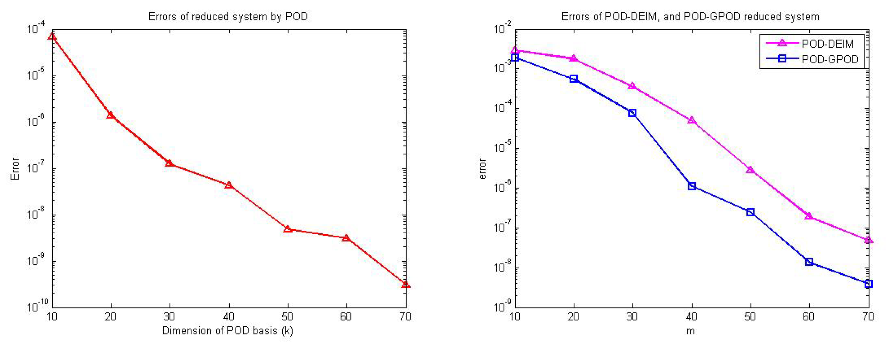
It can be observed that the decrease of the average error in Figure 6 corresponds to the increase of dimension of POD basis, as also shown in Table 4. At a fixed POD dimension of $k=50,$ the decrease of the average error corresponds to the increase of dimension of DEIM basis, as also shown in Table 5. Similarly, at a fixed POD dimension of $k=50,$ the decrease of the average error corresponds to the increase of both dimension of nonlinear basis and the number of selected rows in POD-GPOD approach. In Figure 6, the average error for the POD-GPOD reduced system is decreased more than the average error from the POD-DEIM reduced system. The average runtime of the reduced systems by POD approach was ranging between 39.37% to 46.91% of the average runtime of the full-order system, which is roughly 2.1–2.5 times speedup as shown in Table 4.

The average runtime in Table 4 shows that POD approach can speedup the simulation of the full-order model to roughly 2.1–2.5 times faster (using 39.37% to 46.91% of the average runtime for the full-order system). In Table 5, the POD-DEIM approach and POD-GPOD approach are shown to give around 300–500 times and 240–255 times, respectively, for the speedups. Although GPOD seems to use more simulation time than DEIM, it has already reduced the runtime of the full-order system (more than 200 time speedup) and, more importantly, it can provide approximation with less error than DEIM around one order of magnitude when the dimension $m\le 50$.

Table 6. [Test 2] The ratio of the average runtime of these systems to the runtime of the full discretized system with parameter values $ϵ=0.2,$$0.5,$ and $0.8$, using $k=50,$$m=40$ and $q=70$.

System	Average Error	Ratio of Average Runtime
The full discretized system	-	1
The POD reduced system	$\mathcal{O}\left({10}^{-8}\right)$	$1/2.1$
The POD-DEIM reduced system	$\mathcal{O}\left({10}^{-5}\right)$	$1/411$
The POD-GPOD reduced system	$\mathcal{O}\left({10}^{-6}\right)$	$1/254$

summarizes the accuracy and the scaled average computational time of the reduced systems when compared with the full-order system (the runtime of full-order system is normalized to be one), for a special case fixed dimensions $k=50$, $m=40$, and $q=70$.

4.3. Numerical Test 3 (Parameter Variation): Non-Homogeneous Boundary Conditions

This section considers parametrized Allen–Cahn Equation (1) with non-homogeneous boundary conditions. We used $\Omega =[-1,1]$, with the initial condition:

$u(x,0)=0.53x+0.47sin\left(1.5\pi x\right)$, and the non-homogeneous boundary conditions:

$u(-1,t)=-1,u(1,t)=1,t>0$. In this numerical tests, the number of internal points is $n=600$ in $[-1,1]$, the number of time steps is $n_t=700$ on $[0,60]$ and $ϵ=0.01$. We used a space step-size is $\Delta x=\frac{2}{n-1}$, time step-size is $\Delta t=\frac{60}{n_t-1}$. The value of parameter $ϵ$ is varying in this numerical test.

We used snapshots from the full systems with $ϵ=0.011$ and $ϵ=0.009$ from time $t=0$ to $t=60$, as shown in Figure 7, to construct matrices of solution snapshots and nonlinear snapshots. The decay of singular values of the matrix of solution snapshots is shown in the last plot of Figure 7. These snapshot matrices were used to construct basis sets for constructing reduced models of full systems with different parameter values $ϵ,$ i.e., $ϵ=0.0095,0.01,0.0105,$ as shown in Figure 8. Notice from Figure 7 and Figure 8 that the behaviors of the solutions are clearly different as the parameter changes, i.e., as the value of parameter $ϵ$ gets bigger, the solution reaches the steady state faster.

In

Table 7. [Test 3] Average runtime and average error of the POD reduced systems with parameter values $ϵ=0.0105,$$0.01,$ and $0.0095,$

POD Basis (k)	Average Error	Average Runtime (Scaled %)
10	$6.9201\times {10}^{-5}$	29.681%
20	$1.3413\times {10}^{-6}$	31.566%
30	$1.2395\times {10}^{-7}$	32.366%
40	$4.2427\times {10}^{-8}$	32.369%
50	$4.7703\times {10}^{-9}$	32.957%
60	$3.0531\times {10}^{-9}$	32.959%
70	$3.0827\times {10}^{-10}$	34.155%
Full	-	100 %

and

Table 8. [Test 3] Average runtime and average error of the POD-DEIM reduced systems with with parameter values $ϵ=0.0105,0.01,$ and $0.0095$. The POD basis has dimension $k=50$ for both POD-DEIM and POD-GPOD approaches.

DEIM	Average Error	Avg Runtime	GPOD		Average Error	Avg Runtime
m		(Scaled %)	m	q		(Scaled %)
10	$2.8847\times {10}^{-3}$	0.140%	10	40	$1.8960\times {10}^{-3}$	0.347%
20	$1.7506\times {10}^{-3}$	0.140%	20	50	$5.4464\times {10}^{-4}$	0.352%
30	$3.5277\times {10}^{-4}$	0.145%	30	60	$7.5895\times {10}^{-5}$	0.361%
40	$4.8921\times {10}^{-5}$	0.151%	40	70	$1.1070\times {10}^{-6}$	0.369%
50	$2.8691\times {10}^{-6}$	0.191%	50	80	$2.4638\times {10}^{-7}$	0.379%
60	$1.9001\times {10}^{-7}$	0.203%	60	90	$1.3442\times {10}^{-8}$	0.392%
70	$4.7991\times {10}^{-8}$	0.214%	70	100	$3.8939\times {10}^{-9}$	0.409%
Full	-	100%	Full		-	100%

, we present average runtimes and average errors from the parameter variation using $ϵ=0.0105,$ $0.01,$ and $0.0095,$ for POD, POD-DEIM, and POD-GPOD approaches, respectively. We computed the runtime and error from (4.1).

Table 8 shows the average error of the POD-GPOD reduced systems with POD basis of dimension $k=50$, where m is the dimension of nonlinear basis, and q is the number of selected rows.

The results in this section illustrate the same trends as in the previous numerical tests. From Table 7 and Table 8, the POD approach is more accurate, but it is much less efficient in term of computational time than the POD-DEIM and POD-GPOD approaches. From Table 7, when the POD approach uses $k=50$, the average error is of order $\mathcal{O}\left({10}^{-9}\right)$ and the average runtime is shown to be 32.957% of the full-order system, which is approximately three times faster than the full-order system. From Table 8, when the POD-DEIM reduced system uses $k=50$ and $m=50$, the average error is of order $\mathcal{O}\left({10}^{-6}\right)$ and the average runtime is 0.191% of the full-order system, which is approximately 524 times faster than the full-order system. From Table 8, when the POD-GPOD reduced system uses $k=50$, $m=50$ and $q=80$, the the average error is of order $\mathcal{O}\left({10}^{-7}\right)$ and the average runtime is 0.379% of the full-order system, which is approximately 264 times faster than the full-order system. Figure 9 shows that the reduced systems become more accurate as the dimension k for POD and dimension m for DEIM increase. As in the previous numerical test, the second plot in Figure 9 also demonstrates that the POD-GPOD reduced system is more accurate than the POD-DEIM reduced system for each fixed dimension m.

Table 9. [Test 3] The ratio of the average runtime of these systems to the runtime of the full discretized system, and average error of these systems with parameter values $ϵ=0.0105,0.01,$ and $0.0095$, using $k=50$, $m=60$, and $q=90$.

System	Average Error	Ratio of Average Runtime
The full discretized system	-	1
The POD reduced system	$\mathcal{O}\left({10}^{-9}\right)$	$1/3.0$
The POD-DEIM reduced system	$\mathcal{O}\left({10}^{-7}\right)$	$1/534$
The POD-GPOD reduced system	$\mathcal{O}\left({10}^{-8}\right)$	$1/261$

summarizes the accuracy and the scaled computational time of the reduced systems when compared with the full-order system. In Table 9, the ratio of the average runtime of the full discretized system is normalized to be 1. It considers a special case fixed dimensions $k=50$, $m=60$, and $q=90$. These results demonstrate that GPOD can further improve the accuracy of the DEIM, while still substantially decrease the computational complexity of the nonlinear term of POD reduced system.

5. Conclusions

In this paper, we consider model reduction techniques for Allen–Cahn equation. We introduced a modification of DEIM that is based on the concept of GPOD, called POD-GPOD approach, which compromises between the accuracy of POD and computational efficiency of DEIM. We compared the POD-GPOD approach with the standard POD method and POD-DEIM method on the parametrized Allen–Cahn equation. From the numerical results, as expected, the POD reduced system is more accurate than the POD-DEIM reduced system. However, the POD-DEIM reduced system can be used to substantially reduced the computational complexity in the nonlinear terms, and therefore the runtime for solving is significantly less than the POD reduced system. We extend the POD-DEIM reduced system to the POD-GPOD reduced system by increasing the selected rows used in the nonlinear approximation to improve the accuracy. The POD-GPOD reduced system can further reduce the approximation error when compare with the POD-DEIM reduced system with a small increase in simulation time that is still much less than the one used in POD approach. Therefore, POD-GPOD approach is an efficient method that can balance between the accuracy and efficiency for parametrized nonlinear model reduction. This approach can also readily be applied to other nonlinear dynamical systems and it is expected to outperform the standard POD approach in term of simulation time and outperform POD-DEIM approach in term of accuracy.

References

1. Allen, S.M.; Cahn, J.W. A microscopic theory for antiphase boundary motion and its application to antiphase domain coarsening. Acta Metall. 1979, 27, 1085–1095. [Google Scholar] [CrossRef]
2. Beneš, M.; Chalupeckỳ, V.; Mikula, K. Geometrical image segmentation by the Allen–Cahn equation. Appl. Numer. Math. 2004, 51, 187–205. [Google Scholar] [CrossRef]
3. Dobrosotskaya, J.A.; Bertozzi, A.L. A wavelet-Laplace variational technique for image deconvolution and inpainting. IEEE Trans. Image Process. 2008, 17, 657–663. [Google Scholar] [CrossRef]
4. Wheeler, A.A.; Boettinger, W.J.; McFadden, G.B. Phase-field model for isothermal phase transitions in binary alloys. Phys. Rev. A 1992, 45, 7424–7439. [Google Scholar] [CrossRef] [PubMed]
5. Feng, X.; Prohl, A. Numerical analysis of the Allen–Cahn equation and approximation for mean curvature flows. Numer. Math. 2003, 94, 33–65. [Google Scholar] [CrossRef]
6. Chen, L.Q. Phase-field models for microstructure evolution. Annu. Rev. Mater. Res. 2002, 32, 113–140. [Google Scholar] [CrossRef] [Green Version]
7. Mehrmann, V.; Stykel, T. Balanced truncation model reduction for large-scale systems in descriptor form. In Dimension Reduction of Large-Scale Systems; Springer: Berlin/Heidelberg, Germany, 2005; pp. 83–115. [Google Scholar]
8. Freund, R.W. Krylov-subspace methods for reduced-order modeling in circuit simulation. J. Comput. Appl. Math. 2000, 123, 395–421. [Google Scholar] [CrossRef] [Green Version]
9. Amsallem, D.; Farhat, C. Stabilization of projection-based reduced-order models. Int. J. Numer. Methods Eng. 2012, 91, 358–377. [Google Scholar] [CrossRef]
10. Daniel, L.; Siong, O.C.; Chay, L.S.; Lee, K.H.; White, J. A multiparameter moment-matching model-reduction approach for generating geometrically parameterized interconnect performance models. IEEE Trans. Comput. Aided Des. Integr. Circuits Syst. 2004, 23, 678–693. [Google Scholar] [CrossRef]
11. Lumley, J. The Structure of Inhomogeneous Turbulence in Atmospheric Turbulence and Radio Wave Propagation; Yaglom, A.M., Tatarski, V.I., Eds.; Atmospheric Turbulence and Wave Propagation: Moscow, Russia, 1967. [Google Scholar]
12. Loève, M. Probability Theory; Foundations, Random Sequences; D. Van Nostrand Company: New York, NY, USA, 1955. [Google Scholar]
13. Hotelling, H. Analysis of a complex of statistical variables into principal components. J. Educ. Psychol. 1933, 24, 417. [Google Scholar] [CrossRef]
14. Rathinam, M.; Petzold, L.R. A New Look at Proper Orthogonal Decomposition. SIAM J. Numer. Anal. 2003, 41, 1893–1925. [Google Scholar] [CrossRef]
15. Prajna, S. POD Model Reduction with Stability Guarantee. In Proceedings of the 42nd IEEE International Conference on Decision and Control, Maui, HI, USA, 9–12 December 2003. [Google Scholar]
16. Rosenfeld, A.; Kak, A.C. Digital Picture Processing; Academic Press: Cambridge, MA, USA, 1982. [Google Scholar]
17. Algazi, V.R.; Sakrison, D.J. On the optimality of the Karhunen-Loève expansion. IEEE Trans. Inf. Theory 1969, 15, 319–320. [Google Scholar] [CrossRef]
18. Holmes, P.; Lumley, J.L.; Berkooz, G. Turbulence, Coherent Structures, Dynamical Systems and Symmetry; Cambridge University Press: Cambridge, UK, 1998. [Google Scholar]
19. Glavaški, S.; Marsden, J.E.; Murray, R.M. Model reduction, centering, and the Karhunen-Loeve expansion. In Proceedings of the 37th IEEE Conference on Decision and Control, Tampa, FL, USA, 18 December 1998. [Google Scholar]
20. Parrilo, P.A.; Lall, S.; Paganini, F.; Verghese, G.C.; Lesieutre, B.C.; Marsden, J.E. Model reduction for analysis of cascading failures in power systems. In Proceedings of the 1999 American Control Conference, San Diego, CA, USA, 2–4 June 1999. [Google Scholar]
21. Shvartsman, S.; Kevrekidis, I. Low-dimensional approximation and control of periodic solutions in spatially extended systems. Phys. Rev. E 1998, 58, 361. [Google Scholar] [CrossRef]
22. Shvartsman, S.; Theodoropoulos, C.; Rico-Martınez, R.; Kevrekidis, I.; Titi, E.; Mountziaris, T. Order reduction for nonlinear dynamic models of distributed reacting systems. J. Process Control 2000, 10, 177–184. [Google Scholar] [CrossRef]
23. Noor, A.K.; Peters, J.M. Reduced basis technique for nonlinear analysis of structures. AIAA J. 1980, 18, 455–462. [Google Scholar] [CrossRef]
24. Peterson, J.S. The reduced basis method for incompressible viscous flow calculations. SIAM J. Sci. Stat. Comput. 1989, 10, 777–786. [Google Scholar] [CrossRef]
25. Ito, K.; Ravindran, S. A reduced-order method for simulation and control of fluid flows. J. Comput. Phys. 1998, 143, 403–425. [Google Scholar] [CrossRef] [Green Version]
26. Gunzburger, M.D.; Peterson, J.S.; Shadid, J.N. Reduced-order modeling of time-dependent PDEs with multiple parameters in the boundary data. Comput. Methods Appl. Mech. Eng. 2007, 196, 1030–1047. [Google Scholar] [CrossRef]
27. Carlberg, K.; Farhat, C. A compact proper orthogonal decomposition basis for optimization-oriented reduced-order models. AIAA Pap. 2008, 5964, 10–12. [Google Scholar]
28. Carlberg, K.; Farhat, C. A low-cost, goal-oriented ‘compact proper orthogonal decomposition’ basis for model reduction of static systems. Int. J. Numer. Methods Eng. 2011, 86, 381–402. [Google Scholar] [CrossRef]
29. Narasingam, A.; Siddhamshetty, P.; Sang-Il Kwon, J. Temporal clustering for order reduction of nonlinear parabolic PDE systems with time-dependent spatial domains: Application to a hydraulic fracturing process. AIChE J. 2017, 63, 3818–3831. [Google Scholar] [CrossRef]
30. Varshney, A.; Pitchaiah, S.; Armaou, A. Feedback control of dissipative PDE systems using adaptive model reduction. AIChE J. 2009, 55, 906–918. [Google Scholar] [CrossRef]
31. Pourkargar, D.B.; Armaou, A. Modification to adaptive model reduction for regulation of distributed parameter systems with fast transients. AIChE J. 2013, 59, 4595–4611. [Google Scholar] [CrossRef]
32. Sidhu, H.S.; Narasingam, A.; Siddhamshetty, P.; Kwon, J.S.I. Model order reduction of nonlinear parabolic PDE systems with moving boundaries using sparse proper orthogonal decomposition: Application to hydraulic fracturing. Comput. Chem. Eng. 2018, 112, 92–100. [Google Scholar] [CrossRef] [Green Version]
33. Chaturantabut, S.; Sorensen, D.C. Nonlinear Model Reduction via Discrete Empirical Interpolation. SIAM J. Sci. Comput. 2010, 32, 2737–2764. [Google Scholar] [CrossRef]
34. Barrault, M.; Maday, Y.; Nguyen, N.C.; Patera, A.T. An ‘empirical interpolation’ method: Application to efficient reduced-basis discretization of partial differential equations. Comptes Rendus Math. 2004, 339, 667–672. [Google Scholar] [CrossRef]
35. Peherstorfer, B.; Butnaru, D.; Willcox, K.; Bungartz, H.J. Localized discrete empirical interpolation method. SIAM J. Sci. Comput. 2014, 36, A168–A192. [Google Scholar] [CrossRef]
36. Carlberg, K.; Bou-Mosleh, C.; Farhat, C. Efficient non-linear model reduction via a least-squares Petrov–Galerkin projection and compressive tensor approximations. Int. J. Numer. Methods Eng. 2011, 86, 155–181. [Google Scholar] [CrossRef]
37. Nguyen, N.; Patera, A.; Peraire, J. A ‘best points’ interpolation method for efficient approximation of parametrized functions. Int. J. Numer. Methods Eng. 2008, 73, 521–543. [Google Scholar] [CrossRef]
38. Astrid, P.; Weiland, S.; Willcox, K.; Backx, T. Missing point estimation in models described by proper orthogonal decomposition. IEEE Trans. Autom. Control 2008, 53, 2237–2251. [Google Scholar] [CrossRef] [Green Version]
39. Ojo, S.O.; Grivet-Talocia, S.; Paggi, M. Model order reduction applied to heat conduction in photovoltaic modules. Compos. Struct. 2015, 119, 477–486. [Google Scholar] [CrossRef] [Green Version]
40. Ştefănescu, R.; Navon, I.M. POD/DEIM nonlinear model order reduction of an ADI implicit shallow water equations model. J. Comput. Phys. 2013, 237, 95–114. [Google Scholar] [CrossRef] [Green Version]
41. Xiao, D.; Fang, F.; Buchan, A.G.; Pain, C.C.; Navon, I.M.; Du, J.; Hu, G. Non-linear model reduction for the Navier–Stokes equations using residual DEIM method. J. Comput. Phys. 2014, 263, 1–18. [Google Scholar] [CrossRef] [Green Version]
42. Hinze, M.; Kunkel, M. Discrete empirical interpolation in POD model order reduction of drift-diffusion equations in electrical networks. In Scientific Computing in Electrical Engineering SCEE 2010; Springer: Berlin/Heidelberg, Germany, 2012; pp. 423–431. [Google Scholar]
43. Everson, R.; Sirovich, L. Karhunen-loeve procedure for gappy data. JOSA A 1995, 12, 1657–1664. [Google Scholar] [CrossRef] [Green Version]
44. Bui-Thanh, T.; Damodaran, M.; Willcox, K.E. Aerodynamic data reconstruction and inverse design using proper orthogonal decomposition. AIAA J. 2004, 42, 1505–1516. [Google Scholar] [CrossRef] [Green Version]
45. Bos, R.; Bombois, X.; Van den Hof, P. Accelerating large-scale non-linear models for monitoring and control using spatial and temporal correlations. In Proceedings of the 2004 American Control Conference, Boston, MA, USA, 30 June–2 July 2004; Volume 4, pp. 3705–3710. [Google Scholar]
46. Willcox, K. Unsteady flow sensing and estimation via the gappy proper orthogonal decomposition. Comput. Fluids 2006, 35, 208–226. [Google Scholar] [CrossRef] [Green Version]
47. Lee, K.; Mavris, D.N. A Unifying Least Squares Perspective for Gappy Proper Orthogonal Decomposition and Probabilistic Principal Component Analysis. In Proceedings of the 39th AIAA Fluid Dynamics Conference, San Antonio, TX, USA, 22–25 June 2009; p. 3899. [Google Scholar]
48. Murray, N.E.; Ukeiley, L.S. An application of Gappy POD. Exp. Fluids 2007, 42, 79–91. [Google Scholar] [CrossRef]
49. Volkwein, S. Proper Orthogonal Decomposition: Theory and Reduced-Order Modelling; Lecture Notes; University of Konstanz: Konstanz, Germnay, 2013. [Google Scholar]
50. Willcox, K.; Peraire, J. Balanced model reduction via the proper orthogonal decomposition. AIAA J. 2002, 40, 2323–2330. [Google Scholar] [CrossRef]
51. Chaturantabut, S. Dimension Reduction for Unsteady Nonlinear Partial Differential Equations via Empirical Interpolation Methods; ProQuest: Morrisville, NC, USA, 2009. [Google Scholar]
Figure 1. Solution of the FD full-order system for Allen–Cahn equation with ϵ = 0.01 and the corresponding singular values of the snapshot matrix S from SVD using POD basis.
Algorithms 13 00148 g001
Figure 2. [Test 1] Solution of the POD, POD-DEIM, and POD-GPOD reduced systems with ϵ = 0.01 (from left to right).
Algorithms 13 00148 g002
Figure 3. [Test 1] Error plot of the approximation the POD reduced system (left plot) and the POD-DEIM, and POD-GPOD reduced systems (right plot) with dimension of DEIM or nonlinear basis m.
Algorithms 13 00148 g003
Figure 4. [Test 2] Solution of the full discretized system with ϵ = 0.01 . The last plot shows the singular values of the snapshot matrix [ S 1 , S 2 ] from SVD using POD basis.
Algorithms 13 00148 g004
Figure 5. [Test 2] Solution of the full discretized system with ϵ = 0.2 , 0.5 , 0.8 (from left to right).
Algorithms 13 00148 g005
Figure 6. [Test 2] Average error plot of the approximation the POD, POD-DEIM, and POD-GPOD reduced systems with dimension of DEIM or nonlinear basis m.
Algorithms 13 00148 g006
Figure 7. [Test 3] Solution of the full discretized systems with ϵ = 0.009 and ϵ = 0.011 , and the corresponding singular values these snapshots (from left to right).
Algorithms 13 00148 g007
Figure 8. [Test 3] Solution of the full discretized systems with ϵ = 0.0095 , 0.01 , 0.0105 (from left to right).
Algorithms 13 00148 g008
Figure 9. [Test 3] Average error plot of the approximation from POD reduced systems with parameter values ϵ = 0.0105 0.01 , and 0.0095 using different dimensions of POD basis k (left) and from the POD-DEIM and POD-GPOD reduced systems with different dimensions of nonlinear basis m for a fixed POD dimension k = 50 (right).
Algorithms 13 00148 g009