Ensemble Deep Learning Models for Forecasting Cryptocurrency Time-Series

Abstract

Nowadays, cryptocurrency has infiltrated almost all financial transactions; thus, it is generally recognized as an alternative method for paying and exchanging currency. Cryptocurrency trade constitutes a constantly increasing financial market and a promising type of profitable investment; however, it is characterized by high volatility and strong fluctuations of prices over time. Therefore, the development of an intelligent forecasting model is considered essential for portfolio optimization and decision making. The main contribution of this research is the combination of three of the most widely employed ensemble learning strategies: ensemble-averaging, bagging and stacking with advanced deep learning models for forecasting major cryptocurrency hourly prices. The proposed ensemble models were evaluated utilizing state-of-the-art deep learning models as component learners, which were comprised by combinations of long short-term memory (LSTM), Bi-directional LSTM and convolutional layers. The ensemble models were evaluated on prediction of the cryptocurrency price on the following hour (regression) and also on the prediction if the price on the following hour will increase or decrease with respect to the current price (classification). Additionally, the reliability of each forecasting model and the efficiency of its predictions is evaluated by examining for autocorrelation of the errors. Our detailed experimental analysis indicates that ensemble learning and deep learning can be efficiently beneficial to each other, for developing strong, stable, and reliable forecasting models.

1. Introduction

The global financial crisis of 2007–2009 was the most severe crisis over the last few decades with, according to the National Bureau of Economic Research, a peak to trough contraction of 18 months. The consequences were severe in most aspects of life including economy (investment, productivity, jobs, and real income), social (inequality, poverty, and social tensions), leading in the long run to political instability and the need for further economic reforms. In an attempt to “think outside the box” and bypass the governments and financial institutions manipulation and control, Satoshi Nakamoto [1] proposed Bitcoin which is an electronic cash allowing online payments, where the double-spending problem was elegantly solved using a novel purely peer-to-peer decentralized blockchain along with a cryptographic hash function as a proof-of-work.

Nowadays, there are over 5000 cryptocurrencies available; however, when it comes to scientific research there are several issues to deal with. The large majority of these are relatively new, indicating that there is an insufficient amount of data for quantitative modeling or price forecasting. In the same manner, they are not highly ranked when it comes to market capitalization to be considered as market drivers. A third aspect which has not attracted attention in the literature is the separation of cryptocurrencies between mineable and non-mineable. Minable cryptocurrencies have several advantages i.e., the performance of different mineable coins can be monitored within the same blockchain which cannot be easily said for non-mineable coins, and they are community driven open source where different developers can contribute, ensuring the fact that a consensus has to be reached before any major update is done, in order to avoid splitting. Finally, when it comes to the top cryptocurrencies, it appears that mineable cryptocurrencies like Bitcoin (BTC) and Ethereum (ETH), recovered better the 2018 crash rather than Ripple (XRP) which is the highest ranked pre-mined coin. In addition, the non-mineable coins transactions are powered via a centralized blockchain, endangering price manipulation through inside trading, since the creators keep a given percentage to themselves, or through the use of pump and pull market mechanisms. Looking at the number one cryptocurrency exchange in the world, Coinmarketcap, by January 2020 at the time of writing there are only 31 mineable cryptocurrencies out of the first 100, ranked by market capitalization. The classical investing strategy in cryptocurrency market is the “buy, hold and sell” strategy, in which cryptocurrencies are bought with real money and held until reaching a higher price worth selling in order for an investor to make a profit. Obviously, a potential fractional change in the price of a cryptocurrency may gain opportunities for huge benefits or significant investment losses. Thus, the accurate prediction of cryptocurrency prices can potentially assist financial investors for making their proper investment policies by decreasing their risks. However, the accurate prediction of cryptocurrency prices is generally considered a significantly complex and challenging task, mainly due to its chaotic nature. This problem is traditionally addressed by the investor’s personal experience and consistent watching of exchanges prices. Recently, the utilization of intelligent decision systems based on complicated mathematical formulas and methods have been adopted for potentially assisting investors and portfolio optimization.

Let $y_1,y_2,\cdots ,y_n$ be the observations of a time series. Generally, a nonlinear regression model of order m is defined by

$$y_t=f(y_{t-1},y_{t-2},\cdots ,y_{t-m},\theta ),$$

(1)

where m values of $y_t$, $\theta$ is the parameter vector. After the model structure has been defined, function $f(·)$ can be determined by traditional time-series methods such as ARIMA (Auto-Regressive Integrated Moving Average) and GARCH-type models and their variations [2,3,4] or by machine learning methods such as Artificial Neural Networks (ANNs) [5,6]. However, both mentioned approaches fail to depict the stochastic and chaotic nature of cryptocurrency time-series and be successfully effective for accurate forecasting [7]. To this end, more sophisticated algorithmic approaches have to be applied such as deep learning and ensemble learning methods. From the perspective of developing strong forecasting models, deep learning and ensemble learning constitute two fundamental learning strategies. The former is based on neural networks architectures and it is able to achieve state-of-the-art accuracy by creating and exploiting new more valuable features by filtering out the noise of the input data; while the latter attempts to generate strong prediction models by exploiting multiple learners in order to reduce the bias or variance of error.

During the last few years, researchers paid special attention to the development of time-series forecasting models which exploit the advantages and benefits of deep learning techniques such as convolutional and long short-term memory (LSTM) layers. More specifically, Wen and Yuan [8] and Liu et al. [9] proposed Convolutional Neural Network (CNN) and LSTM prediction models for stock market forecasting. Along this line, Livieris et al. [10] and Pintelas et al. [11] proposed CNN-LSTM models with various architectures for efficiently forecasting gold and cryptocurrency time-series price and movement, reporting some interesting results. Nevertheless, although deep learning models are tailored to cope with temporal correlations and efficiently extract more valuable information from the training set, they failed to generate reliable forecasting models [7,11]; while in contrast ensemble learning models although they are an elegant solution to develop stable models and address the high variance of individual forecasting models, their performance heavily depends on the diversity and accuracy of the component learners. Therefore, a time-series prediction model, which exploits the benefits of both mentioned methodologies may significantly improve the prediction performance.

The main contribution of this research is the combination of ensemble learning strategies with advanced deep learning models for forecasting cryptocurrency hourly prices and movement. The proposed ensemble models utilize state-of-the-art deep learning models as component learners which are based on combinations of Long Short-Term Memory (LSTM), Bi-directional LSTM (BiLSTM) and convolutional layers. An extensive experimental analysis is performed considering both classification and regression problems, to evaluate the performance of averaging, bagging and stacking ensemble strategies. More analytically, all ensemble models are evaluated on prediction of the cryptocurrency price on the next hour (regression) and also on the prediction if the price on the following hour will increase or decrease with respect to the current price (classification). It is worth mentioning that the information of predicting the movement of a cryptocurrency is probably more significant that the prediction of the price for investors and financial institutions. Additionally, the efficiency of the predictions of each forecasting model is evaluated by examining for autocorrelation of the errors, which constitutes a significant reliability test of each model.

The remainder of the paper is organized as follows: Section 2 presents a brief review of state of the art deep learning methodologies for cryptocurrency forecasting. Section 3 presents the advanced deep learning models, while Section 4 presents the ensemble strategies utilized in our research. Section 5 presents our experimental methodology including the data preparation and preprocessing as well as the detailed experimental analysis, regarding the evaluation of ensemble of deep learning models. Section 6 discusses the obtained results and summarizes our findings. Finally, Section 7 presents our conclusions and presents some future directions.

2. Deep Learning in Cryptocurrency Forecasting: State-of-the-Art

Yiying and Yeze [12] focused on the price non-stationary dynamics of three cryptocurrencies Bitcoin, Etherium, and Ripple. Their approach aimed at identifying and understand the factors which influence the value formation of these digital currencies. Their collected data contained 1030 trading days regarding opening, high, low, and closing prices. They conducted an experimental analysis which revealed the efficiency of LSTM models over classical ANNs, indicating that LSTM models are more capable of exploiting information hidden in historical data. Additionally, the authors stated that probably the reason for the efficiency of LSTM networks is that they tend to depend more on short-term dynamics while ANNs tends to depend more on long-term history. Nevertheless, in case enough historical information is given, ANNs can achieve similar accuracy to LSTM networks.

Nakano et al. [13] examined the performance of ANNs for the prediction of Bitcoin intraday technical trading. The authors focused on identifying the key factors which affect the prediction performance for extracting useful trading signals of Bitcoin from its technical indicators. For this purposed, they conducted a series of experiments utilizing various ANN models with shallow and deep architectures and datasets structures The data utilized in their research regarded Bitcoin time-series return data at 15-min time intervals. Their experiments illustrated that the utilization of multiple technical indicators could possibly prevent the prediction model from overfitting of non-stationary financial data, which enhances trading performance. Moreover, they stated that their proposed methodology attained considerably better performance than the primitive technical trading and buy-and-hold strategies, under realistic assumptions of execution costs.

Mcnally et al. [14] utilized two deep learning models, namely a Bayesian-optimised Recurrent Neural Network and a LSTM network, for Bitcoin price prediction. The utilized data ranged from the August 2013 until July 2016, regarding open, high, low and close of Bitcoin prices as well as the block difficulty and hash rate. Their performance evaluation showed that the LSTM network demonstrated the best prediction accuracy, outperforming the other recurrent model as well as the classical statistical method ARIMA.

Shintate and Pichl [15] proposed a new trend prediction classification framework which is based on deep learning techniques. Their proposed framework utilized a metric learning-based method, called Random Sampling method, which measures the similarity between the training samples and the input patterns. They used high frequency data (1-min) ranged from June 2013 to March 2017 containing historical data from OkCoin Bitcoin market (Chinese Yuan Renminbi and US Dollars). The authors concluded that the profit rates based on utilized sampling method considerably outperformed those based on LSTM networks, confirming the superiority of the proposed framework. In contrast, these profit rates were lower than those obtained of the classical buy-and-hold strategy; thus they stated that it does not provide a basis for trading.

Miura et al. [16] attempted to analyze the high-frequency Bitcoin (1-min) time series utilizing machine learning and statistical forecasting models. Due to the large size of the data, they decided to aggregate the realized volatility values utilizing 3-h long intervals. Additionally, they pointed out that these values presented a weak correlation based on high-low price extent with the relative values of the 3-h interval. In their experimental analysis, they focused on evaluating various ANNs-type models, SVMs and Ridge Regression and the Heterogeneous Auto-Regressive Realized Volatility model. Their results demonstrated that Ridge Regression considerably presented the best performance while SVM exhibited poor performance.

Ji et al. [17] evaluated the prediction performance on Bitcoin price of various deep learning models such as LSTM networks, convolutional neural networks, deep neural networks, deep residual networks and their combinations. The data used in their research, contained 29 features of the Bitcoin blockchain from 2590 days (from 29 November 2011 to 31 December 2018). They conducted a detailed experimental procedure considering both classification and regression problems, where the former predicts whether or not the next day price will increase or decrease and the latter predicts the next day’s Bitcoin price. The numerical experiments illustrated that the deep neural DNN-based models performed the best for price ups-and-downs while the LSTM models slightly outperformed the rest of the models for forecasting Bitcoin’s price.

Kumar and Rath [18] focused on forecasting the trends of Etherium prices utilizing machine learning and deep learning methodologies. They conducted an experimental analysis and compared the prediction ability of LSTM neural networks and Multi-Layer perceptron (MLP). They utilized daily, hourly, and minute based data which were collected from the CoinMarket and CoinDesk repositories. Their evaluation results illustrated that LSTM marginally outperformed MLP but not considerably, although their training time was significantly high.

Pintelas et al. [7,11] conducted a detailed research, evaluating advanced deep learning models for predicting major cryptocurrency prices and movements. Additionally, they conducted a detailed discussion regarding the fundamental research questions: Can deep learning algorithms efficiently predict cryptocurrency prices? Are cryptocurrency prices a random walk process? Which is a proper validation method of cryptocurrency price prediction models? Their comprehensive experimental results revealed that even the LSTM-based and CNN-based models, which are generally preferable for time-series forecasting [8,9,10], were unable to generate efficient and reliable forecasting models. Moreover, the authors stated that cryptocurrency prices probably follow an almost random walk process while few hidden patterns may probably exist. Therefore, new sophisticated algorithmic approaches should be considered and explored for the development of a prediction model to make accurate and reliable forecasts.

In this work, we advocate combining the advantages of ensemble learning and deep learning for forecasting cryptocurrency prices and movement. Our research contribution aims on exploiting the ability of deep learning models to learn the internal representation of the cryptocurrency data and the effectiveness of ensemble learning for generating powerful forecasting models by exploiting multiple learners for reducing the bias or variance of error. Furthermore, similar to our previous research [7,11], we provide detailed performance evaluation for both regression and classification problems. To the best of our knowledge, this is the first research devoted to the adoption and combination of ensemble learning and deep learning for forecasting cryptocurrencies prices and movement.

3. Advanced Deep Learning Techniques

3.1. Long Short-Term Memory Neural Networks

Long Short-term memory (LSTM) [19] constitutes a special case of recurrent neural networks which were originally proposed to model both short-term and long-term dependencies [20,21,22]. The major novelty unit in a LSTM network is the memory block in the recurrent hidden layer which contains memory cells with self-connections memorizing the temporal state and adaptive gate units for controlling the information flow in the block. With the treatment of the hidden layer as a memory unit, LSTM can cope the correlation within time-series in both short and long term [23].

More analytically, the structure of the memory cell $c_t$ is composed by three gates: the input gate, the forget gate and the output gate. At every time step t, the input gate $i_t$ determines which information is added to the cell state $S_t$ (memory), the forget gate $f_t$ determines which information is thrown away from the cell state through the decision by a transformation function in the forget gate layer; while the output gate $o_t$ determines which information from the cell state will be used as output.

With the utilization of gates in each cell, data can be filtered, discarded or added. In this way, LSTM networks are capable of identifying both short and long term correlation features within time series. Additionally, it is worth mentioning that a significant advantage of the utilization of memory cells and adaptive gates which control information flow is that the vanishing gradient problem can be considerably addressed, which is crucial for the generalization performance of the network [20].

The simplest way to increase the depth and the capacity of LSTM networks is to stack LSTM layers together, in which the output of the $(L-1)$th LSTM layer at time t is treated as input of the Lth layer. Notice that this input-output connections are the only connections between the LSTM layers of the network. Based on the above formulation, the structure of the stacked LSTM can be describe as follows: Let $h_t^L$ and $h_t^{L-1}$ denote outputs in the Lth and $(L-1)$th layer, respectively. Each layer L produces a hidden state $h_t^L$ based on the current output of the previous layer $h_t^{L-1}$ and time $h_{t-1}^L$. More specifically, the forget gate $f_t^L$ of the L layer calculates the input for cell state $c_{t-1}^L$ by

$$f_t=\sigma \left(W_f^L[h_{t-1}^L,h_t^{L-1}]+b_f^L\right),$$

where $\sigma (·)$ is a sigmoid function while $W_f^L$ and $b_f$ are the weights matrix and bias vector of layer L regarding the forget gate, respectively. Subsequently, the input gate $i_t^L$ of the L layer computes the values to be added to the memory cell $c_t^L$ by

$$i_t^L=\sigma \left(W_i^L[h_{t-1}^L,h_t^{L-1}]+b_i^L\right),$$

where $W_i^L$ is the weights matrix of layer L regarding the input gate. Then, the output gate $o_t^L$ of the Lth layer filter the information and calculated the output value by

$$o_t^L=\sigma \left(W_o^L[h_{t-1}^L,h_t^{L-1}]+b_o^L\right),$$

where $W_f^o$ and $b_o$ are the weights matrix and bias vector of the output gate in the L layer, respectively. Finally, the output of the memory cell is computed by

$$h_t=o_t^L·tanh\left(c_t^L\right),$$

where · denotes the pointwise vector multiplication, tanh the hyperbolic tangent function and

$$\begin{array}{ccc}\hfill c_t^L& =& f_t^L·c_{t-1}^L+i_t^L·{\tilde{c}}_{t-1}^L,\hfill \\ \hfill {\tilde{c}}_t^L& =& tanh\left(W_{\tilde{c}}^L[h_{t-1}^L,h_t^{L-1}]+b_{\tilde{c}}^L\right).\hfill \end{array}$$

3.2. Bi-Directional Recurrent Neural Networks

Similar with the LSTM networks, one of the most efficient and widely utilized RNNs architectures are the Bi-directional Recurrent Neural Networks (BRNNs) [24]. In contrast with the LSTM, these networks are composed by two hidden layers, connected to input and output. The principle idea of BRNNs is that each training sequence is presented forwards and backwards into two separate recurrent networks [20]. More specifically, the first hidden layer possesses recurrent connections from the past time steps, while in the second one, the recurrent connections are reversed, transferring activation backwards along the sequence. Given the input and target sequences, the BRNN can be unfolded across time in order to be efficiently trained utilizing a classical backpropagation algorithm.

In fact, BRNN and LSTM are based on compatible techniques in which the former proposes the wiring of two hidden layers, which compose the network, while the latter proposes a new fundamental unit for composing the hidden layer.

Along this line, Bi-directional LSTM (BiLSTM) networks [25] were proposed in the literature, which incorporate two LSTM networks in the BRNN framework. More specifically, BiLSTM incorporates a forward LSTM layer and a backward LSTM layer in order to learn information from preceding and following tokens. In this way, both past and future contexts for a given time t are accessed, hence better prediction can be achieved by taking advantage of more sentence-level information.

In a bi-directional stacked LSTM network, the output of each feed-forward LSTM layer is the same as in the classical stacked LSTM layer and these layers are iterated from $t=1$ to T. In contrast, the output of each backward LSTM layer is iterated reversely, i.e., from $t=T$ to 1. Hence, at time t, the output of value ${\overleftarrow{h}}_t$ in backward LSTM layer L can be calculated as follows

$$\begin{array}{ccc}\hfill {\overleftarrow{f}}_t& =& \sigma \left(W_{\overleftarrow{f}}^L[h_{t-1}^L,h_t^{L-1}]+b_{\overleftarrow{f}}^L\right),\hfill \\ \hfill {\overleftarrow{i}}_t^L& =& \sigma \left(W_{\overleftarrow{i}}^L[h_{t-1}^L,h_t^{L-1}]+b_{\overleftarrow{i}}^L\right),\hfill \\ \hfill {\overleftarrow{o}}_t^L& =& \sigma \left(W_{\overleftarrow{o}}^L[h_{t-1}^L,h_t^{L-1}]+b_{\overleftarrow{o}}^L\right),\hfill \\ \hfill {\overleftarrow{c}}_t^L& =& {\overleftarrow{f}}_t^L·{\overleftarrow{c}}_{t-1}^L+{\overleftarrow{i}}_t^L·{\overleftarrow{\tilde{c}}}_{t-1}^L,\hfill \\ \hfill {\overleftarrow{\tilde{c}}}_t^L& =& tanh\left(W_{\overleftarrow{\tilde{c}}}^L[h_{t-1}^L,h_t^{L-1}]+b_{\overleftarrow{\tilde{c}}}^L\right),\hfill \\ \hfill {\overleftarrow{h}}_t& =& {\overleftarrow{o}}_t^L·tanh\left({\overleftarrow{c}}_t^L\right).\hfill \end{array}$$

Finally, the output of this BiLSTM architecture is given by

$$y_t=W\left[{\overrightarrow{h}}_t,{\overleftarrow{h}}_t\right]+b.$$

3.3. Convolutional Neural Networks

Convolutional Neural Network (CNN) models [26,27] were originally proposed for image recognition problems, achieving human level performance in many cases. CNNs have great potential to identify the complex patterns hidden in time series data. The advantage of the utilization of CNNs for time series is that they can efficiently extract knowledge and learn an internal representation from the raw time series data directly and they do not require special knowledge from the application domain to filter input features [10].

A typical CNN consists of two main components: In the first component, mathematical operations, called convolution and pooling, are utilized to develop features of the input data while in the second component, the generated features are used as input to a usually fully-connected neural network.

The convolutional layer constitutes the core of a CNN which systematically applies trained filters to input data for generating feature maps. Convolution can be considered as applying and sliding a one dimension (time) filter over the time series [28]. Moreover, since the output of a convolution is a new filtered time series, the application of several convolutions implies the generation of a multivariate times series whose dimension equals with the number of utilized filters in the layer. The rationale behind this strategy is that the application of several convolution leads to the generation of multiple discriminative features which usually improve the model’s performance. In practice, this kind of layer is proven to be very efficient and stacking different convolutional layers allows deeper layers to learn high-order or more abstract features and layers close to the input to learn low-level features.

Pooling layers were proposed to address the limitation that feature maps generated by the convolutional layers, record the precise position of features in the input. These layers aggregate over a sliding window over these feature maps, reducing their length, in order to attain some translation invariance of the trained features. More analytically, the feature maps obtained from the previous convolutional layer are pooled over temporal neighborhood separately by sum pooling function or by max pooling function in order to developed a new set of pooled feature maps. Notice that the output pooled feature maps constitute a filtered version of the features maps which are imported as inputs in the pooling layer [28]. This implies that small translations of the inputs of the CNN, which are usually detected by the convolutional layers, will become approximately invariant.

Finally, in addition to convolutional and pooling layers, some include batch normalization layers [29] and dropout layers [30] in order to accelerate the training process and reduce overfitting, respectively.

4. Ensemble Deep Learning Models

Ensemble learning has been proposed as an elegant solution to address the high variance of individual forecasting models and reduce the generalization error [31,32,33]. The basic principle behind any ensemble strategy is to weigh a number of models and combine their individual predictions for improving the forecasting performance; while the key point for the effectiveness of the ensemble is that its components should be characterized by accuracy and diversity in their predictions [34]. In general, the combination of multiple models predictions adds a bias which in turn counters the variance of a single trained model. Therefore, by reducing the variance in the predictions, the ensemble can perform better than any single best model.

In the literature, several strategies were proposed to design and develop ensemble of regression models. Next, we present three of the most efficient and widely employed strategies: ensemble-averaging, bagging, and stacking.

4.1. Ensemble-Averaging of Deep Learning Models

Ensemble-averaging [35] (or averaging) is the simplest combination strategy for exploiting the prediction of different regression models. It constitutes a commonly and widely utilized ensemble strategy of individual trained models in which their predictions are treated equally. More specifically, each forecasting model is individually trained and the ensemble-averaging strategy linearly combines all predictions by averaging them to develop the output. Figure 1 illustrates a high-level schematic representation of the ensemble-averaging of deep learning models.

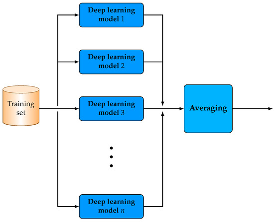
Figure 1. Ensemble-averaging of deep learning models.

Ensemble-averaging is based on the philosophy that its component models will not usually make the same error on new unseen data [36]. In this way, the ensemble model reduces the variance in the prediction, which results in better predictions compared to a single model. The advantages of this strategy are its simplicity of implementation and the exploitation of the diversity of errors of its component models without requiring any additional training on large quantities of the individual predictions.

4.2. Bagging Ensemble of Deep Learning Models

Bagging [33] is one the most widely used and successful ensemble strategies for improving the forecasting performance of unstable models. Its basic principle is the development of more diverse forecasting models by modifying the distribution of the training set based on a stochastic strategy. More specifically, it applies the same learning algorithm on different bootstrap samples of the original training set and the final output is produced via a simple averaging. An attractive property of the bagging strategy is that it reduces variance while simultaneously retains the bias which assists in avoiding overfitting [37,38]. Figure 2 demonstrates a high-level schematic representation of the bagging ensemble of n deep learning models.

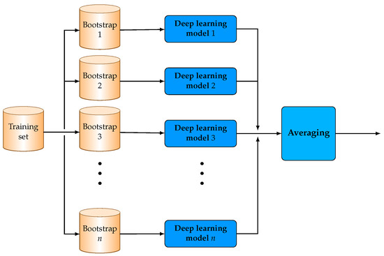
Figure 2. Bagging ensemble of deep learning models.

It is worth mentioning that bagging strategy is significantly useful for dealing with large and high-dimensional datasets where finding a single model which can exhibit good performance in one step is impossible due to the complexity and scale of the prediction problem.

4.3. Stacking Ensemble of Deep Learning Models

Stacked generalization or stacking [39] constitutes a more elegant and sophisticated approach for combining the prediction of different learning models. The motivation of this approach is based on the limitation of simple ensemble-average which is that each model is equally considered to the ensemble prediction, regardless of how well it performed. Instead, stacking induces a higher-level model for exploiting and combining the prediction of the ensemble’s component models. More specifically, the models which comprise the ensemble (Level-0 models) are individually trained using the same training set (Level-0 training set). Subsequently, a Level-1 training set is generated by the collected outputs of the component classifiers.

This dataset is utilized to train a single Level-1 model (meta-model) which ultimately determines how the outputs of the Level-0 models should be efficiently combined, to maximize the forecasting performance of the ensemble. Figure 3 illustrates the stacking of deep learning models.

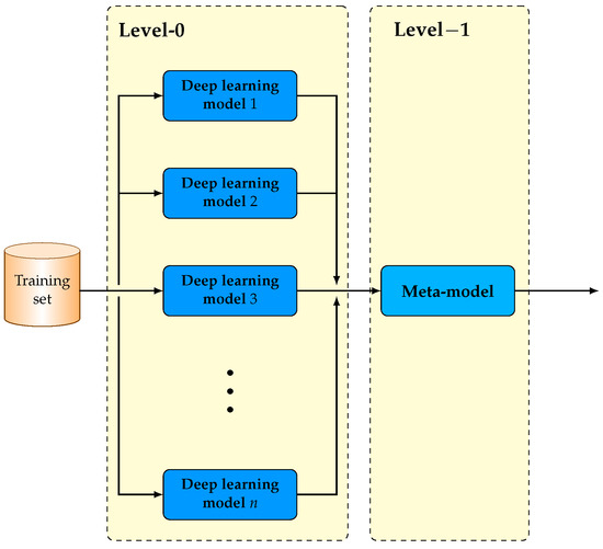
Figure 3. Stacking ensemble of deep learning models.

In general, stacked generalization works by deducing the biases of the individual learners with respect to the training set [33]. This deduction is performed by the meta-model. In other words, the meta-model is a special case of weighted-averaging, which utilizes the set of predictions as a context and conditionally decides to weight the input predictions, potentially resulting in better forecasting performance.

5. Numerical Experiments

In this section, we evaluate the performance of the three presented ensemble strategies which utilize advanced deep learning models as component learners. The implementation code was written in Python 3.4 while for all deep learning models Keras library [40] was utilized and Theano as back-end.

For the purpose of this research, we utilized data from 1 January 2018 to 31 August 2019 from the hourly price of the cryptocurrencies BTC, ETH and XRP. For evaluation purposes, the data were divided in training set and in testing set as in [7,11]. More specifically, the training set comprised data from 1 January 2018 to 28 February 2019 (10,177 datapoints), covering a wide range of long and short term trends while the testing set consisted of data from 1 March 2019 to 31 August 2019 (4415 datapoints) which ensured a substantial amount of unseen out-of-sample prices for testing.

Next, we concentrated on the experimental analysis to evaluate the presented ensemble strategies using the advanced deep learning models CNN-LSTM and CNN-BiLSTM as base learners. A detailed description of both component models is presented in Table 1. These models and their hyper-parameters were selected in previous research [7] after extensive experimentation, in which they exhibited the best performance on the utilized datasets. Both component models were trained for 50 epochs with Adaptive Moment Estimation (ADAM) algorithm [41] with a batch size equal to 512, using a mean-squared loss function. ADAM algorithm ensures that the learning steps, during the training process, are scale invariant relative to the parameter gradients.

Table 1. Parameter specification of two base learners.

Model	Description
CNN-LSTM	Convolutional layer with 32 filters of size (2, ) and padding = “same”.
	Convolutional layer with 64 filters of size (2, ) and padding = “same”.
	Max pooling layer with size (2, )
	LSTM layer with 70 units.
	Fully connected layer with 16 neurons.
	Output layer with 1 neuron.
CNN-BiLSTM	Convolutional layer with 64 filters of size (2, ) and padding = “same”.
	Convolutional layer with 128 filters of size (2, ) and padding = “same”.
	Max pooling layer with size (2, ).
	BiLSTM layer with $2\times 70$ units.
	Fully connected layer with 16 neurons.
	Output layer with 1 neuron.

The performance of all ensemble models was evaluated utilizing the performance metric: Root Mean Square Error (RMSE). Additionally, the classification accuracy of all ensemble deep models was measured, relative to the problem of predicting whether the cryptocurrency price would increase or decrease on the next day. More analytically, by analyzing a number of previous hourly prices, the model predicts the price on the following hour and also predicts if the price will increase or decrease, with respect to current cryptocurrency price. For this binary classification problem, three performance metrics were used: Accuracy (Acc), Area Under Curve (AUC) and $F_1$-score ($F_1$).

All ensemble models were evaluated using 7 and 11 component learners which reported the best overall performance. Notice that any attempt to increase the number of classifiers resulted to no improvement to the performance of each model. Moreover, stacking was evaluated using the most widely used state-of-the-art algorithms [42] as meta-learners: Support Vector Regression (SVR) [43], Linear Regression (LR) [44], k-Nearest Neighbor (kNN) [45] and Decision Tree Regression (DTR) [46]. For fairness and for performing an objective comparison, the hyper-parameters of all meta-learners were selected in order to maximize their experimental performance and are briefly presented in Table 2.

Table 2. Parameter specification of state-of-art algorithms used as meta-learners.

Model	Hyper-Parameters
DTR	Criterion = ’mse’,
	max depth = unlimited,
	min samples split = 2.
LR	No parameters specified.
SVR	Kernel = RBF,
	Regularization parameter $C=1.0$,
	$\mathrm{gamma}={10}^{-1}$.
kNN	Number of neighbors = 10,
	Euclidean distance.

Summarizing, we evaluate the performance of the following ensemble models:

• “Averaging${}_7$” and “Averaging${}_{11}$” stand for ensemble-averaging model utilizing 7 and 11 component learners, respectively.
• “Bagging${}_7$” and “Bagging${}_{11}$” stand for bagging ensemble model utilizing 7 and 11 component learners, respectively.
• “Stacking${}_7^{\left(\mathrm{DTR}\right)}$” and “Stacking${}_{11}^{\left(\mathrm{DTR}\right)}$” stand for stacking ensemble model utilizing 7 and 11 component learners, respectively and DTR model as meta-learner.
• “Stacking${}_7^{\left(\mathrm{LR}\right)}$” and “Stacking${}_{11}^{\left(\mathrm{LR}\right)}$” stand for stacking ensemble model utilizing 7 and 11 component learners, respectively and LR model as meta-learner.
• “Stacking${}_7^{\left(\mathrm{SVR}\right)}$” and “Stacking${}_{11}^{\left(\mathrm{SVR}\right)}$” stand for stacking ensemble model utilizing 7 and 11 component learners, respectively and SVR as meta-learner.
• “Stacking${}_7^{\left(k\mathrm{NN}\right)}$” and “Stacking${}_{11}^{\left(k\mathrm{NN}\right)}$” stand for stacking ensemble model utilizing 7 and 11 component learners, respectively and kNN as meta-learner.

Table 3 and Table 4 summarize the performance of all ensemble models using CNN-LSTM as base learner for $m=4$ and $m=9$, respectively. Stacking using LR as meta-learner exhibited the best regression performance, reporting the lowest RMSE score, for all cryptocurrencies. Notice that stacking${}_7^{\left(\mathrm{LR}\right)}$ and Stacking${}_{11}^{\left(\mathrm{LR}\right)}$ reported the same performance, which implies that the increment of component learners from 7 to 11 did not affect the regression performance of this ensemble algorithm. In contrast, stacking${}_7^{\left(\mathrm{LR}\right)}$ exhibited better classification performance than Stacking${}_{11}^{\left(\mathrm{LR}\right)}$, reporting higher accuracy, AUC and $F_1$-score. Additionally, the stacking ensemble reported the worst performance utilizing DTR and SVR as meta-learners among all ensemble models, also reporting worst performance than CNN-LSTM model; while the best classification performance was reported using kNN as meta-learner in almost all cases.

Table 3. Performance of ensemble models using convolutional neural network and long short-term memory (CNN-LSTM) as base learner for $m=4$.

Model		BTC				ETH				XRP
	RMSE	Acc	AUC	${\mathit{F}}_{\mathbf{1}}$	RMSE	Acc	AUC	${\mathit{F}}_{\mathbf{1}}$	RMSE	Acc	AUC	${\mathit{F}}_{\mathbf{1}}$
CNN-LSTM	0.0101	52.80%	0.521	0.530	0.0111	53.39%	0.533	0.525	0.0110	53.82%	0.510	0.530
Averaging${}_7$	0.0096	54.39%	0.543	0.536	0.0107	53.73%	0.539	0.536	0.0108	54.12%	0.552	0.536
Bagging${}_7$	0.0097	54.52%	0.549	0.545	0.0107	53.95%	0.541	0.530	0.0095	53.29%	0.560	0.483
Stacking${}_7^{\left(\mathrm{DTR}\right)}$	0.0168	49.96%	0.510	0.498	0.0230	50.13%	0.506	0.497	0.0230	49.67%	0.530	0.492
Stacking${}_7^{\left(\mathrm{LR}\right)}$	0.0085	52.57%	0.530	0.524	0.0093	52.44%	0.513	0.515	0.0095	52.32%	0.537	0.514
Stacking${}_7^{\left(\mathrm{SVR}\right)}$	0.0128	49.82%	0.523	0.497	0.0145	51.24%	0.501	0.508	0.0146	51.27%	0.515	0.508
Stacking${}_7^{\left(k\mathrm{NN}\right)}$	0.0113	52.64%	0.525	0.511	0.0126	52.85%	0.537	0.473	0.0101	52.87%	0.536	0.514
Averaging${}_{11}$	0.0096	54.16%	0.545	0.534	0.0107	53.77%	0.542	0.535	0.0107	54.12%	0.531	0.537
Bagging${}_{11}$	0.0098	54.31%	0.546	0.542	0.0107	53.95%	0.548	0.536	0.0094	54.32%	0.532	0.515
Stacking${}_{11}^{\left(\mathrm{DTR}\right)}$	0.0169	49.66%	0.510	0.495	0.0224	50.42%	0.512	0.500	0.0229	50.63%	0.519	0.501
Stacking${}_{11}^{\left(\mathrm{LR}\right)}$	0.0085	51.05%	0.529	0.475	0.0093	51.95%	0.514	0.514	0.0094	52.35%	0.529	0.512
Stacking${}_{11}^{\left(\mathrm{SVR}\right)}$	0.0128	50.03%	0.520	0.499	0.0145	51.10%	0.510	0.506	0.0145	51.11%	0.511	0.506
Stacking${}_{11}^{\left(k\mathrm{NN}\right)}$	0.0112	52.66%	0.526	0.511	0.0126	52.65%	0.538	0.481	0.0101	53.05%	0.530	0.512

Table 4. Performance of ensemble models using CNN-LSTM as base learner for $m=9$.

Model		BTC				ETH				XRP
	RMSE	Acc	AUC	${\mathit{F}}_{\mathbf{1}}$	RMSE	Acc	AUC	${\mathit{F}}_{\mathbf{1}}$	RMSE	Acc	AUC	${\mathit{F}}_{\mathbf{1}}$
CNN-LSTM	0.0124	51.19%	0.511	0.504	0.0140	53.49%	0.535	0.513	0.0140	53.43%	0.510	0.510
Averaging${}_7$	0.0122	54.12%	0.549	0.541	0.0138	53.86%	0.539	0.538	0.0138	53.94%	0.502	0.538
Bagging${}_7$	0.0123	54.29%	0.549	0.543	0.0132	54.05%	0.541	0.539	0.0093	52.97%	0.501	0.502
Stacking${}_7^{\left(\mathrm{DTR}\right)}$	0.0213	50.57%	0.510	0.504	0.0280	51.58%	0.509	0.511	0.0279	51.87%	0.514	0.514
Stacking${}_7^{\left(\mathrm{LR}\right)}$	0.0090	51.19%	0.530	0.503	0.0098	52.17%	0.525	0.503	0.0098	51.89%	0.524	0.506
Stacking${}_7^{\left(\mathrm{SVR}\right)}$	0.0168	50.54%	0.523	0.503	0.0203	51.94%	0.515	0.513	0.0203	51.86%	0.518	0.512
Stacking${}_7^{\left(k\mathrm{NN}\right)}$	0.0165	52.00%	0.525	0.509	0.0179	52.66%	0.526	0.487	0.0100	51.91%	0.521	0.522
Averaging${}_{11}$	0.0122	54.25%	0.545	0.542	0.0136	54.02%	0.542	0.540	0.0136	54.03%	0.501	0.539
Bagging${}_{11}$	0.0124	54.30%	0.555	0.542	0.0134	54.11%	0.541	0.540	0.0093	53.11%	0.502	0.509
Stacking${}_{11}^{\left(\mathrm{DTR}\right)}$	0.0209	50.43%	0.510	0.502	0.0271	51.69%	0.510	0.512	0.0274	51.85%	0.519	0.512
Stacking${}_{11}^{\left(\mathrm{LR}\right)}$	0.0087	50.99%	0.529	0.492	0.0095	52.43%	0.522	0.507	0.0096	52.11%	0.514	0.501
Stacking${}_{11}^{\left(\mathrm{SVR}\right)}$	0.0165	50.66%	0.520	0.504	0.0202	51.85%	0.512	0.512	0.0202	51.82%	0.517	0.511
Stacking${}_{11}^{\left(k\mathrm{NN}\right)}$	0.0165	52.13%	0.526	0.505	0.0179	52.19%	0.523	0.489	0.0100	52.49%	0.521	0.520

The average and bagging ensemble reported slightly better regression performance, compared to the single model CNN-LSTM. In contrast, both ensembles presented the best classification performance, considerably outperforming all other forecasting models, regarding all datasets. Moreover, the bagging ensemble reported the highest accuracy, AUC and $F_1$ in most cases, slightly outperforming the average-ensemble model. Finally, it is worth noticing that both the bagging and average-ensemble did not improve their performance when the number of component classifiers increased. for $m=4$ while for $m=9$ a slightly improvement in their performance was noticed.

Table 5 and Table 6 present the performance of all ensemble models utilizing CNN-BiLSTM as base learner for $m=4$ and $m=9$, respectively. Firstly, it is worth noticing that stacking model using LR as meta-learner exhibited the best regression performance, regarding to all cryptocurrencies. Stacking${}_7^{\left(\mathrm{LR}\right)}$ and Stacking${}_{11}^{\left(\mathrm{LR}\right)}$ presented almost identical RMSE score Moreover, stacking${}_7^{\left(\mathrm{LR}\right)}$ presented slightly higher accuracy, AUC and $F_1$-score than stacking${}_{11}^{\left(\mathrm{LR}\right)}$, for ETH and XRP datasets, while for BTC dataset Stacking${}_{11}^{\left(\mathrm{LR}\right)}$ reported slightly better classification performance. This implies that the increment of component learners from 7 to 11 did not considerably improved and affected the regression and classification performance of the stacking ensemble algorithm. Stacking ensemble reported the worst (highest) RMSE score utilizing DTR, SVR and kNN as meta-learners. It is also worth mentioning that it exhibited the worst performance among all ensemble models and also worst than that of the single model CNN-BiLSTM. However, stacking ensemble reported the highest classification performance using kNN as meta-learner. Additionally, it presented slightly better classification performance using DTR or SVR than LR as meta-learners for ETH and XRP datasets, while for BTC dataset it presented better performance using LR as meta-learner as meta-learner.

Table 5. Performance of ensemble models using CNN and bi-directional LSTM (CNN-BiLSTM) as base learner for $m=4$.

Model		BTC				ETH				XRP
	RMSE	Acc	AUC	${\mathit{F}}_{\mathbf{1}}$	RMSE	Acc	AUC	${\mathit{F}}_{\mathbf{1}}$	RMSE	Acc	AUC	${\mathit{F}}_{\mathbf{1}}$
CNN-BiLSTM	0.0107	53.93%	0.528	0.522	0.0116	53.56%	0.525	0.521	0.0099	53.72%	0.519	0.484
Averaging${}_7$	0.0104	54.15%	0.548	0.537	0.0114	53.87%	0.530	0.536	0.0096	54.73%	0.555	0.532
Bagging${}_7$	0.0104	54.62%	0.549	0.544	0.0114	53.88%	0.532	0.529	0.0096	55.42%	0.557	0.520
Stacking${}_7^{\left(\mathrm{DTR}\right)}$	0.0176	50.33%	0.498	0.503	0.0224	51.20%	0.501	0.509	0.0155	51.66%	0.510	0.515
Stacking${}_7^{\left(\mathrm{LR}\right)}$	0.0085	51.67%	0.527	0.494	0.0095	52.81%	0.536	0.517	0.0093	51.04%	0.541	0.498
Stacking${}_7^{\left(\mathrm{SVR}\right)}$	0.0085	51.67%	0.510	0.494	0.0159	51.99%	0.513	0.517	0.0118	51.14%	0.511	0.510
Stacking${}_7^{\left(k\mathrm{NN}\right)}$	0.0112	52.18%	0.526	0.519	0.0126	54.15%	0.544	0.503	0.0101	52.56%	0.536	0.510
Averaging${}_{11}$	0.0105	54.41%	0.546	0.543	0.0114	53.83%	0.531	0.538	0.0095	55.55%	0.525	0.547
Bagging${}_{11}$	0.0104	54.66%	0.548	0.541	0.0113	54.07%	0.532	0.529	0.0096	55.64%	0.524	0.530
Stacking${}_{11}^{\left(\mathrm{DTR}\right)}$	0.0178	50.22%	0.494	0.502	0.0226	51.11%	0.510	0.508	0.0157	51.61%	0.518	0.514
Stacking${}_{11}^{\left(\mathrm{LR}\right)}$	0.0085	51.72%	0.527	0.499	0.0095	51.69%	0.533	0.492	0.0092	50.42%	0.545	0.496
Stacking${}_{11}^{\left(\mathrm{SVR}\right)}$	0.0085	51.72%	0.512	0.499	0.0161	52.36%	0.512	0.521	0.0116	51.82%	0.512	0.517
Stacking${}_{11}^{\left(k\mathrm{NN}\right)}$	0.0112	52.34%	0.521	0.504	0.0126	54.14%	0.542	0.492	0.0101	52.53%	0.529	0.509

Table 6. Performance of ensemble models using convolutional neural network with CNN-BiLSTM as base learner for $m=9$.

Model		BTC				ETH				XRP
	RMSE	Acc	AUC	${\mathit{F}}_{\mathbf{1}}$	RMSE	Acc	AUC	${\mathit{F}}_{\mathbf{1}}$	RMSE	Acc	AUC	${\mathit{F}}_{\mathbf{1}}$
CNN-BiLSTM	0.0146	53.47%	0.529	0.526	0.0154	53.87%	0.531	0.529	0.0101	50.36%	0.506	0.394
Averaging${}_7$	0.0146	53.58%	0.547	0.535	0.0151	54.03%	0.540	0.539	0.0095	50.04%	0.537	0.428
Bagging${}_7$	0.0143	53.20%	0.541	0.528	0.0155	54.09%	0.540	0.539	0.0095	51.11%	0.540	0.417
Stacking${}_7^{\left(\mathrm{DTR}\right)}$	0.0233	50.84%	0.521	0.507	0.0324	52.23%	0.522	0.517	0.0149	52.19%	0.519	0.521
Stacking${}_7^{\left(\mathrm{LR}\right)}$	0.0091	52.30%	0.518	0.516	0.0105	52.26%	0.525	0.512	0.0093	50.10%	0.522	0.488
Stacking${}_7^{\left(\mathrm{SVR}\right)}$	0.0109	52.30%	0.517	0.516	0.0235	52.10%	0.513	0.514	0.0112	51.28%	0.518	0.512
Stacking${}_7^{\left(k\mathrm{NN}\right)}$	0.0166	52.00%	0.522	0.508	0.0142	51.91%	0.529	0.475	0.0101	52.50%	0.523	0.510
Averaging${}_{11}$	0.0144	53.53%	0.548	0.535	0.0151	54.02%	0.539	0.537	0.0093	50.22%	0.549	0.437
Bagging${}_{11}$	0.0143	53.32%	0.547	0.530	0.0155	54.20%	0.539	0.539	0.0093	51.15%	0.551	0.470
Stacking${}_{11}^{\left(\mathrm{DTR}\right)}$	0.0235	50.76%	0.513	0.506	0.0305	52.41%	0.513	0.520	0.0152	51.72%	0.522	0.516
Stacking${}_{11}^{\left(\mathrm{LR}\right)}$	0.0088	50.48%	0.527	0.489	0.0098	52.67%	0.524	0.515	0.0092	50.68%	0.529	0.505
Stacking${}_{11}^{\left(\mathrm{SVR}\right)}$	0.0108	50.48%	0.513	0.489	0.0235	52.12%	0.516	0.514	0.0110	51.68%	0.517	0.516
Stacking${}_{11}^{\left(k\mathrm{NN}\right)}$	0.0166	52.00%	0.526	0.496	0.0142	51.95%	0.517	0.475	0.0100	52.32%	0.526	0.505

Regarding the other two ensemble strategies, averaging and bagging, they exhibited slightly better regression performance compared to the single CNN-BiLSTM model. Nevertheless, both averaging and bagging reported the highest accuracy, AUC and $F_1$-score, which implies that they presented the best classification performance among all other models with bagging exhibiting slightly better classification performance. Furthermore, it is also worth mentioning that both ensembles slightly improved their performance in term of RMSE score and Accuracy, when the number of component classifiers increased from 7 to 11.

In the follow-up, we provided a deeper insight classification performance of the forecasting models by presenting the confusion matrices of averaging${}_{11}$, bagging${}_{11}$, stacking${}_7^{\left(\mathrm{LR}\right)}$ and stacking${}_{11}^{\left(k\mathrm{NN}\right)}$ for $m=4$, which exhibited the best overall performance. The use of the confusion matrix provides a compact and to the classification performance of each model, presenting complete information about mislabeled classes. Notice that each row of a confusion matrix represents the instances in an actual class while each column represents the instances in a predicted class. Additionally, both stacking ensembles utilizing DTR and SVM as meta-learners were excluded from the rest of our experimental analysis, since they presented the worst regression and classification performance, relative to all cryptocurrencies.

Table 7, Table 8 and Table 9 present the confusion matrices of the best identified ensemble models using CNN-LSTM as base learner, regarding BTC, ETH and XRP datasets, respectively. The confusion matrices for BTC and ETH revealed that stacking${}_7^{\left(\mathrm{LR}\right)}$ is biased, since most of the instances were misclassified as “Down”, meaning that this model was unable to identify possible hidden patterns despite the fact that it exhibited the best regression performance. On the other hand, bagging${}_{11}$ exhibited a balanced prediction distribution between “Down” or “Up” predictions, presenting its superiority over the rest forecasting models, followed by averaging${}_{11}$ and stacking${}_{11}^{\left(\mathrm{kNN}\right)}$. Regarding XRP dataset, bagging${}_{11}$ and stacking${}_{11}^{\left(\mathrm{kNN}\right)}$ presented the highest prediction accuracy and the best trade-off between true positive and true negative rate, meaning that these models may have identified some hidden patters.

Table 7. Confusion matrices of Averaging${}_{11}$, Bagging${}_{11}$, Stacking${}_7^{\left(\mathrm{LR}\right)}$ and Stacking${}_{11}^{\left(k\mathrm{NN}\right)}$ using CNN-LSTM as base model for Bitcoin (BTC) dataset.

Averaging${}_{11}$			Bagging${}_{11}$			Stacking${}_7^{\left(\mathbf{LR}\right)}$			Stacking${}_{11}^{\left(\mathit{k}\mathbf{NN}\right)}$
	Down	Up		Down	Up		Down	Up		Down	Up
Down	1244	850	Down	1064	1030	Down	1537	557	Down	1296	798
Up	1270	1050	Up	922	1398	Up	1562	758	Up	1315	1005

Table 8. Confusion matrices of Averaging${}_{11}$, Bagging${}_{11}$, Stacking${}_7^{\left(\mathrm{LR}\right)}$ and Stacking${}_{11}^{\left(k\mathrm{NN}\right)}$ using CNN-LSTM as base model for Etherium (ETH) dataset.

Averaging${}_{11}$			Bagging${}_{11}$			Stacking${}_7^{\left(\mathbf{LR}\right)}$			Stacking${}_{11}^{\left(\mathit{k}\mathbf{NN}\right)}$
	Down	Up		Down	Up		Down	Up		Down	Up
Down	1365	885	Down	1076	1174	Down	1666	584	Down	1353	897
Up	1208	955	Up	866	1297	Up	1593	570	Up	1203	960

Table 9. Confusion matrices of Averaging${}_{11}$, Bagging${}_{11}$, Stacking${}_7^{\left(\mathrm{LR}\right)}$ and Stacking${}_{11}^{\left(k\mathrm{NN}\right)}$ using CNN-LSTM as base model for Ripple (XRP) dataset.

Averaging${}_{11}$			Bagging${}_{11}$			Stacking${}_7^{\left(\mathbf{LR}\right)}$			Stacking${}_{11}^{\left(\mathit{k}\mathbf{NN}\right)}$
	Down	Up		Down	Up		Down	Up		Down	Up
Down	1575	739	Down	1314	1000	Down	1072	1242	Down	1214	1100
Up	1176	923	Up	984	1115	Up	815	1284	Up	991	1108

Table 10, Table 11 and Table 12 present the confusion matrices of averaging${}_{11}$, bagging${}_{11}$, stacking${}_7^{\left(\mathrm{LR}\right)}$ and Stacking${}_{11}^{\left(k\mathrm{NN}\right)}$ using CNN-BiLSTM as base learner, regarding BTC, ETH and XRP datasets, respectively. The confusion matrices for BTC dataset demonstrated that both average${}_{11}$ and bagging${}_{11}$ presented the best performance while stacking${}_7^{\left(\mathrm{LR}\right)}$ was biased, since most of the instances were misclassified as “Down”. Regarding ETH dataset, both average${}_{11}$ and bagging${}_{11}$ were considered biased since most “Up” instances were misclassified as “Down”. In contrast, both stacking ensembles presented the best performance, with stacking${}_{11}^{\left(k\mathrm{NN}\right)}$ reporting slightly considerably better trade-off between sensitivity and specificity. Regarding XRP dataset, bagging${}_{11}$ presented the highest prediction accuracy and the best trade-off between true positive and true negative rate, closely followed by stacking${}_{11}^{\left(\mathrm{kNN}\right)}$.

Table 10. Confusion matrices of Averaging${}_{11}$, Bagging${}_{11}$, Stacking${}_7^{\left(\mathrm{LR}\right)}$ and Stacking${}_{11}^{\left(k\mathrm{NN}\right)}$ using CNN-BiLSTM as base model for BTC dataset.

Averaging${}_{11}$			Bagging${}_{11}$			Stacking${}_7^{\left(\mathbf{LR}\right)}$			Stacking${}_{11}^{\left(\mathit{k}\mathbf{NN}\right)}$
	Down	Up		Down	Up		Down	Up		Down	Up
Down	983	1111	Down	1019	1075	Down	1518	576	Down	1272	822
Up	864	1456	Up	915	1405	Up	1569	751	Up	1288	1032

Table 11. Confusion matrices of Averaging${}_{11}$, Bagging${}_{11}$, Stacking${}_7^{\left(\mathrm{LR}\right)}$ and Stacking${}_{11}^{\left(k\mathrm{NN}\right)}$ using CNN-BiLSTM as base model for ETH dataset.

Averaging${}_{11}$			Bagging${}_{11}$			Stacking${}_7^{\left(\mathbf{LR}\right)}$			Stacking${}_{11}^{\left(\mathit{k}\mathbf{NN}\right)}$
	Down	Up		Down	Up		Down	Up		Down	Up
Down	1913	337	Down	1837	413	Down	1322	928	Down	1277	973
Up	1721	442	Up	1631	532	Up	1199	964	Up	1083	1080

Table 12. Confusion matrices of Averaging${}_{11}$, Bagging${}_{11}$, Stacking${}_7^{\left(\mathrm{LR}\right)}$ and Stacking${}_{11}^{\left(k\mathrm{NN}\right)}$ using CNN-BiLSTM as base model for XRP dataset.

Averaging${}_{11}$			Bagging${}_{11}$			Stacking${}_7^{\left(\mathbf{LR}\right)}$			Stacking${}_{11}^{\left(\mathit{k}\mathbf{NN}\right)}$
	Down	Up		Down	Up		Down	Up		Down	Up
Down	1518	796	Down	1440	874	Down	1124	1190	Down	1221	1093
Up	1146	953	Up	1062	1037	Up	831	1268	Up	998	1101

In the rest of this section, we evaluate the reliability of the best reported ensemble models by examining if they have properly fitted the time series. In other words, we examine if the models’ residuals defined by

$${\widehat{ϵ}}_t=y_t-{\widehat{y}}_t$$

are identically distributed and asymptotically independent. It is worth noticing the residuals are dedicated to evaluate whether the model has properly fitted the time series.

For this purpose, we utilize the AutoCorrelation Function (ACF) plot [47] which is obtained from the linear correlation of each residual ${\widehat{ϵ}}_t$ to the others in different lags, ${\widehat{ϵ}}_{t-1},{\widehat{ϵ}}_{t-2},\cdots$ and illustrates the intensity of the temporal autocorrelation. Notice that in case the forecasting model violates the assumption of no autocorrelation in the errors implies that its predictions may be inefficient since there is some additional information left over which should be accounted by the model.

Figure 4, Figure 5 and Figure 6 present the ACF plots for BTC, ETH and XRP datasets, respectively. Notice that the confident limits (blue dashed line) are constructed assuming that the residuals follow a Gaussian probability distribution. It is worth noticing that averaging${}_{11}$ and bagging${}_{11}$ ensemble models violate the assumption of no autocorrelation in the errors which suggests that their forecasts may be inefficient, regarding BTC and ETH datasets. More specifically, the significant spikes at lags 1 and 2 imply that there exists some additional information left over which should be accounted by the models. Regarding XRP dataset, the ACF plot of average${}_{11}$ presents that the residuals have no autocorrelation; while the ACF plot of bagging${}_{11}$ presents that there is a spike at lag 1, which violates the assumption of no autocorrelation in the residuals. Both ACF plots of stacking ensemble are within 95% percent confidence interval for all lags, regarding BTC and XRP datasets, which verifies that the residuals have no autocorrelation. Regarding the ETH dataset, the ACF plot of stacking${}_7^{\left(\mathrm{LR}\right)}$ reported a small spike at lag 1, which reveals that there is some autocorrelation of the residuals but not particularly large; while the ACF plot of stacking${}_{11}^{\left(k\mathrm{NN}\right)}$ reveals that there exist small spikes at lags 1 and 2, implying that there is some autocorrelation.

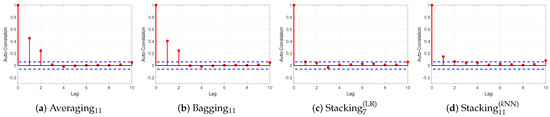
Figure 4. Autocorrelation of residuals for BTC dataset of ensemble models using CNN-LSTM as base learner.

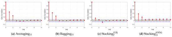
Figure 5. Autocorrelation of residuals for ETH dataset of ensemble models using CNN-LSTM as base learner.

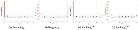
Figure 6. Auto-correlation of residuals for XRP dataset of ensemble models using CNN-LSTM as base learner.

Figure 7, Figure 8 and Figure 9 present the ACF plots of averaging${}_{11}$, bagging${}_{11}$, stacking${}_7^{\left(\mathrm{LR}\right)}$ and stacking${}_{11}^{\left(k\mathrm{NN}\right)}$ ensembles utilizing CNN-BiLSTM as base learner for BTC, ETH and XRP datasets, respectively. Both averaging${}_{11}$ and bagging${}_{11}$ ensemble models violate the assumption of no autocorrelation in the errors, relative to all cryptocurrencies, implying that these models are not properly fitted the time-series. In more detail, the significant spikes at lags 1 and 2 suggest that the residuals are not identically distributed and asymptotically independent, for all datasets. The ACF plot of stacking${}_7^{\left(\mathrm{LR}\right)}$ ensemble for BTC dataset verify that the residuals have no autocorrelation since are within 95% percent confidence interval for all lags. In contrast, for ETH and XRP datasets the spikes at lags 1 and 2 illustrate that there is some autocorrelation of the residuals. Regarding the ACF plots of stacking${}_{11}^{\left(k\mathrm{NN}\right)}$ present that there exists some autocorrelation in the residuals but not particularly large for BTC and XRP datasets; while for ETH dataset, the significant spikes at lags 1 and 2 suggest that the model’s prediction may be inefficient.

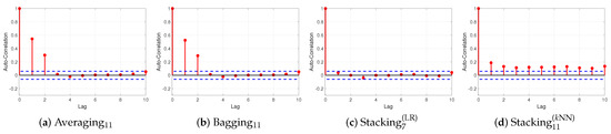
Figure 7. Autocorrelation of residuals for BTC dataset of ensemble models using CNN-BiLSTM as base learner.

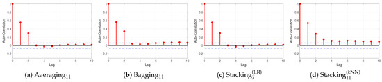
Figure 8. Autocorrelation of residuals for ETH dataset of ensemble models using CNN-BiLSTM as base learner.

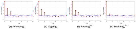
Figure 9. Autocorrelation of residuals for XRP dataset of ensemble models using CNN-BiLSTM as base learner.

6. Discussion

In this section, we perform a discussion regarding the proposed ensemble models, the experimental results and the main finding of this work.

6.1. Discussion of Proposed Methodology

Cryptocurrency prediction is considered a very challenging forecasting problem, since the historical prices follow a random walk process, characterized by large variations in the volatility, although a few hidden patterns may probably exist [48,49]. Therefore, the investigation and the development of a powerful forecasting model for assisting decision making and investment policies is considered essential. In this work, we incorporated advanced deep learning models as base learners into three of the most popular and widely used ensembles methods, namely averaging, bagging and stacking for forecasting cryptocurrency hourly prices.

The motivation behind our approach is to exploit the advantages of ensemble learning and advanced deep learning techniques. More specifically, we aim to exploit the effectiveness of ensemble learning for reducing the bias or variance of error by exploiting multiple learners and the ability of deep learning models to learn the internal representation of the cryptocurrency data. It is worth mentioning that since the component deep learning learners are initialized with different weight states, this leads to the development of deep learning models each of which focuses on different identified patterns. Therefore, the combination of these learners via an ensemble learning strategy may lead to stable and robust prediction model.

In general, deep learning neural networks are powerful prediction models in terms of accuracy, but are usually unstable in sense that variations in their training set or in their weight initialization may significantly affect their performance. Bagging strategy constitutes an effective way of building efficient and stable prediction models, utilizing unstable and diverse base learners [50,51], aiming to reduce variance and avoid overfitting. In other words, bagging stabilizes the unstable deep learning base learners and exploits their prediction accuracy focusing on building an accurate and robust final prediction model. However, the main problem of this approach is that since bagging averages the predictions of all models, redundant and non-informative models may add too much noise on the final prediction result and therefore, possible identified patterns, by some informative and valuable models, may disappear.

On the other hand, stacking ensemble learning utilizes a meta-learner in order to learn the prediction behavior of the base learners, with respect to the final target output. Therefore, it is able to identify the redundant and informative base models and “weight them” in a nonlinear and more intelligent way in order to filter out useless and non-informative base models. As a result, the selection of the meta-learner is of high significance for the effectiveness and efficiency of this ensemble strategy.

6.2. Discussion of Results

All compared ensemble models were evaluated considering both regression and classification problems, namely for the prediction of the cryptocurrency price on the following hour (regression) and also for the prediction if the price will increase or decrease on the following hour (classification). Our experiments revealed that the incorporation of deep learning models into ensemble learning framework improved the prediction accuracy in most cases, compared to a single deep learning model.

Bagging exhibited the best overall score in terms of classification accuracy, closely followed by averaging and stacking${}^{\left(k\mathrm{NN}\right)}$; while stacking${}^{\left(\mathrm{LR}\right)}$ the best regression performance. The confusion matrices revealed that stacking${}^{\left(\mathrm{LR}\right)}$ as base learner was actually biased, since most of the instances were wrongly classified as “Down” while bagging and stacking${}^{\left(k\mathrm{NN}\right)}$ exhibited a balanced prediction distribution between “Down” or “Up” predictions. It is worth noticing that since bagging can be interpreted as a perturbation technique aiming at improving the robustness especially against outliers and highly volatile prices [37]. The numerical experiments demonstrated that averaging ensemble models trained on perturbed training dataset is a means to favor invariance to these perturbations and better capture the directional movements of the presented random walk processes. However, the ACF plots revealed that bagging ensemble models violate the assumption of no autocorrelation in the residuals, which implies that their predictions may be inefficient. In contrast, the ACF plots of stacking${}^{\left(k\mathrm{NN}\right)}$ revealed that the residuals have no or small (inconsiderable) autocorrelation. This is probably due to fact that the use of a meta-learner, which is trained on the errors of the base learners, is able to reduce the autocorrelation in the residuals and provide more reliable forecasts. Finally, it is worth mentioning that the increment of component learners had little or no effect to the regression performance of the ensemble algorithms, in most cases

Summarizing, stacking utilizing advanced deep learning base learner and kNN as meta-learner may considered to be the best forecasting model for the problem of cryptocurrency price prediction and movement, based on our experimental analysis. Nevertheless, further research has to be performed in order to improve the prediction performance of our prediction framework by creating even more innovative and sophisticated algorithmic models. Moreover, additional experiments with respect to the trading-investment profit returns based on such prediction frameworks have to be also performed.

7. Conclusions

In this work, we explored the adoption of ensemble learning strategies with advanced deep learning models for forecasting cryptocurrency price and movement, which constitutes the main contribution of this research. The proposed ensemble models utilize state-of-the-art deep learning models as component learners, which are based on combinations of LSTM, BiLSTM and convolutional layers. An extensive and detailed experimental analysis was performed considering both classification and regression performance evaluation of averaging, bagging, and stacking ensemble strategies. Furthermore, the reliability and the efficiency of the predictions of each ensemble model was studied by examining for autocorrelation of the residuals.

Our numerical experiments revealed that ensemble learning and deep learning may efficiently be adapted to develop strong, stable, and reliable forecasting models. It is worth mentioning that due to the sensitivity of various hyper-parameters of the proposed ensemble models and their high complexity, it is possible that their prediction ability could be further improved by performing additional optimized configuration and mostly feature engineering. Nevertheless, in many real-world applications, the selection of the base learner as well as the specification of their number in an ensemble strategy constitute a significant choice in terms of prediction accuracy, reliability, and computation time/cost. Actually, this fact acts as a limitation of our approach. The incorporation of deep learning models (which are by nature computational inefficient) in an ensemble learning approach, would lead the total training and prediction computation time to be considerably increased. Clearly, such an ensemble model would be inefficient on real-time and dynamic applications tasks with high-frequency inputs/outputs, compared to a single model. However, on low-frequency applications when the objective is the accuracy and reliability, such a model could significantly shine.

Our future work is concentrated on the development of an accurate and reliable decision support system for cryptocurrency forecasting enhanced with new performance metrics based on profits and returns. Additionally, an interesting idea which is worth investigating in the future is that in certain times of global instability, we experience a significant number of outliers in the prices of all cryptocurrencies. To address this problem an intelligent system might be developed based on an anomaly detection framework, utilizing unsupervised algorithms in order to “catch” outliers or other rare signals which could indicate cryptocurrency instability.

References

- Nakamoto, S. Bitcoin: A Peer-to-Peer Electronic Cash System. 2008. Available online: https://git.dhimmel.com/bitcoin-whitepaper/ (accessed on 20 February 2020).
- De Luca, G.; Loperfido, N. A Skew-in-Mean GARCH Model for Financial Returns. In Skew-Elliptical Distributions and Their Applications: A Journey Beyond Normality; Corazza, M., Pizzi, C., Eds.; CRC/Chapman & Hall: Boca Raton, FL, USA, 2004; pp. 205–222. [Google Scholar]
- De Luca, G.; Loperfido, N. Modelling multivariate skewness in financial returns: A SGARCH approach. Eur. J. Financ. 2015, 21, 1113–1131. [Google Scholar] [CrossRef]
- Weigend, A.S. Time Series Prediction: Forecasting the Future and Understanding the Past; Routledge: Abingdon, UK, 2018. [Google Scholar]
- Azoff, E.M. Neural Network Time Series Forecasting of Financial Markets; John Wiley & Sons, Inc.: Hoboken, NJ, USA, 1994. [Google Scholar]
- Oancea, B.; Ciucu, Ş.C. Time series forecasting using neural networks. arXiv 2014, arXiv:1401.1333. [Google Scholar]
- Pintelas, E.; Livieris, I.E.; Stavroyiannis, S.; Kotsilieris, T.; Pintelas, P. Fundamental Research Questions and Proposals on Predicting Cryptocurrency Prices Using DNNs; Technical Report TR20-01; University of Patras: Patras, Greece, 2020; Available online: https://nemertes.lis.upatras.gr/jspui/bitstream/10889/13296/1/TR01-20.pdf (accessed on 20 February 2020).
- Wen, Y.; Yuan, B. Use CNN-LSTM network to analyze secondary market data. In Proceedings of the 2nd International Conference on Innovation in Artificial Intelligence, Shanghai, China, 9–12 March 2018; pp. 54–58. [Google Scholar]
- Liu, S.; Zhang, C.; Ma, J. CNN-LSTM neural network model for quantitative strategy analysis in stock markets. In International Conference on Neural Information Processing; Springer: Berlin/Heidelberg, Germany, 2017; pp. 198–206. [Google Scholar]
- Livieris, I.E.; Pintelas, E.; Pintelas, P. A CNN-LSTM model for gold price time-series forecasting. Neural Comput. Appl. Available online: https://link.springer.com/article/10.1007/s00521-020-04867-x (accessed on 20 February 2020). [CrossRef]
- Pintelas, E.; Livieris, I.E.; Stavroyiannis, S.; Kotsilieris, T.; Pintelas, P. Investigating the problem of cryptocurrency price prediction—A deep learning approach. In Proceedings of the 16th International Conference on Artificial Intelligence Applications and Innovations, Neos Marmaras, Greece, 5–7 June 2020. [Google Scholar]
- Yiying, W.; Yeze, Z. Cryptocurrency Price Analysis with Artificial Intelligence. In Proceedings of the 2019 5th International Conference on Information Management (ICIM), Cambridge, UK, 24–27 March 2019; pp. 97–101. [Google Scholar]
- Nakano, M.; Takahashi, A.; Takahashi, S. Bitcoin technical trading with artificial neural network. Phys. A Stat. Mech. Its Appl. 2018, 510, 587–609. [Google Scholar] [CrossRef]
- McNally, S.; Roche, J.; Caton, S. Predicting the price of Bitcoin using Machine Learning. In Proceedings of the 2018 26th Euromicro International Conference on Parallel, Distributed and Network-based Processing (PDP), Cambridge, UK, 21–23 March 2018; pp. 339–343. [Google Scholar]
- Shintate, T.; Pichl, L. Trend prediction classification for high frequency bitcoin time series with deep learning. J. Risk Financ. Manag. 2019, 12, 17. [Google Scholar] [CrossRef]
- Miura, R.; Pichl, L.; Kaizoji, T. Artificial Neural Networks for Realized Volatility Prediction in Cryptocurrency Time Series. In International Symposium on Neural Networks; Springer: Berlin/Heidelberg, Germany, 2019; pp. 165–172. [Google Scholar]
- Ji, S.; Kim, J.; Im, H. A Comparative Study of Bitcoin Price Prediction Using Deep Learning. Mathematics 2019, 7, 898. [Google Scholar] [CrossRef]
- Kumar, D.; Rath, S. Predicting the Trends of Price for Ethereum Using Deep Learning Techniques. In Artificial Intelligence and Evolutionary Computations in Engineering Systems; Springer: Berlin/Heidelberg, Germany, 2020; pp. 103–114. [Google Scholar]
- Hochreiter, S.; Schmidhuber, J. Long short-term memory. Neural Comput. 1997, 9, 1735–1780. [Google Scholar] [CrossRef] [PubMed]
- Yu, Y.; Si, X.; Hu, C.; Zhang, J. A review of recurrent neural networks: LSTM cells and network architectures. Neural Comput. 2019, 31, 1235–1270. [Google Scholar] [CrossRef] [PubMed]
- Zhang, K.; Chao, W.L.; Sha, F.; Grauman, K. Video summarization with long short-term memory. In European Conference on Computer Vision; Springer: Berlin/Heidelberg, Germany, 2016; pp. 766–782. [Google Scholar]
- Nowak, J.; Taspinar, A.; Scherer, R. LSTM recurrent neural networks for short text and sentiment classification. In International Conference on Artificial Intelligence and Soft Computing; Springer: Berlin/Heidelberg, Germany, 2017; pp. 553–562. [Google Scholar]
- Rahman, L.; Mohammed, N.; Al Azad, A.K. A new LSTM model by introducing biological cell state. In Proceedings of the 2016 3rd International Conference on Electrical Engineering and Information Communication Technology (ICEEICT), Dhaka, Bangladesh, 22–24 September 2016; pp. 1–6. [Google Scholar]
- Schuster, M.; Paliwal, K.K. Bidirectional recurrent neural networks. IEEE Trans. Signal Process. 1997, 45, 2673–2681. [Google Scholar] [CrossRef]
- Graves, A.; Mohamed, A.R.; Hinton, G. Speech recognition with deep recurrent neural networks. In Proceedings of the 2013 IEEE International Conference on Acoustics, Speech and Signal Processing, Vancouver, BC, Canada, 26–31 May 2013; pp. 6645–6649. [Google Scholar]
- Lu, L.; Wang, X.; Carneiro, G.; Yang, L. Deep Learning and Convolutional Neural Networks for Medical Imaging and Clinical Informatics; Springer: Berlin/Heidelberg, Germany, 2019. [Google Scholar]
- Rawat, W.; Wang, Z. Deep convolutional neural networks for image classification: A comprehensive review. Neural Comput. 2017, 29, 2352–2449. [Google Scholar] [CrossRef] [PubMed]
- Michelucci, U. Advanced Applied Deep Learning: Convolutional Neural Networks and Object Detection; Springer: Berlin/Heidelberg, Germany, 2019. [Google Scholar]
- Ioffe, S.; Szegedy, C. Batch normalization: Accelerating deep network training by reducing internal covariate shift. arXiv 2015, arXiv:1502.03167. [Google Scholar]
- Srivastava, N.; Hinton, G.; Krizhevsky, A.; Sutskever, I.; Salakhutdinov, R. Dropout: A simple way to prevent neural networks from overfitting. J. Mach. Learn. Res. 2014, 15, 1929–1958. [Google Scholar]
- Rokach, L. Ensemble Learning: Pattern Classification Using Ensemble Methods; World Scientific Publishing Co Pte Ltd.: Singapore, 2019. [Google Scholar]
- Lior, R. Ensemble Learning: Pattern Classification Using Ensemble Methods; World Scientific: Singapore, 2019; Volume 85. [Google Scholar]
- Zhou, Z.H. Ensemble Methods: Foundations and Algorithms; Chapman & Hall/CRC: Boca Raton, FL, USA, 2012. [Google Scholar]
- Bian, S.; Wang, W. On diversity and accuracy of homogeneous and heterogeneous ensembles. Int. J. Hybrid Intell. Syst. 2007, 4, 103–128. [Google Scholar] [CrossRef]
- Polikar, R. Ensemble learning. In Ensemble Machine Learning; Springer: Berlin/Heidelberg, Germany, 2012; pp. 1–34. [Google Scholar]
- Christiansen, B. Ensemble averaging and the curse of dimensionality. J. Clim. 2018, 31, 1587–1596. [Google Scholar] [CrossRef]
- Grandvalet, Y. Bagging equalizes influence. Mach. Learn. 2004, 55, 251–270. [Google Scholar] [CrossRef]
- Livieris, I.E.; Iliadis, L.; Pintelas, P. On ensemble techniques of weight-constrained neural networks. Evol. Syst. 2020, 1–3. [Google Scholar] [CrossRef]
- Wolpert, D.H. Stacked generalization. Neural Netw. 1992, 5, 241–259. [Google Scholar] [CrossRef]
- Gulli, A.; Pal, S. Deep Learning with Keras; Packt Publishing Ltd.: Birmingham, UK, 2017. [Google Scholar]
- Kingma, D.P.; Ba, J. Adam: A method for stochastic optimization. In Proceedings of the 2015 International Conference on Learning Representations, San Diego, CA, USA, 7–9 May 2015. [Google Scholar]
- Wu, X.; Kumar, V. The Top Ten Algorithms in Data Mining; CRC Press: Boca Raton, FL, USA, 2009. [Google Scholar]
- Deng, N.; Tian, Y.; Zhang, C. Support Vector Machines: Optimization Based Theory, Algorithms, and Extensions; Chapman and Hall/CRC: Boca Raton, FL, USA, 2012. [Google Scholar]
- Kutner, M.H.; Nachtsheim, C.J.; Neter, J.; Li, W. Applied Linear Statistical Models; McGraw-Hill Irwin: New York, NY, USA, 2005; Volume 5. [Google Scholar]
- Aha, D.W. Lazy learning; Springer Science & Business Media: Berlin/Heidelberg, Germany, 2013. [Google Scholar]
- Breiman, L.; Friedman, J.; Olshen, R. Classification and Regression Trees; Routledge: Abingdon, UK, 2017. [Google Scholar]
- Brockwell, P.J.; Davis, R.A. Introduction to Time Series and Forecasting; Springer: Berlin/Heidelberg, Germany, 2016. [Google Scholar]
- Stavroyiannis, S. Can Bitcoin diversify significantly a portfolio? Int. J. Econ. Bus. Res. 2019, 18, 399–411. [Google Scholar] [CrossRef]
- Stavroyiannis, S. Value-at-Risk and Expected Shortfall for the major digital currencies. arXiv 2017, arXiv:1708.09343. [Google Scholar] [CrossRef][Green Version]
- Elisseeff, A.; Evgeniou, T.; Pontil, M. Stability of randomized learning algorithms. J. Mach. Learn. Res. 2005, 6, 55–79. [Google Scholar]
- Kotsiantis, S.B. Bagging and boosting variants for handling classifications problems: A survey. Knowl. Eng. Rev. 2014, 29, 78–100. [Google Scholar] [CrossRef]
© 2020 by the authors. Licensee MDPI, Basel, Switzerland. This article is an open access article distributed under the terms and conditions of the Creative Commons Attribution (CC BY) license (http://creativecommons.org/licenses/by/4.0/).