Numerical Simulation of Non-Linear Models of Reaction—Diffusion for a DGT Sensor

Abstract

In this work, we present a novel strategy for the numerical solution of a coupled system of partial differential equations that describe reaction–diffusion processes of a mixture of metals and ligands that can be absorbed by a sensor or a microorganism, in an aqueous medium. The novelty introduced in this work consisted of an adequate database management in conjunction with a direct iterative schema, which allowed the construction of simple, fast and efficient algorithms. Except in really adverse conditions, the calculation is converging and satisfactory solutions were reached. Computing times showed to be better than those obtained with some commercial programs. Although we concentrate on the solution for a particular system (Diffusive Gradients in Thin Films [DGT] sensors), the proposed algorithm does not require major modifications to consider new theoretical or experimental configurations. Since the quality of numerical simulations of reaction–diffusion problems often faces some drawbacks as the values of reaction rate constants increase, some additional effort has been invested in obtaining proper solutions in those cases.

1. Introduction

The high risk of contamination due to the presence of heavy metals in aqueous systems requires the development of reliable analytical techniques, capable of measuring the metal flux that reaches microorganisms, algae, plants or other live organisms present in the media [1].

Generally, in aquatic ecosystems, the metal flux toward an interface where it is consumed (for instance, by an organism or an analytical sensor), is the result of diffusion and kinetics of interconversion between metal and the various species present in the system (see scheme outlined in Figure 1).

A quantitative assessment of the metal flux that reaches a consuming interface requires the rigorous solution of the resulting system of transport and reaction equations, taking into account the geometry and the temporal and spatial scales. The mathematical models that describe these reaction–diffusion processes consist of systems of partial differential equations (PDE) with polynomial reaction terms [2].

For instance, if the ML species schematized in Figure 1 reacts as follows:

$$\mathrm{M}+\mathrm{L}\underset{k_{\mathrm{d},1}}{\overset{k_{\mathrm{a},1}}{\rightleftarrows }}\mathrm{ML}$$

(1)

and

$$\mathrm{ML}+\mathrm{L}\underset{k_{\mathrm{d},2}}{\overset{k_{\mathrm{a},2}}{\rightleftarrows }}{\mathrm{ML}}_2,$$

(2)

the change of ML concentration (c_ML) with time will be given by [3]

$$\frac{\partial c_{\mathrm{ML}}}{\partial t}=D_{\mathrm{ML}}\frac{{\partial }^2{c}_{\mathrm{ML}}}{\partial x^2}-k_{\mathrm{a},1}{c}_{\mathrm{ML}}{c}_{\mathrm{M}}+k_{\mathrm{d},1}{c}_{\mathrm{ML}}-k_{\mathrm{a},2}{c}_{\mathrm{ML}}{c}_{\mathrm{L}}+k_{\mathrm{d},2}{c}_{{\mathrm{ML}}_2},$$

(3)

where $c_i$ is the concentration of specie i, t stands for the time, x represents the spatial dimension, D_ML is the diffusion coefficient of the ML species, and $k_{\mathrm{a},i}$, $k_{\mathrm{d},i}$ ($i=1,2$) represent the association and the dissociation rate constants given in reactions (1) and (2).

In general, for any species i in the media ($i=$ M, L, ML, ML${}_2$, …), the variation of the concentration with time will depend on the diffusive term plus the reaction terms, as follows:

$$\frac{\partial c_i}{\partial t}=D_i\frac{{\partial }^2{c}_i}{\partial x^2}+«\mathrm{reaction}\mathrm{terms}».$$

(4)

Thus, the system will contain as many equations as species, coupled by the reaction terms. However, in most practical cases, the resulting system of PDE cannot be analytically solved. In these cases, numerical approximations will be the only way to reach solutions for these systems.

The most common form of solving these systems consists of, as a first step, the discretization of equations, which transforms the differential system in an algebraic system different for each increase of time. Next, when the resulting system is non-linear, it could be solved by Newton-type techniques [4].

In this second step, two difficulties can be mentioned. The lower one is the lack of robustness of the method, which requires the introduction of Armijo or norm minimization strategies [5], to improve the convergence of the iterative process. However, the greatest obstacle appears as a consequence of the dimension of the linear system (n). In these problems, the number of unknown variables, n, is equal to the product of the number of species by the number of nodes in the spatial discretization. Considering that n may be large and that resolution time of a linear equations system is of the order of $n^3/3$ s [5], the computational cost can be unaffordable in a general-purpose computer.

In this work, a set of algorithms that allow simulating systems with a large number of chemical species, and with a computational cost that supports the simulation of processes of some complexity in a reasonably short time, are presented. For this, Section 2 introduces the theoretical framework and the mathematical model. Section 3 discusses the iterative resolution of the system. Section 4 shows the results and analysis. The Appendix A contains the general resolution algorithm.

2. The Model

The proposed algorithm was developed to solve the reaction-diffusion equations that model the operation of a Diffusive Gradients in Thin Films (DGT) sensor [6], submerged in an aqueous solution containing different metal species. Nevertheless, the algorithm does not require major modifications to consider new theoretical or experimental configurations.

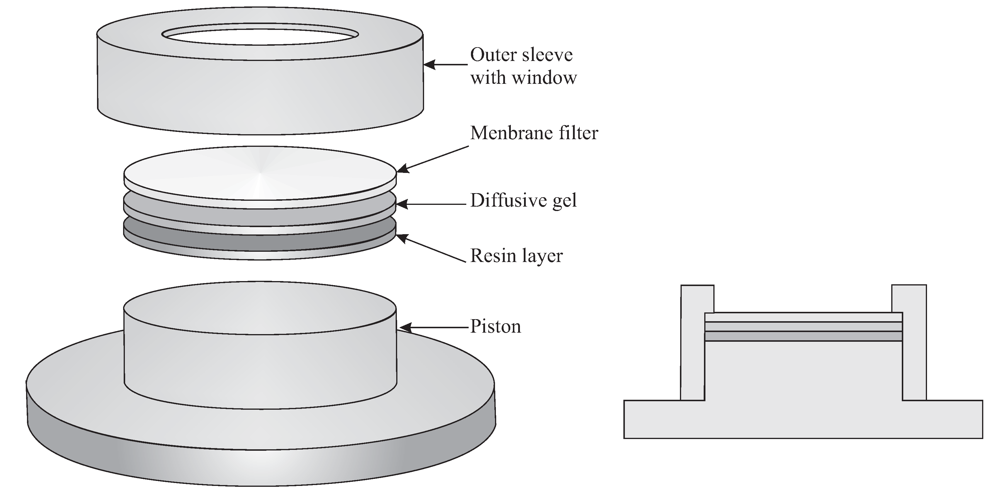
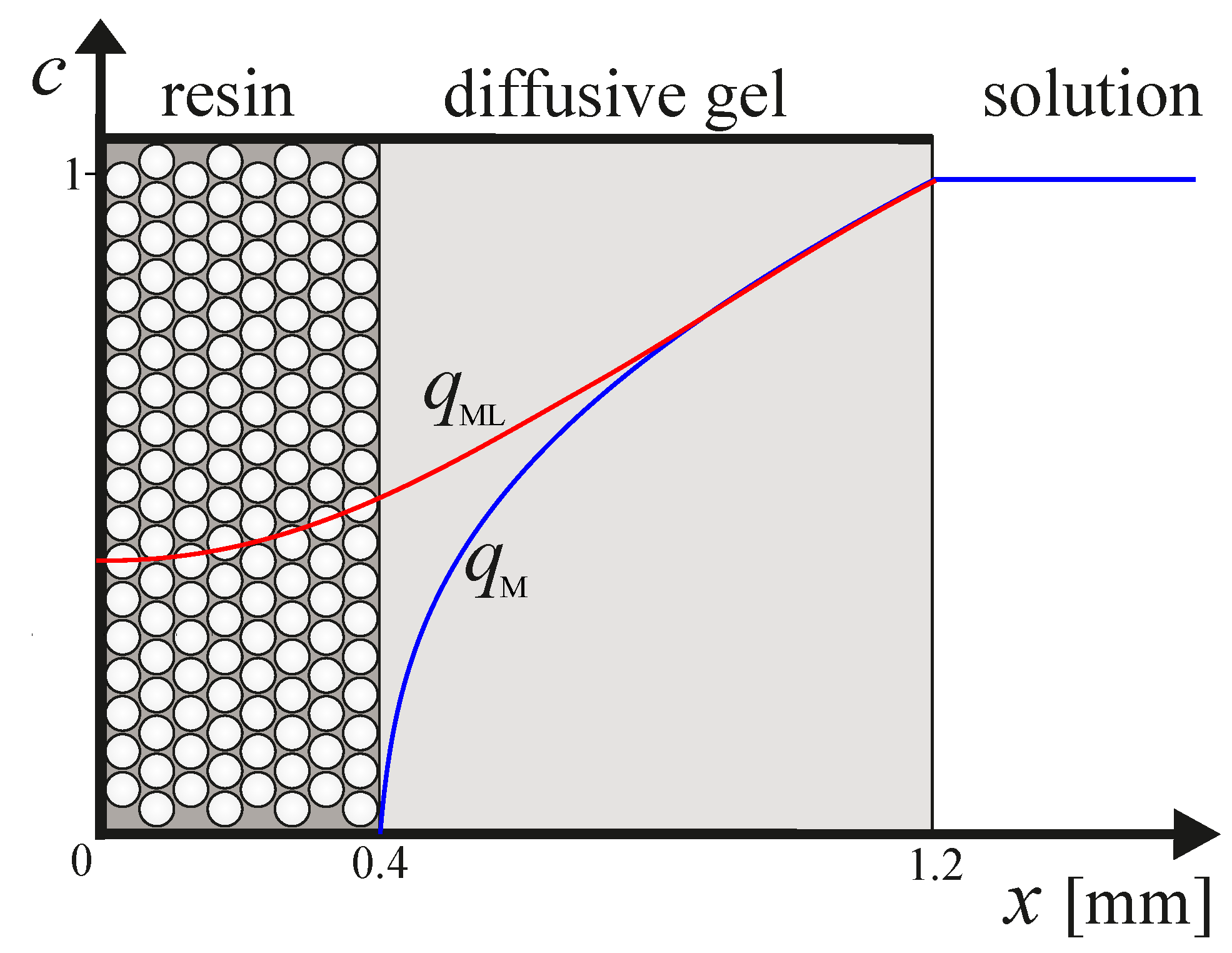
2.1. Diffusive Gradients in Thin Films (DGT)

The analytical technique known as DGT consists of simple devices developed for the in-situ measurement of bioavailability of heavy metals in soils and aquatic environments [6,7].

The DGT sensors are made up of three layers (see Figure 2): a hydrogel layer impregnated with a complexing material (resin layer), a hydrogel used as a diffusion layer, and a membrane filter. These three layers are placed in a plastic holder device [7].

DGT sensors were designed to emulate the metal absorption process in aqueous media. When a DGT is deployed in a sampling solution, where all species are in equilibrium, the metal species diffuse through the diffusive gel (where they might associate or dissociate), toward the resin layer where they accumulate as metal resin complexes.

As long as the resin does not get saturated, a concentration gradient is maintained in the diffusion layer. Very soon, (quasi) steady-state conditions are reached, so the initial transient can be neglected to obtain easy approximate analytical expressions. Fick’s first law of diffusion describes the flux ($J_i$) for each species i,

$$J_i=D_i\frac{\mathrm{d}{c}_i}{\mathrm{d}x},$$

(5)

where $D_i$ is the diffusion coefficient, $c_i$ is the concentration and d$c_i$/dx is the gradient of spatial concentration of the i species.

After the DGT has been exposed to the solution, it must be opened and the analytes eluted from the resin to be quantified.

When only metal is present in the solution, the accumulated mass in DGT is related to the solution concentration through a simple equation that neglects the effects of dynamic speciation [6]:

$$n=D\frac{c_{\mathrm{M}}^{\ast }}{g}At,$$

(6)

where n stands for the accumulated moles, D represents an average diffusion coefficient, $c_{\mathrm{M}}^{\ast }$ is the metal concentration at the solution, A is the DGT area, t is the deployment time, and g is the diffusion layer thickness.

In the presence of metal complexes, $c_{\mathrm{M}}^{\ast }$ is replaced with $c_{\mathrm{DGT}}^{\ast }$, which indicates the effective or apparent metal concentration leading to this accumulation. $c_{\mathrm{DGT}}^{\ast }$ is usually called the labile metal concentration of the solution.

The rigorous interpretation of $c_{\mathrm{DGT}}^{\ast }$ in terms of the real species in solutions requires taking into account all reaction–diffusion processes involved in the system, which can only be achieved via numerical simulation.

2.2. Mathematical Model

Consider the complexation of different metals and ligands in solution, that react according to the elementary schema represented in the Equation (7):

$$\mathrm{A}+\mathrm{B}\underset{k_{\mathrm{d}}}{\overset{k_{\mathrm{a}}}{\rightleftarrows }}\mathrm{AB},$$

(7)

where A and B can represent a metal, a ligand, or any combination of them, and $k_{\mathrm{a}}$ and $k_{\mathrm{d}}$ represent the kinetic constants of association and dissociation, respectively. The equilibrium conditions for this reaction are expressed in the form

$$K=\frac{k_{\mathrm{a}}}{k_{\mathrm{d}}}=\frac{c_{\mathrm{AB}}^{\ast }}{c_{\mathrm{A}}^{\ast }{c}_{\mathrm{B}}^{\ast }},$$

(8)

where K is the equilibrium constant, and $c_i^{\ast }$ indicates the concentration of species i in the solution (bulk concentration).

When a DGT sensor is deployed in solution, the species diffuse to the resin (located between $0<x<r$), through the gel layer between $r<x<r+g$ (see Figure 3).

Inside the DGT, the concentration $c(x,t)$ of each species is modified by diffusion, reaction with other species present in the solution, and by the possible reaction with the resin.

Before presenting the mathematical formulation, we will make some assumptions.

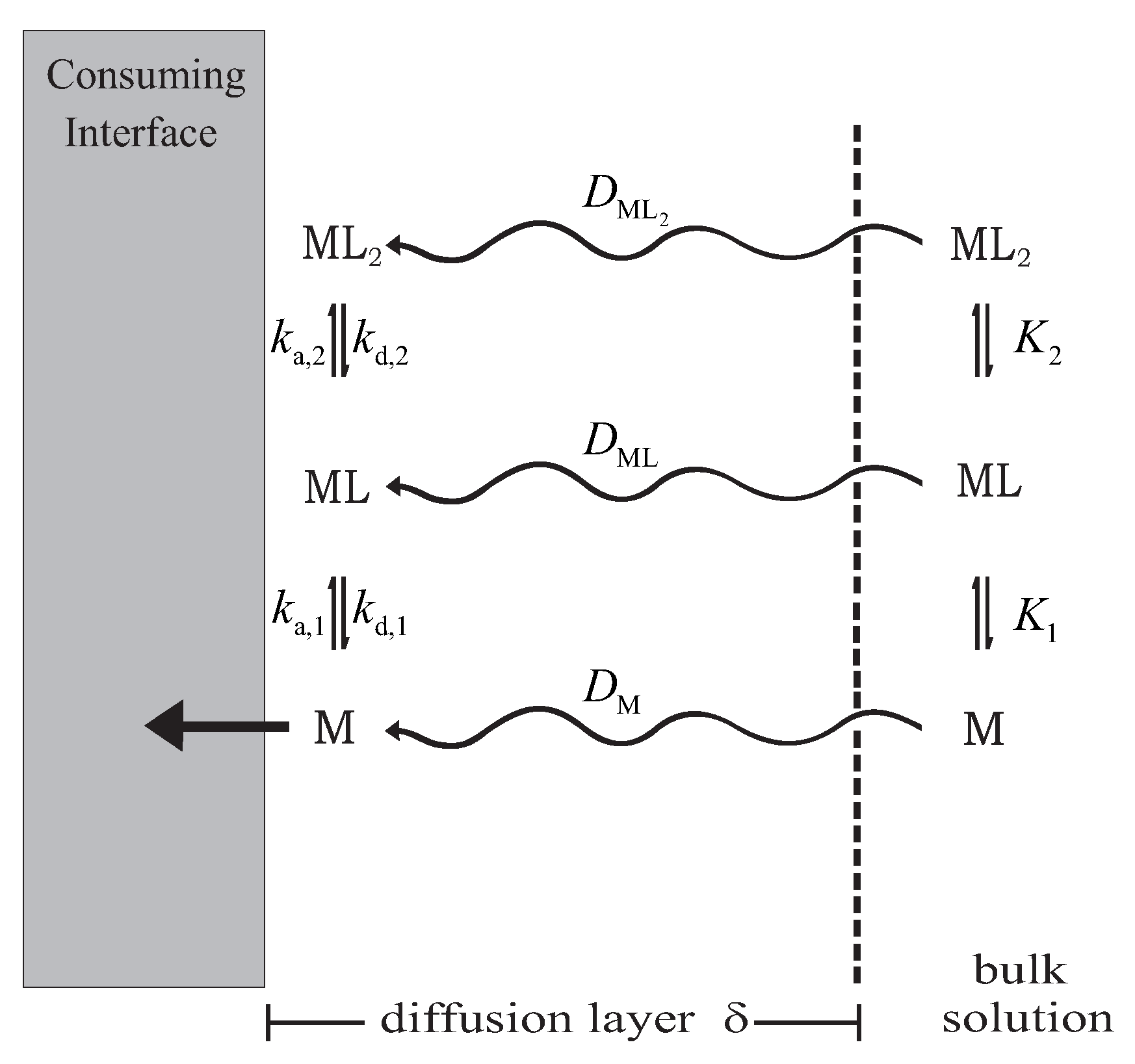
• Since the resin discs are made of complexing material embedded in the same type of gel that composes the diffusive layer, it is reasonable to consider that species that diffuse through the gel can penetrate the resin [8].
• Species that diffuse through the gel can bind the resin after. They do it by the described schema in Equation (9):

  $$\mathrm{A}+\mathrm{R}\underset{k_{\mathrm{d},\mathrm{R}}}{\overset{k_{\mathrm{a},\mathrm{R}}}{\rightleftarrows }}\mathrm{AR},$$

  (9)

  where R denotes the free-sites in the interior of the resin, and $k_{\mathrm{a},\mathrm{R}}$, $k_{\mathrm{d},\mathrm{R}}$ and ${\mathrm{K}}_{\mathrm{R}}=k_{\mathrm{a},\mathrm{R}}/k_{\mathrm{d},\mathrm{R}}$ represent the corresponding kinetic and stability constants.
• When the material used for the resin is Chelex, the grains of resin are located mainly in the layer adjacent to the diffusion gel [9]. In a first approach, we consider that binding sites in the resin are uniformly distributed.
• Because diffusion coefficients in the gel, the filter and diffusive boundary layer (DBL) are similar [10], the diffusive layer width g in Figure 3 includes the size of all these layers.
• Migration forces or any electrostatic effects due to the charge of resin are not considered, i.e., the background salt is enough to screen these interactions.

Under these conditions, diffusion is the most relevant transport mechanism in the system and, therefore, the transport equations for each species i can be written as

$$\begin{array}{c}\hfill \frac{\partial c_i}{\partial t}=D_i^{\mathrm{R}}\frac{{\partial }^2{c}_i}{\partial x^2}+«\mathrm{reaction}\mathrm{terms}»\mathrm{for}0<x<r;\mathrm{and}\\ \hfill \frac{\partial c_i}{\partial t}=D_i\frac{{\partial }^2{c}_i}{\partial x^2}+«\mathrm{reaction}\mathrm{terms}»\mathrm{for}r<x<r+g,\end{array}$$

(10)

where $D_i^{\mathrm{R}}$ and $D_i$ are diffusion coefficients of the species i in the resin and gel, respectively, and the so-called «terms of reaction» refer to the kinetic terms corresponding to the reaction of the specie i with other substances of the solution.

Technically, the expressions shown in Equation (10) are second-order parabolic partial differential equations that can be analytically solved only under very specific conditions.

In general, in the cases of practical interest, these equations do not have analytical solutions. Thus, numerical solutions may be the best way to get the concentration values for each point of space in every instant of time.

As described in the introduction, the most widely used approach to numerically solve these systems consists of discretizing the equations and, subsequently, iteratively solve the resulting system of algebraic equations. The following sections describe a novel strategy to numerically solve the systems of equations of the form (10).

2.3. The Problem

Let us consider a set of elementary reactions, in a number equal to $numreac$, of the form

$$\begin{array}{c}\hfill \begin{array}{cc}{\mathrm{X}}_{{\mathrm{L}}_{11}}+{\mathrm{X}}_{{\mathrm{L}}_{12}}\underset{k_{\mathrm{d},1}}{\overset{k_{\mathrm{a},1}}{\rightleftarrows }}{\mathrm{X}}_{{\mathrm{L}}_{13}}& \mathrm{Reaction}1,\\ {\mathrm{X}}_{{\mathrm{L}}_{21}}+{\mathrm{X}}_{{\mathrm{L}}_{22}}\underset{k_{\mathrm{d},2}}{\overset{k_{\mathrm{a},2}}{\rightleftarrows }}{\mathrm{X}}_{{\mathrm{L}}_{23}}& \mathrm{Reaction}2,\\ ⋮& ⋮\\ {\mathrm{X}}_{{\mathrm{L}}_{j1}}+{\mathrm{X}}_{{\mathrm{L}}_{j2}}\underset{k_{\mathrm{d},j}}{\overset{k_{\mathrm{a},j}}{\rightleftarrows }}{\mathrm{X}}_{{\mathrm{L}}_{j3}}& \mathrm{Reaction}j,\\ ⋮& ⋮\end{array}\end{array}$$

(11)

where $k_{\mathrm{a},j}$, $k_{\mathrm{d},j}$ and $K_j=k_{\mathrm{a},j}/k_{\mathrm{d},j}$, for $j=1,2,\dots ,numreac$, represent the kinetic and stability constants, respectively. It is worth mentioning that in the set of reactions (11) some species could be repeated, e.g., ${\mathrm{X}}_{{\mathrm{L}}_{11}}$ might be equal to ${\mathrm{X}}_{{\mathrm{L}}_{21}}$

The system is encoded according to the indexing used in Equation (11), without any restrictions on the number of metals or ligands. As it has already been said, the only restriction is that all chemical reactions should be written in the form $\mathrm{A}+\mathrm{B}\rightleftharpoons \mathrm{C}$.

Given that starting data are the total concentrations of the pure substances (i.e., those that are not the result of a reaction), it is first necessary to solve the equilibrium problem, that is to say, it is needed to find the concentration value in solution (or bulk concentration) for each of the species in the system.

To do this we build $mreac$ and $kreac$, arrays that allow introducing the information related to the chemical reactions that must be considered in $x=r+g$. The first of these arrays, $mreac$, is the index array that contains three columns and a number of rows equal to the number of $numreac$ reactions,

$$mreac=\left(\begin{array}{ccc}{L}_{11}& L_{12}& L_{13}\\ L_{21}& L_{22}& L_{23}\\ ⋮& ⋮& ⋮\\ L_{j1}& L_{j2}& L_{j3}\\ ⋮& ⋮& ⋮\end{array}\right).$$

(12)

The $mreac$ array is constructed in such a way that, if in the j-th reaction the substance 5 is combined with the 7 to produce 8, the indices of the row j will be $578$; that is, the first two columns contain the components and the third indicates the formed compound.

The $kreac$ matrix contains the same number of rows as the $mreac$ matrix, but only two columns. The first column indicates the value of the association constant ($k_{\mathrm{a},j}$), and the second one the value of the dissociation constant ($k_{\mathrm{d},j}$) of each j reaction, with $j=1,2,\dots ,numreac$,

$$kreac=\left(\begin{array}{cc}{k}_{\mathrm{a}1}& k_{\mathrm{d}1}\\ k_{\mathrm{a}2}& k_{\mathrm{d}2}\\ ⋮& ⋮\\ k_{\mathrm{a}j}& k_{\mathrm{d}j}\\ ⋮& ⋮\end{array}\right).$$

(13)

The strategy to solve the problem is to express the non-pure of species (i.e., species that are listed in the third column of $mreac$, because they are the result of a reaction), as a combination of the total concentrations of the pure substances, which are known for the system. The result is a system of nonlinear equations, which is solved using a variation of the Newton–Raphson method.

Once the equilibrium problem is solved, that is to say, once the bulk concentration values are obtained for each species at $t=0$ and $x=r+g$, it is necessary to pose the problem of transport for an arbitrary number of chemical species.

Let $numeq$ be the number of species of the problem, which, of course, coincides with the number of equations. In the first place two vectors of coefficients are considered, one for the region $(0;r)$, hereinafter referred to as: ${\overrightarrow{D}}^{\mathrm{R}}=(D_1^{\mathrm{R}},D_2^{\mathrm{R}},\dots ,D_{numeq}^{\mathrm{R}})$, which contains the diffusion coefficient for each species inside the resin phase, and the other denoted by $\overrightarrow{D}=(D_1,D_2,\dots ,D_{numeq})$, which corresponds to diffusion coefficients inside the gel ($r<x<r+g$). Diffusion coefficients of the resin and its complexes are zero since they are considered to be fixed in the gel matrix of the resin disc.

The $mreac$ and $kreac$ matrices, that were used for solving the equilibrium problem, must be extended incorporating the reactions corresponding to the resin and its complexes.

These two new matrices contain the information to express the general problem. For each species i, where $i=1,\dots ,numeq$, the corresponding reaction–diffusion equation will be as:

$$\frac{\partial c_i}{\partial t}=\left\{\begin{array}{c}{D}_i^{\mathrm{R}}\\ D_i\end{array}\right\}\frac{{\partial }^2{c}_i}{\partial x^2}+\sum _{j=1}^{numreac}(A_{i,j}{c}_{mreac(j,1)}{c}_{mreac(j,2)}+B_{i,j}{c}_{mreac(j,3)}),$$

(14)

where $D_i^{\mathrm{R}}$ and $D_i$ act as a diffusion coefficients in $(0,r)$ and $(r,r+g)$, respectively.

In Equation (14), for a given value of index i (which runs across chemical species), the coefficients $A_{i,j}$ and $B_{i,j}$ can be calculated using the following algorithm: if in the reaction j does not participate the species i, $A_{i,j}=B_{i,j}=0$. Otherwise, the absolute value of $A_{i,j}$ is equal to $k_{\mathrm{a},j}$ and the absolute value of $B_{i,j}$ is equal to $k_{\mathrm{d},j}$. Finally, it must be taken into account that the coefficient ($A_{i,j}$ or $B_{i,j}$) of the term that contains the substance i-th must be negative.

2.4. Initial and Boundary Conditions

When the DGT is deployed in the solution, at time $t=0$ the concentration of each of the species i inside the spatial domain $(0,r+g)$ is zero, that is $c_i(x,0)=0$, except for the free places inside the resin, whose initial concentration is $c_{\mathrm{R}}(x,0)=c_{\mathrm{TR}}$ (the total concentration of resin sites).

Resin sites are considered immobile, but for species with $D_i\ne 0$, it must be considered one boundary condition at $x=r+g$, i.e., at the interface between the diffusive gel and the solution:

$$c_i(r+g,t)=c_i^{\ast },$$

where $c_i^{\ast }$ stands for the bulk concentration of species i.

At the DGT bottom, i.e., at $x=0$, there should be no flow of any species,

$${\left.\frac{\partial c_i}{\partial x}\right|}_{x=0}=0.$$

Finally, at the resin–gel interface ($x=r$), there must be continuity in the concentration profiles and flows of each species,

$$c_i(r^{-},t)=c_i(r^{+},t);D_i^{\mathrm{R}}{\left.\frac{\partial c_i}{\partial x}\right|}_{x=r^{-}}=D_i{\left.\frac{\partial c_i}{\partial x}\right|}_{x=r^{+}}.$$

2.5. Dimensionless Formulation

To adapt scales to the order of magnitude of data, the variable changes that lead to the nondimensional problem, are described.

• For all species in solution, that is, for all the species that have a bulk solution concentration, obtained from the solution of the equilibrium problem, we define standard concentrations,

  $$q_i=\frac{c_i}{c_i^{\ast }}.$$
• For the rest, that is to say, the resin and its complexes,

  $$q_j=\frac{c_j}{c_{\mathrm{TR}}}.$$
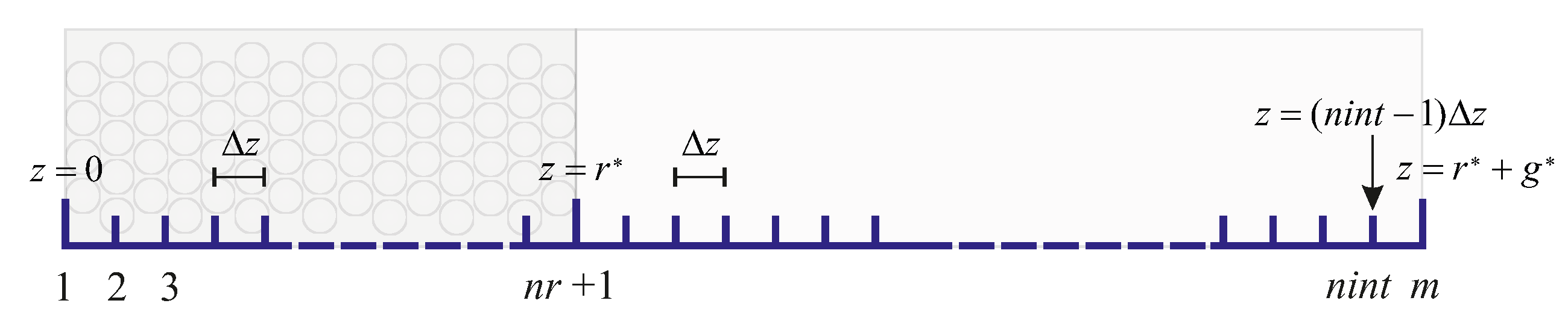
• For the spatial coordinate, instead of nondimensionalisation, a change of scale is used,

  $$z=\frac{x}{\sqrt{D_{\max }}},$$

  where $D_{\max }$ is the highest diffusion coefficient. It makes it necessary to define $r^{\ast }=r/\sqrt{D_{\max }}$; $g^{\ast }=g/\sqrt{D_{\max }}$; $d_i=D_i/D_{\max }$; and $d_i^{\mathrm{R}}=D_i^{\mathrm{R}}/D_{\max }$.
• Given that the aim is to simulate experiments involving different time scales, the time axis is not changed.

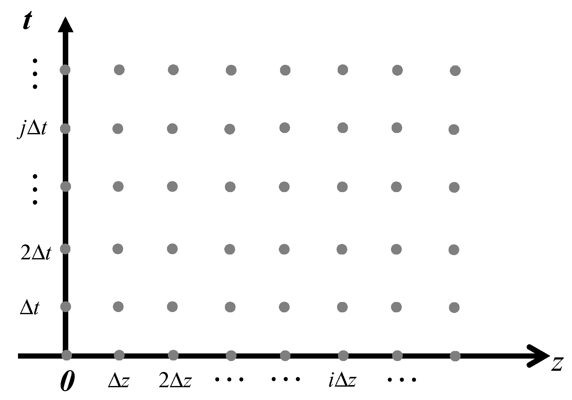
With these new variables, the reaction–diffusion equations described in Equation (14) are rewritten as follows:

$$\frac{\partial q_i}{\partial t}=\left\{\begin{array}{c}{d}_i^{\mathrm{R}}\\ d_i\end{array}\right\}\frac{{\partial }^2{q}_i}{\partial z^2}+\sum _{j=1}^{numreac}({\widehat{A}}_{i,j}{q}_{mreac(j,1)}{q}_{mreac(j,2)}+{\widehat{B}}_{i,j}{q}_{mreac(j,3)}),$$

(15)

where $d_i^{\mathrm{R}}$ acts as a diffusion coefficient in$(0,r^{\ast })$ and $d_i$ in $(r^{\ast },r^{\ast }+g^{\ast })$, and where the new coefficients ${\widehat{A}}_{i,j}$ and ${\widehat{B}}_{i,j}$ are calculated as

$${\widehat{A}}_{i,j}=A_{i,j}\frac{c_{mreac(j,1)}^{\ast }{c}_{mreac(j,2)}^{\ast }}{c_i^{\ast }};{\widehat{B}}_{i,j}=B_{i,j}\frac{c_{mreac(j,3)}^{\ast }}{c_i^{\ast }}.$$

(16)

For the concentrations of the resin and its complexes, $c_i^{\ast }$ must be replaced by $c_{\mathrm{TR}}$.

The initial and boundary conditions for all substances that do not contain resin, that is to say, for all those whose diffusion coefficient is different from zero, are now

$$q_i(z,0)=0;q_i(r^{\ast }+g^{\ast },t)=1,$$

(17)

and

$$\begin{array}{cc}\hfill {\left.\frac{\partial q_i}{\partial z}\right|}_{z=0}& =0,\hfill \\ \hfill q_i(r^{\ast -},t)& =q_i(r^{\ast +},t),\hfill \\ \hfill {\left.\frac{\partial q_i}{\partial z}\right|}_{z=r^{\ast -}}& =\frac{d_i}{d_i^R}{\left.\frac{\partial q_i}{\partial z}\right|}_{z=r^{\ast +}}.\hfill \end{array}$$

(18)

The remaining substances only need an initial condition: for the resin

$$q_{\mathrm{R}}(z,0)=\left\{\begin{array}{cc}1\hfill & \mathrm{si}0<z<r^{\ast }\hfill \\ 0\hfill & \mathrm{si}{r}^{\ast }<z<r^{\ast }+g^{\ast }\hfill \end{array}\right.$$

For complexes of the resin $q_i(x,0)=0$ in $(0,r^{\ast }+g^{\ast })$.

2.6. Discretization

The spatial discretization of a PDE model can be performed using different techniques. The most frequently used are those of finite differences, finite element (with all its variants) or finite volumes [4,11]. Each of these techniques has its advantages and disadvantages. For instance, discretizing by the finite difference method leads to simple computer programming, as long as fixed spatial steps are used. However, this latter could imply the use of a large number of points and, therefore, longer calculation times.

On the other hand, the finite element method allows working with arbitrary point distributions, using smaller spatial steps in regions where it is assumed that function could rapidly changes, so error in the iteration could be large, and larger widths where it is known that the error will be smaller [12]. Although this flexibility results in a computational cost lower than in the case of the finite differences, it involves an algorithmic and programming effort that can be significantly high.

In this work, the finite differences method was used, taking fixed spatial steps of length $\Delta z$, and temporal intervals equal to $\Delta t$ (see Figure 4).

Let $F(z,t)$ be a function that can contain spatial derivatives (of different orders) of the function $f(z,t)$. If

$$\frac{\partial f(z,t)}{\partial t}=F(z,t),$$

(19)

Equation (19) can be discretized as a linear combination of the form

$$\frac{f(z_i,t+\Delta t)-f(z_i,t)}{\Delta t}\simeq \lambda F(z_i,t+\Delta t)+(1-\lambda )F(z_i,t),$$

(20)

where, $0\le \lambda \le 1$.

In general, for the PDE of parabolic type, the backward Euler method for discretization (i.e., taking $\lambda =1$ in Equation (20)), allows choosing arbitrary increases in z and t, without risking its stability or introducing spurious oscillations in the iterative process [4].

Next, for every substance i, the differential Equation (15) will by discretized using the backward Euler scheme to obtain a system of algebraic equations.

For species with diffusion coefficient different from zero, the Equation (15) is transformed into

$$\begin{array}{cc}\hfill \frac{q_i(z,t+\Delta t)-q_i(z,t)}{\Delta t}& =\left\{\begin{array}{c}{d}_i^{\mathrm{R}}\\ d_i\end{array}\right\}\frac{q_i(z+\Delta z,t+\Delta t)-2q_i(z,t+\Delta t)+q_i(z-\Delta z,t+\Delta t)}{\Delta z^2}\hfill \\ \hfill & +\sum _{j=1}^{numreac}{\widehat{A}}_{i,j}{q}_{mreac(j,1)}(z,t+\Delta t)q_{mreac(j,2)}(z,t+\Delta t)+{\widehat{B}}_{i,j}{q}_{mreac(j,3)}(z,t+\Delta t).\hfill \end{array}$$

(21)

In this case, the described boundary conditions in Equations (17) and (18) will be

$$\begin{array}{cc}\hfill q_i(\Delta z,t+\Delta t)-q_i(0,t+\Delta t)& =0,\hfill \\ \hfill q_i(r^{\ast }+g^{\ast },t+\Delta t)& =1,\hfill \end{array}$$

(22)

and

$$q_i(r,t+\Delta t)-q_i(r-\Delta z,t+\Delta t)=\frac{d_i}{d_i^R}\left[q_i(r+\Delta z,t+\Delta t)-q_i(r,t+\Delta t)\right].$$

(23)

There is no need for any expression for the solution continuity at $z=r^{\ast }$. Simply, from now on, it will be considered for such a position, that each substance has a unique concentration value (a simple way to state that it is continuous, due to the absence of electrostatic effects).

Due to the fact that the resin and its components are considered motionless, the differential equations for these substances do not contain spatial derivatives. In this way, the equations described in (15) for species with zero coefficient diffusion are re-written as follows:

$$\begin{array}{cc}\hfill \frac{q_i(z,t+\Delta t)-q_i(z,t)}{\Delta t}& =\sum _{j=1}^{numreac}{\widehat{A}}_{i,j}^{\mathrm{R}}{q}_{mreac(j,1)}(z,t+\Delta t)q_{mreac(j,2)}(z,t+\Delta t)\hfill \\ \hfill & +{\widehat{B}}_{i,j}^{\mathrm{R}}{q}_{mreac(j,3)}(z,t+\Delta t),\hfill \end{array}$$

(24)

for $(0,r^{\ast })$, and

$$q_i(z,t+\Delta t)=0,\forall z\in (r^{\ast },r^{\ast }+g^{\ast }).$$

(25)

3. Iterative Resolution of the Resulting System of Equations

In Equations (21) and (24), the terms derived from reactions couple the resulting algebraic equation system, by involving second-order terms as products of concentrations from different species. As mentioned in the introduction, these types of non-linear systems are generally solved by using iterative-type Newton techniques. The novelty introduced in this work consisted in convenient database management operated in conjunction with a direct iterative schema, which allowed us the construction of simple, fast and efficient algorithms for solving reaction–diffusion problems.

The basic idea of these algorithms consists on the assumption that the solution for all species is known at time t; then, the solution at time $t+\Delta t$ is obtained according to the following scheme:

1.

Initialize all concentrations at $t+\Delta t$ with the solution at time t.

2.

for$i=1,numeq$

To solve discrete i-th equation (for the species i-th) considering all other j-th species ($i\ne j$) constant in this stage and whose value at $t+\Delta t$ being the corresponding to its most recent calculation.

endfor

3.

Repeat step 2 until the difference between concentrations in two consecutive iterations be less than a small fixed value.

The described iterative structure has the advantage that resolution, for each substance i with diffusion coefficient different from zero, is reduced to a tridiagonal system in which the diagonal is strongly dominant, due to the negative sign of the terms that contain $c_i$. Even better, for the resin and its complexes, species for which the diffusion coefficient is zero, the system is diagonal.

All this results in a great increase on calculating speed, since it is better to solve a dozen or hundred times these systems (each one of them solved in a time proportional to n) than to solve the complete non-linear system in Equations (21) and (24). In the latter case, even if the system is solved with a small number of iterations, each iteration involves a calculation time of $n^3$ order. Bearing in mind that n equals to the number of species times the number of intervals in the spatial domain, any attempt to directly solve the system can be prohibitive.

Implicitly, when describing the discretizations, it has been considered that the complete domain $(0,r^{\ast }+g^{\ast })$ is discretized in intervals of equal length $\Delta z$ in both subdomains. Then, for each species, different vectors that represent the solution at each position of the mesh, at each time, and for a given k state of the iterative process, will be used.

If the concentrations vector for a species is represented by

$${\overrightarrow{q}}_i^k\left(t\right)=\left(q_i^k(0,t),q_i^k(\Delta z,t),\dots ,q_i^k(nint\times \Delta z,t)\right),$$

(26)

where $nint$ indicates the number of intervals in which the domain is divided (see Figure 5), the vectors used in the algorithms will result from the juxtaposition of vectors for each species at different times and iterative levels. Essentially, these will be used:

$$\begin{array}{cc}\hfill {\overrightarrow{q}}_{pre}\equiv & ({\overrightarrow{q}}_1\left(t\right),{\overrightarrow{q}}_2\left(t\right),\dots ,{\overrightarrow{q}}_{numeq}\left(t\right))\hfill \\ \hfill {\overrightarrow{q}}_{aux}\equiv & ({\overrightarrow{q}}_1^k(t+\Delta t),{\overrightarrow{q}}_2^k(t+\Delta t),\dots ,{\overrightarrow{q}}_{numeq}^k(t+\Delta t))\hfill \\ \hfill {\overrightarrow{q}}_{nex}\equiv & ({\overrightarrow{q}}_1^{k+1}(t+\Delta t),{\overrightarrow{q}}_2^{k+1}(t+\Delta t),\dots ,{\overrightarrow{q}}_{numeq}^{k+1}(t+\Delta t)).\hfill \end{array}$$

(27)

Given that solution at $z=r^{\ast }+g^{\ast }$ is known, its value is not included within the resolution. Then, the index point l is on the left end from the subinterval l, that is to say, it corresponds to $z=(l-1)\Delta z$ position. With index $nr$ the corresponding last interval of the resin subdomain is indicated, so $z=r^{\ast }$ corresponds to the $nr+1$ index.

The length of the vectors ${\overrightarrow{q}}_{pre}$, ${\overrightarrow{q}}_{aux}$ and ${\overrightarrow{q}}_{nex}$ is equal to $ntot=numeq\times nint$. All this implies that to have access to the j-th spatial position of a vector corresponding to the i-th substance, it must be calculated $l=(i-1)\ast nint+j$. This relationship is used several times within the general resolution algorithm detailed in the Appendix A.

It is worth noting that although the complete domain $(0,r^{\ast }+g^{\ast })$ has been divided into equal-length intervals $\Delta z$ in every subdomain, this discretization is not essential. In fact, if required, the problem can be easily split into several subdomains, each with its own length.

This provides two major advantages: on the one hand, it allows choosing small intervals where functions quickly vary (usually near the interface) and large intervals in the rest of the domain, increasing calculation speed even more. On the other hand, it allows solving configurations different from those of the conventional DGT sensor (as the case of the voltammetry detectors ($r\to 0$) [13], or DGT sensors with several resins [14,15]). That is to say, with the condition that the reactions may be expressed in the basic form $\mathrm{A}+\mathrm{B}\rightleftharpoons \mathrm{C}$, the proposed algorithm can be adapted to solve different arrangements, simply by modifying the initial and boundary conditions.

Generally, the quality of numerical simulations of reaction–diffusion problems often faces some drawbacks as the values of reactions rate constants increase. Nevertheless, if the kinetics rate constants increase, while keeping their quotient constant (i.e., $K=k_{\mathrm{a}}/k_{\mathrm{d}}=$ const), the concentration profiles tend to be those that would result in the fully labile case, i.e., the case in which the rate constants are infinite but the stability constant, K, remains fixed. Thus, the use of the solution of the fully labile case could provide good initialization values for the problem with large kinetic rate constants. Unfortunately, it is not possible to obtain always the fully labile solution in the general case. For this reason, specific techniques have been developed to initialize in these cases.

The general strategy is to solve the system, at each time, for a set of kinetic constants lower than desired but that provide a solution. With this result, the problem is initialized for a larger value of the constants of reaction (keeping the same K value). The procedure is repeated until the values of the require constants are reached. The described algorithm ceases to operate when the constants are enormous, but even so, it allows to explore a range of sufficiently large values to obtain conclusions about the behavior of the systems of experimental interest.

4. Results and Analysis

Initially, the algorithm was implemented in FORTRAN and used to calculate the concentration profiles in a DGT, when it was introduced into a solution containing a metal (M) and a ligand (L) that react according to the scheme

$$\mathrm{M}+\mathrm{L}\underset{k_{\mathrm{d}}}{\overset{k_{\mathrm{a}}}{\rightleftarrows }}\mathrm{ML}.$$

(28)

Figure 6 shows the normalized concentration profiles for metal ($q_{\mathrm{M}}$) and complex ($q_{\mathrm{ML}}$) in the DGT numerically computed after 4-h of deployment.

Numerical results are in good agreement with the experimental accumulation of Cd by DGT sensors in Cd-NTA systems [3]. Also, our results are in full agreement with the data obtained by simulating the same physicochemical system using commercial COMSOL Multiphysics^® software (COMSOL, Inc., Los Altos, CA, USA).

Besides, systems containing a mixture of metal and various ligands were successfully simulated [16], showing a higher computer speed than commercial software.

Table 1. Computing time for simulation of the diffusion–reaction processes for a DGT deployed 4 h in solutions containing one metal (M) and one or more ligands (L).

	1 M + 1 L	1 M + 2 L	1 M + 14 L
Program	3’ 35”	5’ 01”	45’ 31”
COMSOL	10’ 11”	14’ 25”	1 h 6’ 34”

shows a comparison in computing times between our program and the commercial COMSOL Multiphysics^® software, for the case of a DGT that was submerged during 4-h in solution containing a metal (M) and one or more ligands (L).

Although the finite differences method was used, the method adopted for spatial discretization is not essential in terms of the work shown. As it was already explained, the suggested algorithmic novelty consists of proper database management, parallel to the iterative resolution of the non-linear system, solving species one by one for every time. Thus, for a standard simulation involving the resolution of hundreds of tri-diagonal systems, the computational cost is proportional to the number of points n. Instead, trying to solve a few systems of complete linear equations, whose dimension equals to n times the number of species ($numeq$), the computational cost will be proportional to the cube, not of n, but of $n\times numeq$. The gain in runtime is clear; it is enough to consider $n=1000$, whatever the number of involved chemical species, to realize that. Certainly, the finite elements method would increase a little more the speed of the simulations, so the possibility of its use should not be rejected. However, the proposed iterative scheme has proved to be efficient even in the worst possible scenarios, as is the use of finite difference method.

Using this algorithm, analysis of rigorous digital simulation of the diffusion–reaction processes in experimental accumulation by DGT sensors in several systems led to important theoretical developments related to DGT functioning [3,17,18,19].

5. Conclusions

To be realistic, and bearing in mind the more physicochemical than mathematician feature of this work, it should be noted that a rigorous study of the convergence of the iterative method was not performed. Despite this, it was ensured that, except in really adverse conditions, the calculation is converging and, in fact, satisfactory solutions were reached. In general, these adverse conditions tend to be the result of poor initializations and, as it was as described above, some additional effort has been invested in obtaining proper initializations.

Finally, our algorithm proved to be fast and effective in solving reaction–diffusion problems. Although the market offers some commercial alternatives (e.g., COMSOL Multiphysics^®, Matlab, etc.) to solve this type of equations, these packages present two great disadvantages. The first is its high price, and second, and more importantly, within the calculation process, relevant information to understand the physical phenomena involved in the process can be lost.

References

1. Buffle, J.; Horvai, G. In Situ Monitoring of Aquatic Systems: Chemical Analysis and Speciation; John Wiley and Sons: Chichester, UK, 2000. [Google Scholar]
2. Crank, J. The Mathematics of Diffusion; Clarendon Press: Oxford, UK, 1975. [Google Scholar]
3. Mongin, S.; Uribe, R.; Puy, J.; Cecília, J.; Galceran, J.; Zhang, H.; Davison, W. Key role of the resin layer thickness in the lability of complexes measured by DGT. Environ. Sci. Technol. 2011, 45, 4869–4875. [Google Scholar] [CrossRef] [PubMed]
4. Ames, W.F. Numerical Methods for Partial Differential Equations; Academic Press: London, UK, 1992. [Google Scholar]
5. Hager, W.W. Applied Numerical Linear Algebra; Prentice-Hall: Upper Saddleriver, NJ, USA, 1988. [Google Scholar]
6. Davison, W.; Zhang, H. In situ speciation measurements of trace components in natural waters using thin-film gels. Nature 1994, 367, 546–548. [Google Scholar] [CrossRef] [Green Version]
7. Zhang, H.; Davison, W. Performance characteristics of Diffusive Gradients in Thin Films for the in situ measurement of trace metals in aqueous solution. Anal. Chem. 1995, 67, 3391–3400. [Google Scholar] [CrossRef]
8. Garmo, O.A.; Lehto, N.J.; Zhang, H.; Davison, W.; Røyset, O.; Steinnes, E. Dynamic aspects of DGT as demonstrated by experiments with lanthanide complexes of a multidentate ligand. Environ. Sci. Technol. 2006, 40, 4754–4760. [Google Scholar] [CrossRef] [PubMed]
9. Jiménez-Piedrahita, M.; Altier, A.; Cecilia, J.; Rey-Castro, C.; Galceran, J.; Puy, J. Influence of the settling of the resin beads on Diffusive Gradients in Thin Films measurements. Anal. Chim. Acta 2015, 885, 148–155. [Google Scholar] [CrossRef] [PubMed] [Green Version]
10. Uribe, R.; Mongin, S.; Puy, J.; Cecília, J.; Galceran, J.; Zhang, H.; Davison, W. Contribution of partially labile complexes to the DGT metal flux. Environ. Sci. Technol. 2011, 45, 5317–5322. [Google Scholar] [CrossRef] [PubMed]
11. Mitchell, A.; Griffiths, D. The Finite Difference Method in Partial Differential; John Wiley and Sons: Chichester, UK, 1980. [Google Scholar]
12. Hughes, T.J. The Finite Element Method: Linear Static and Dynamic Finite Element Analysis; Prentice-Hall: Upper Saddleriver, NJ, USA, 1987. [Google Scholar]
13. Salvador, J.; Garces, J.; Companys, E.; Cecilia, J.; Galceran, J.; Puy, J.; Town, R.M. Ligand mixture effects in metal complex lability. J. Phys. Chem. A 2007, 111, 4304–4311. [Google Scholar] [CrossRef] [PubMed]
14. Levy, J.L.; Zhang, H.; Davison, W.; Puy, J.; Galceran, J. Assessment of trace metal binding kinetics in the resin phase of Diffusive Gradients in Thin Films. Anal. Chim. Acta 2012, 717, 143–150. [Google Scholar] [CrossRef] [PubMed] [Green Version]
15. Shafaei, M.R.; Lehto, N.; Garmo, Ø.A.; Zhang, H. Kinetic studies of ni organic complexes using Diffusive Gradients in Thin Films (DGT) with double binding layers and a dynamic numerical model. Environ. Sci. Technol. 2013, 47, 463–470. [Google Scholar] [CrossRef] [PubMed]
16. Uribe, R.; Puy, J.; Cecília, J.; Galceran, J. Kinetic mixture effects in Diffusive Gradients in Thin Films (DGT). Phys. Chem. Chem. Phys. 2013, 15, 11349–11455. [Google Scholar] [CrossRef] [PubMed]
17. Puy, J.; Uribe, R.; Mongin, S.; Galceran, J.; Cecília, J.; Levy, J.; Zhang, H.; Davison, W. Lability criteria in Diffusive Gradients in Thin Films. J. Phys. Chem. A 2012, 116, 6564–6573. [Google Scholar] [CrossRef] [PubMed]
18. Puy, J.; Galceran, J.; Cruz-González, S.; David, C.; Uribe, R.; Lin, C.; Zhang, H.; Davison, W. Measurement of metals using DGT: Impact of ionic strength and kinetics of dissociation of complexes in the resin domain. Anal. Chem. 2014, 86, 7740–7748. [Google Scholar] [CrossRef] [PubMed]
19. Altier, A.; Jiménez-Piedrahita, M.; Uribe, R.; Rey-Castro, C.; Galceran, J.; Puy, J. Time weighted average concentrations measured with Diffusive Gradients in Thin films (DGT). Anal. Chim. Acta 2019, 1060, 114–124. [Google Scholar] [CrossRef] [PubMed]
Figure 1. Schematic representation of coupled reaction–diffusion processes of ML i complexes, when the metal is adsorbed at an interface. Here, D j = is the diffusion coefficient of the species j ( j = M, L, ML, ML 2 , …), and K i , k a , i , k d , i represent the equilibrium, the association and dissociation constants of ML i , respectively.
Algorithms 13 00098 g001
Figure 2. Representative scheme of a Diffusive Gradients in Thin Films (DGT) sensor. The diagram on the left represents a 3-D view and on the right a cross-section view, when the device is assembled.
Algorithms 13 00098 g002
Figure 3. Schematic diagram of a DGT device in a solution. The blue line shows an example of the concentration profile for the metal.
Algorithms 13 00098 g003
Figure 4. Scheme of space and time discretization.
Algorithms 13 00098 g004
Figure 5. Scheme of space discretization.
Algorithms 13 00098 g005
Figure 6. Normalized concentration profiles of M ( q M , blue line) and ML ( q ML , red line). Profiles were obtained by numerical simulation at 4-h. Parameters: total ligand concentration c T , L = 1 × 10 1 mol m 3 ; total metal concentration c T , M = 1 × 10 2 mol m 3 ; k a = 2 × 10 0 m 3 mol 1 s 1 ; k d = 2 × 10 3 s 1 ; r = 4 × 10 4 m, g = 0 . 8 × 10 3 m; D M = 6 . 09 × 10 10 m 2 s 1 and D L = D ML = 4 . 2 × 10 10 m 2 s 1 .
Algorithms 13 00098 g006