Article

Variational Specific Mode Extraction: A Novel Method for Defect Signal Detection of Ferromagnetic Pipeline

School of Mechanical Engineering and Applied Electronics Technology, Beijing University of Technology, Beijing 100124, China
*
Author to whom correspondence should be addressed.
Algorithms 2020, 13(4), 105; https://doi.org/10.3390/a13040105
Submission received: 1 March 2020 / Revised: 22 April 2020 / Accepted: 22 April 2020 / Published: 24 April 2020

Abstract

:
The non-contact detection of buried ferromagnetic pipeline is a long-standing problem in the field of inspection of outside pipelines, and the extraction of magnetic anomaly signal is a prerequisite for accurate detection. Pipeline defects can cause the fluctuation of magnetic signals, which are easily submerged in wide-band background noise without external excitation sources. Previously, Variational Mode Decomposition (VMD) was used to separate modal components; however, VMD is based on narrow-band signal processing algorithm and the calculation is complex. In this article, a method of pipeline defect signal based on Variational Specific Mode Extraction (VSME) is employed to extract the signal of a specific central frequency by signal modal decomposition, i.e., the specific mode is weak magnetic anomaly signal of pipeline defects. VSME is based on the fact that a wide-band signal can be converted into a narrow-band signal by demodulation method. Furthermore, the problem of wide-band signal decomposition is expressed as an optimal demodulation problem, which can be solved by alternating direction method of multipliers. The proposed algorithm is verified by artificially synthesized signals, and its performance is better than that of VMD. The results showed that the VSME method can extract the magnetic anomaly signal of pipeline damage using experimental data, while obtaining a better accuracy.

1. Introduction

Pipeline transportation is one of the most economical and effective means to transport oil and gas to different regions [1]. However, the ferromagnetic pipeline is extremely vulnerable to damage due to internal and external defects, third-party damage, and manufacturing defects when it is buried underground, resulting in oil and gas leakage. To prevent the danger of oil and gas leakage caused by pipeline damage, we need to check the pipeline regularly to ensure the safety and health of the pipeline. The routine method of long-distance pipelines inspection is the In-Line Inspection (ILI) [2], such as Ultrasonic Testing [3] and Magnetic Flux Leakage testing [4,5]. However, most of the small diameter pipes and urban underground pipelines have characteristics that restrict the piping, therefore non-contact detection of pipeline defects is an urgent problem to be solved. The use of non-contact approaches for inspection and damage detection is of great relevance. Not only this is indispensable for buried pipelines and other structural elements otherwise impossible to approach physically, but it also allows performing Structural Health Monitoring (SHM) without altering the structural element under investigation. This is, for instance, the case with video-based SHM and computer vision [6,7]. While not directly applicable to buried pipelines, this is doable for external pipelined such as e.g., in industrial complexes and on offshore platforms. Some external detection techniques currently available include Eddy Current [8,9], Guided Wave Testing [10], the Transient Electromagnetic Method [11], and Radiography Testing [12]. The mentioned detection methods are external electromagnetic excitation detection methods, which increase the difficulty of on-site detection.
The Metal Magnetic Memory method [13], which is also known as the Magneto-Mechanical Memory method [14], has been only employed to close-range ferromagnetic pipeline defect detection by measuring the residual magnetic field [15] above a pipeline without external excitation sources. The essence of the residual magnetic field is an external manifestation of stress concentration which leads to an amplification of magnetic field change; however, the magnetization effect induced by stress induction cannot establish a corresponding exact formula between the stress and the residual magnetic field [16]. Magnetic anomaly detection (MAD) can detect and locate ferromagnetic targets, and is a non-contact passive magnetic detection technique [17]. Thus, defects of buried pipelines can be detected using the MAD method [18], where the ILI and electromagnetic excitation detection is difficult to implement. Because MAD is simple, efficient and does not need incentive source, it has become a research hotspot in pipeline inspection industry.
For the detection of buried pipeline using MAD, the magnetic anomaly signal caused by pipeline defects, however, is affected by various factors such as interference of surrounding magnetic object, signal towers, high-voltage lines, and high lift-off distance form pipeline [19]. High lift-off distance is a challenge for buried pipeline defect characterization recognition. Several techniques were proposed to study the qualitative and quantitative of pipeline defects [20]. In qualitative research, the qualitative image of defect is obtained by using reflectivity information. In general, the technique uses an offset-based algorithm to reconstruct defect images in time domain or frequency domain, such as the microwave imaging method [21] and microwave synthetic aperture radar imaging method [19]. Quantitative analysis usually uses nonlinear inversion method to obtain the size, shape, and position of the detected object. Continuous iteration is used to linearize the nonlinear inverse problem with different approximation methods, such as sparse regularization [22], the Gauss-Newton method [23], and distorted Born iteration [24]. The disadvantages of these methods are the large number of calculations and complexity of the implementation scheme.
For other interference factors mentioned above, it would also affect the extraction of pipeline defect signal [9]. The non-parametric detection methods have also been studied for MAD, such as high order crossing method [25] and minimum entropy detector [26]. Since both methods do not need actual assumptions about the target signal, this guarantees them a convenient implementation. However, low signal-to-noise (SNR) may limit their detection performance, thus affecting the accuracy of MAD. Zhou [27] used an Empirical Mode Decomposition (EMD)-based energy detector to extract magnetic anomaly signal, which is only suitable for the signal under noise. Huang [28] proposed the EMD algorithm for nonlinear and non-stationary signals, which is based on data-driven algorithm and has no reliable mathematical basis. Optimization algorithms such as Ensemble Empirical Mode Decomposition (EEMD) and Complementary Ensemble Empirical Mode Decomposition (CEEMD) are proposed based on EMD, but these methods still cannot completely solve the mode aliasing problem in background noise [29,30]. The Empirical Wavelet Transform (EWT) [31] algorithm was proposed to extract the different modes from a signal, which combines the advantages of EMD and Wavelet Transform (WT), using WT to compute many wavelet transforms along the time axis. However, when the signal contains mode overlapping or close modes, the ability of separating wide-band signal is still limited for MAD. To analyze the wide-band nonlinear chirp signal, Chen [32] proposed a method called Variational Nonlinear Chirped Mode Decomposition (NVCMD). Therefore, we use this algorithm to analyze the actual signal, and find that there are some problems in the stability and there are certain requirements for the composition of the mixed signal.
More recently, the Variational Mode Decomposition (VMD) [33] algorithm was successfully used to filter the pipeline defect signal by the de-trended fluctuation analysis [34]. Since the geomagnetic background signal is a kind of nonlinear and non-stationary signal, it is critical to study the bandwidth estimation based on the modal Instantaneous Frequency (IF) and Instantaneous Amplitude (IA) spectrum. For the extraction of pipeline damage signals, the VMD algorithm still seems too redundant, because it needs to analyze all signal modal components before stopping calculation. Moreover, EMD and VMD can only separate modal components, but cannot directly extract mode characteristics such as IF and IA [32]. Variational Mode Extraction (VME) [35] is a low-frequency modal signal extraction algorithm, which has a similar mathematical basis as VMD. However, the algorithm is based on the assumption that the residual signal after extracting a specific mode should not contain energy at the mode center frequency.
We tried to find a more effective technique for MAD to make up for the shortcomings of existing detection methods. Inspired by VMD, NVCMD, and VME algorithms, we propose a novel Variational Specific Mode Extraction (VSME) method to analyze the pipeline defects signals which can easily be submerged in geomagnetic background noise. The proposed method has a reliable mathematical foundation as VMD, which is based on Wiener filtering, variational decomposition, and Hilbert transform [33]. In addition, VSME has another theoretical basis that a wide-band signal can be converted into a narrow-band signal by matching demodulation transform technique [36]. Furthermore, the problem of wide-band signal decomposition is expressed as an optimal demodulation problem, which can be solved by Alternative Direction Method of Multipliers (ADMM) [37]. Therefore, we convert the problem of pipeline defect signals extraction into a demodulation problem. Actually, the proposed algorithm can be regarded as extracting a Time-Frequency filter with a specific center frequency, and its characteristics eliminate the need to determine the number of signal modes. The optimization method can be briefly described as: for a specific mode, two demodulated orthogonal signals can be iteratively updated through two filters with the estimated instantaneous frequency; then, the estimated instantaneous frequency is further updated by the arc-tangent demodulation method which obtains phase of the two orthogonal signals. Firstly, we use the novel method on three artificial signals to evaluate its performance. Then, applying it to pipeline defect detection, the results show that has significantly improved calculation efficiency and accuracy compared with the EMD, VMD, and EWT method. The methods mentioned above can be taken as different filters, and have their respective characteristics, as summarized in Table 1.
The article is organized as follows. In Section 2, the signal model is defined and related concepts are introduced. We propose the VSME method, including the main ideas and algorithm flow in Section 3. In Section 4, the experiment design is presented, and this method of reliability was verified by simulation and laboratory experiments. Finally, Section 5 concludes the paper.

2. Theoretical Background

2.1. Signal Model

The purpose of VSME is to extract pipeline defect signal mode (PDSM) from magnetic anomaly detection signal.
Definition 1.
The PDSM is essentially an Amplitude Modulated and Frequency Modulated (AM-FM) function, which can be expressed as
g k ( t ) = A k ( t ) cos ( 2 π 0 t f ( s ) d s + ϕ )
where A k ( t ) > 0 and f ( t ) > 0 are the instantaneous amplitude (IA) and instantaneous frequency (IF) of signal, respectively. ϕ is the initial phase.
In this paper, the analytic signal z k ( t ) can be expressed by Hilbert transform as follows:
z k ( t ) = g k ( t ) + i H ( g k ( t ) )
where H represent Hilbert transform.
The analytical signal z k ( t ) expressed by amplitude and frequency can be defined as:
z k ( t ) = A k ( t ) e i ( 2 π 0 t f ( s ) d s + φ ( t ) )
where φ ( t ) denotes the modulation source. Original signal can be represented by g k ( t ) = { z k ( t ) } , which means the component signal g k ( t ) can be expressed as functions of amplitude A k ( t ) and frequency f ( t ) .

2.2. Bandwidth of the Specific Mode

As is known, there is no strict definition for the bandwidth of AM-FM signal. In this subsection, it is assumed that the signal function has a bandwidth limitation and follows Carson’s rule. Thus, the bandwidth of nonlinear intrinsic mode function can be defined as [33].
Definition 2.
The bandwidth of a mode component can be expressed as:
B W A M F M = 2 ( B W A M + B W F M )
where B W A M is the maximum frequency of IA resulting from the Amplitude Modulated (AM), and B W F M stands for the bandwidth caused by Frequency Modulated (FM). Theoretically, the IA has no bandwidth limitation, but we assume that we can find an B W A M , which includes most energy of IA A k ( t ) . B W F M increases both with the maximum deviation Δ f of the IF and with the rate of excursion f F M , which can be defined as:
B W F M = Δ f + f F M

2.3. Matching Demodulation Transform

The Hilbert transform cannot provide the orthogonal transform for the signal g k ( t ) . Thus, we can get the approximate results in Equation (2) under some restrictive assumptions [38]. We can then define two operators, which are called Modulation Operator (MO) and Demodulation Operator (DO), as follows:
M ( t ) = exp ( i 2 π ( 0 t f d ( s ) d s f c t ) )
D ( t ) = exp ( i 2 π ( 0 t f d ( s ) d s f c t ) )
where f d ( s ) stands for frequency of the operators, and carrier frequency f c is a constant value [36]. Demodulation technology can be used to eliminate the FM of component g k ( t ) , thus generating narrow-band demodulation mode component. The demodulated signal can be expressed as follows:
g k d ( t ) = g k ( t ) D ( t )
where the frequency of demodulated signal g k d ( t ) is around the carrier frequency. The original signal g k ( t ) can be obtained by modulation with the MO, and the equation is as follow:
g k ( t ) = g k d ( t ) M ( t )
It should be noted that we get mixed multi-component signals, and each component has its own DO. These DOs demodulate the signal into different forms, and their Time-Frequency (TF) representations are concentrated around the corresponding IF trace. Then, the demodulated signal is represented in the TF plane, i.e., a two-dimensional demodulated signal is converted into another two-dimensional function in TF domain. In this paper, we aim to extract specific mode components, and the extraction strategy is to extract from the corresponding TF plane based on its trajectory. The TF upper boundary and TF lower boundary of the TF subregion of the component g k d ( t ) are
ω u b , k d ( t ) = π f i , g k d d ( t ) + π f i , g k + 1 d d ( t )
ω l b , k d ( t ) = π f i , g k d d ( t ) + π f i , g k 1 d d ( t )
Then, the TF subregion of k t h component:
B k = { ( t , ω ) : ω l b , k d ( t ) ω ω u b , k d ( t ) }

3. Variational Specific Mode Extraction

3.1. Main Idea

The proposed algorithm is based on the premise that the wide-band signal can be converted into narrow-band signal, and matching demodulation transform technique is used to modulate each component mode to its corresponding position. The IF of signal z k ( t ) in Equation (3) is
f i , g ( t ) = f c + φ ( t ) / 2 π
Modulation source φ ( t ) in Equation (3) can be expressed as
φ ( t ) = φ ( u ) + φ ( u ) ( t u ) + Δ φ u ( t )
In the process of signal demodulation, a bivariate function of time t and time-shift u is introduced
f d ( t , u ) = e i [ φ ( t ) φ ( u ) φ ( u ) ( t u ) ]
as a backward MO to transform the mode component z k ( t ) into a bivariate function:
z k d ( t , u ) = z k ( t ) f d ( t , u ) = A ( t ) e i ( 2 π f c t + φ ( u ) + φ ( u ) ( t u ) )
The one-dimensional signal, which only takes time as a function, is transformed into a two-dimensional bivariate function of time variable and time-shift variable. The IF of bivariate function can be expressed as follows:
f i , g k ( t ) = 1 2 π t { 2 π f c t + φ ( u ) + φ ( u ) ( t u ) }
where f i , g k ( t ) is bivariate MO, and it suppresses the high order terms of φ ( t ) . The instantaneous frequency of signal is the same as that of the corresponding time instant u , i.e., f i , g k ( t ) = f i , g ( u ) .
The demodulation process can be performed in two steps, as shown in Figure 1. In the first step, the original signal is demodulated to carrier signal A k ( t ) e i 2 π f c t by using forward DO e i φ ( t ) , i.e., the nonlinear instantaneous frequency is converted to the constant frequency. Therefore, the spectrum of demodulated signal is more concentrated than that of original signal. However, there is a problem in the demodulated spectrum, i.e., it cannot reflect the actual time-frequency characteristics of the original signal. Therefore, the demodulated signal needs to be further modulated into another pure carrier signal by the backward MO e i [ φ ( t ) φ ( u ) φ ( u ) ( t u ) ] to get a bivariate function about time t and time-shift u in the second step.
As a whole, the procedure can estimate instantaneous frequency of mode component, with which the demodulated baseband signal has the narrowest frequency band. To evaluate the baseband signal bandwidth, we calculate the 2-Norm of signal derivative, and express the mixed signal g ( t ) as follows:
g ( t ) = k = 1 n [ u k ( t ) cos ( 2 π 0 t f ^ k ( s ) d s ) + v k ( t ) cos ( 2 π 0 t f ^ k ( s ) d s ) ]
where f ^ k ( t ) stands for the frequency functions of demodulation operators, and u k ( t ) and v k ( t ) can be obtained as:
u k ( t ) = A k ( t ) cos ( 2 π 0 t ( f k ( s ) f k ( s ) ) d s + ϕ k )
v k ( t ) = A k ( t ) sin ( 2 π 0 t ( f k ( s ) f k ( s ) ) d s + ϕ k )
where the instantaneous amplitude can be given as A k ( t ) = u k 2 ( t ) + v k 2 ( t ) .
Furthermore, the evaluation of signal bandwidth is expressed as:
min { u k ( t ) } , { v k ( t ) } , { f k ( t ) } { k = 1 n u k ( t ) 2 2 + v k ( t ) 2 2 }
where the square root of 2-Norm of second-derivative is employed to evaluate the mode component bandwidth. For the highly nonlinear FM signal, we adopt an update strategy of real-time adjusting IF in the iterative process [39]. This method is different from the traditional recursive scheme [33,40], which can better separate the similar modes.

3.2. Algorithm

In this section, we introduce the procedure of variational specific mode extraction algorithm in detail. To enhance the robustness of this algorithm, we introduce auxiliary variables ξ , i.e., signals with noise. Then, we transform the problem in Equation (21) into:
min { u k ( t ) } , { v k ( t ) } , { f k ( t ) } , ξ { k = 1 n [ u k ( t ) 2 2 + v k ( t ) 2 2 ] + ψ ( ξ ) } .
where we explicitly consider the influence of noise by adding a noise function ψ ( ξ ) in Equation (22), ensuring that this method can still be effective in noisy environment. To solve the above constrained optimization problem, augmented Lagrangian can be transformed into:
L ( { u k ( t ) } , { v k ( t ) } , f k ( t ) , ξ , λ ) = k [ u k ( t ) 2 2 + v k ( t ) 2 2 ] + λ T ( k [ u k ( t ) + v k ( t ) ] + ξ g k ( t ) ) + α 2 k [ u k ( t ) + v k ( t ) ] + ξ g k ( t ) 2 2 + ψ ( ξ )
where λ is a Lagrangian multiplier, and α is a quadratic penalty parameter. Then, we use alternating direction method of multipliers (ADMM), which is a distributed computing frame [37], to solve this problem. This method is suitable for solving distributed convex optimization problems, and it integrates the advantages of dual ascent method and method of multipliers. The purpose of ADMM is to decompose the original function and the extended function. When the objective function is complex, ADMM can divide the objective function into several sub-problems. The general expression of ADMM problem solving is:
min ( b 1 ( x 1 ) + b 2 ( x 2 ) + b m ( x m ) ) s . t . b 1 x 1 + b 2 x 2 + + b m x m = B
where b m is the sub-function decomposed by ADMM, and x m is its corresponding variable. For the improved ADMM to solve optimization details, we will describe in the following content.
Firstly, VSME algorithm is to update the auxiliary variables, thus, the sub-problem to be solved is as follows:
ξ = arg min ξ L ( { u k ( t ) } , { v k ( t ) } , { f k ( t ) } , ξ , λ ) = arg min ξ { ψ ( ξ ) + α 2 k [ u k ( t ) + v k ( t ) ] + ξ g k ( t ) + 1 α λ 2 2 }
The second step is to update two orthogonal demodulation signals u k ( t ) and v k ( t ) , as follow:
u k n + 1 = arg min u k L ( { u i ( t ) } , { v i ( t ) } , { f i ( t ) } , ξ , λ ) = arg min u k { Λ u i 2 2 + α 2 i [ u i ( t ) + v i ( t ) ] + ξ g i ( t ) + 1 α λ 2 2 }
v k n + 1 = arg min u k L ( { u i ( t ) } , { v i ( t ) } , { f i ( t ) } , ξ , λ ) = arg min u k { Λ v i 2 2 + α 2 i [ u i ( t ) + v i ( t ) ] + ξ g i ( t ) + 1 α λ 2 2 }
where Λ is the second-order difference operator. We use Equations (26) and (27) to update the corresponding mode components.
Next, the instantaneous frequency increment is obtained by arc-tangent demodulation method, and it is updated by:
f ^ k n + 1 ( t ) = 1 2 π d d t ( arctan ( v k n + 1 ( t ) u k n + 1 ( t ) ) )
Since the instantaneous frequency fluctuation is a smooth function, we can update the instantaneous frequency by:
f k n + 1 = f k n + χ Δ f k n + 1
where 0 < χ < 1 is scale factor for stabilizing algorithm. We let χ = 0.5 , the algorithm can provide good results.
Finally, Lagrange multiplier λ is updated by the dual ascent algorithm as follows:
λ n + 1 = λ n + α ( ξ n + 1 + g k g k n + 1 ) .
Therefore, the final algorithm (Algorithm 1) can be summarized as follows:
Algorithm 1.VSME
Initialize g ; α ; ξ ; f i 1 ,
repeat
  n n + 1
 for k 1 to N
     u k n + 1 arg min ξ ( { u i ( t ) } , { v i ( t ) } , { f i ( t ) } , ξ , λ )
     v k n + 1 arg min u k ( { u i ( t ) } , { v i ( t ) } , { f i ( t ) } , ξ , λ )
     Δ f ^ k n + 1 ( t ) v k n + 1 ( t ) ( u k n + 1 ( t ) ) u k n + 1 ( t ) ( v k n + 1 ) 2 π ( u k n + 1 ( t ) 2 + v k n + 1 ( t ) 2 )
      f k n + 1 f k n + χ Δ f ^ k n + 1
end for
λ n + 1 λ n + α ( ξ n + 1 + g k g k n + 1 )
until k g k n + 1 g k n 2 2 / g k n 2 2 δ
In this algorithm, we employed the same technique as [33] to solve boundary problem, i.e., the mirror extension of each side of the mode component is extended by half length. If the initial IFs are far away from the real IFs, the algorithm is easy to diverge. Therefore, we use restart method [41], which has been widely used in accelerating the process and stabilizing the numerical algorithm.

3.3. Performance Analysis

In this subsection, a theoretical analysis of VSME performance is provided, including quantitative analysis of instantaneous frequency estimation error and convergence conditions.
Firstly, the problem of instantaneous frequency quantization is discussed, φ ( m ) ( t ) is the phase function of the original signal g ( t ) in step m of iteration, and its corresponding demodulation operator is f d , ( m ) ( t , u ) = e i Δ φ ( m ) , u ( t ) . where phase Δ φ ( m ) , u ( t ) is the remainder of the first-order Taylor expansion of estimated phase φ ( m ) ( t ) in the vicinity of u , as follows:
Δ φ ( m ) , u ( t ) = φ ( m ) ( t ) [ φ ( m ) ( u ) + r φ ( m ) ( u ) ( t u ) ] = k = 2 φ ( m ) ( k ) ( u ) ( t u ) k k !
The time-frequency energy density of a signal can be defined as:
P ( m ) ( t , ω ) = T 2 n 1 = + n 2 = + [ g d ( t + n 1 T , t ) g d ( t + n 2 T , t ) × s ( n 1 T ) s ( n 2 T ) e i ω ( n 2 n 1 ) T ¯ ]
where T is the sampling interval, n T stands for the discrete sequence, s represents the Gaussian function, and ω is the angular frequency.
In the time-frequency dimension, the value of instantaneous angular frequency can be estimated as:
ω ^ ( m ) ( t ) = arg max ω P ( m ) ( t , ω )
General expression of instantaneous angular frequency estimation error:
Δ ω ^ ( m ) ( t ) = ω ( m ) ( t ) ω ( t ) = [ P ( m ) ( t , ω ) ω | 0 + P ( m ) ( t , ω ) ω | 0 δ Δ ϕ , Δ φ + P ( m ) ( t , ω ) ω | 0 δ ε ] / [ 2 P ( m ) ( t , ω ) ω 2 | 0 ]
where δ Δ ϕ , Δ φ is the error caused by the residual error of deviation, and P ( m ) ( t , ω ) / ω | 0 δ ε is caused by the noise.
For the problem of convergence condition, the function expression of original signal phase φ ( t ) can be established by the determined parameter α , i.e., the phase function is φ ( t , α ) . The m t h phase function r ( m ) ( t ) is recorded as φ ( m ) ( t , α ) , and the deviation Δ ω ^ ( M ) ( t ) of IF estimation error of the M t h component is smaller than other Δ ω ^ ( t ) values on the spectrum. Thus, the estimated instantaneous frequency r ( M + 1 ) ( t ) = φ ( t , α ( M + 1 ) ) is closer to the true IF φ ( t , α ) , i.e., the estimated parameter α ( M + 1 ) of the IF function φ ( t , α ( M + 1 ) ) is closer to the actual parameter α of the true IF function φ ( t , α ) . In short, the implementation of iterative procedure will gradually match the true IF, and eventually converge.
In addition, increasing the variance of Gaussian function would reduce the variance of the IF estimation error, but would increase its bias. To solve this problem, the variance of Gaussian function is solved by the optimization problem of minimizing the mean square error of the IF estimation:
σ ( t ) = arg min σ E { ( Δ ω ^ m ( t ) ) 2 }
where the variance σ ( t ) varies with the third-derivative of the phase function φ ( t ) and the second-derivative of estimated IF r ( m ) ( t ) . Since the difference φ ( 3 ) ( t ) r ( m ) ( 2 ) ( t ) is much smaller than the third-derivative φ ( 3 ) ( t ) of phase function, thus a time invariant variance of the window function can minimize the estimation error of the IF.

4. Results and Analysis

In this section, we concentrate on the application of VSME algorithm in pipeline defect signal extraction. As discussed above, variational mode theory provides a satisfactory solution to MAD problem. Therefore, both VMD and VSME algorithms can be applied to solve this problem. However, in the MAD problem, VSME is a better choice than VMD because central frequency of the expected mode component can be determined.

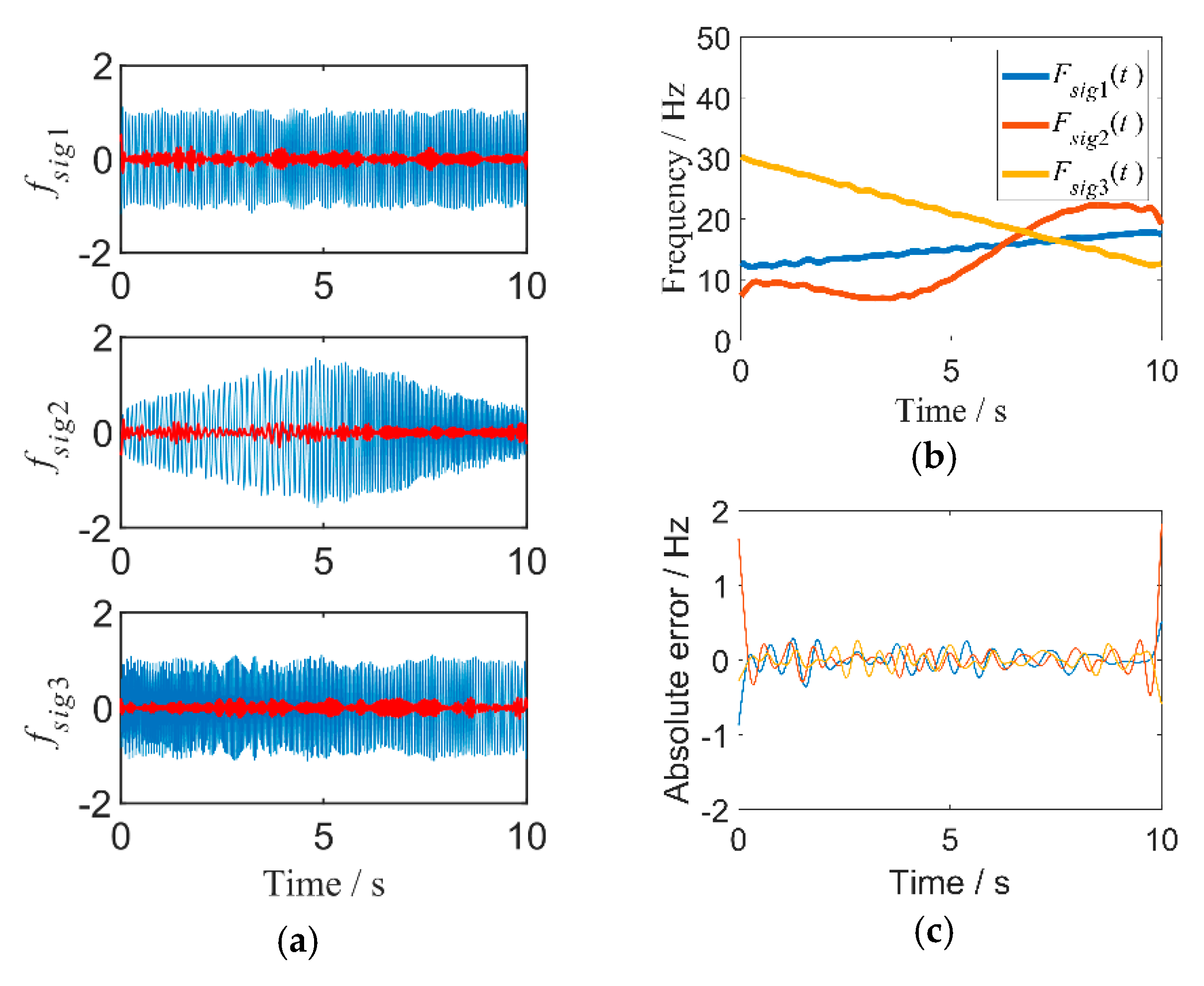
4.1. Method Validation

In this subsection, we used VSME to analyze a artificial signal, which is a intrawave amplitude modulated and frequency modulated signal. Artificial data generated from mathematical expression were calculated to evaluate the performance of VSME. All the calculation work was running in MATLAB R2016b.
The artificial signal contains a signal whose frequency increases linearly with time, a signal whose frequency decreases linearly with time, and a signal with time-varying frequency and amplitude, as shown in Equation (36).
f ( t ) = f s i g 1 ( t ) + f s i g 2 ( t ) + f s i g 3 ( t )
f s i g 1 ( t ) = cos ( 2 π ( 0.3 t 2 + 12 t + 0.6 ) )
f s i g 2 ( t ) = ( 0.4 cos ( 0.2 π t ) 1 ) × cos ( 2 π ( 5 ( sin π t 4 ) ) + 0.8 t 2 + 5 t )
f s i g 3 ( t ) = cos ( 2 π ( 0.9 t 2 + 30 t + 0.55 ) )
For signal frequency extraction, we used VSME and RPRG (Ridge Path Regrouping) [42] algorithm to compare the extraction effect. RPRG method is a novel non-parametric algorithm to extract IF from signal with overlapping components in time-frequency representation. Figure 2a is an image of a mixed signal f ( t ) , and Figure 2b shows the IF of original component signal f s i g 1 ( t ) , f s i g 2 ( t ) and f s i g 3 ( t ) . The IF of component signal extracted by RPRG is shown in Figure 2e. It is observed that at the intersection of IF of three component signals, an abnormal shape is generated. Using VSME to extract the IF of mode component, we can get a better result than RPRG, as shown in Figure 2c. To quantify the separation effect of VSME and RPRG on mixed signals f ( t ) , Figure 2d,f show the absolute error between the estimated IF extracted by the two methods and the true IF.
To compare with different methods, we employed VSME and VMD to extract the mode components of original signal f ( t ) . The red line shown in Figure 3a represents the estimated three mode components, and the blue line represents the absolute error between the estimated modes and the original modes in the vicinity of plane y = 0 . The absolute error range is less than 0.05, and the relative error is not more than 1%. By comparing Figure 3a,b, we can conclude that the VMD algorithm has a poor separation result on mixed signals f ( t ) .
In this paper, the performance of VSME is studied by adding white noise to the artificial signal f ( t ) . The signal-to-noise ratio (SNR) is defined as:
S N R = 10 log 10 ( P x / P ε )
where P x represents the energy of noiseless signal, and P ε is the energy of the noise signal. The mean value of ε ( t ) is 0, and its variance σ ε 2 = 1 .
Figure 4 and Figure 5 analyze the mode extraction performance of VSME algorithm for mixed signal f ( t ) , when the SNR is 12 dB and 18 dB respectively. The results show that the algorithm is effective when the SNR is 18 dB; when the SNR is lower than 12 dB, the IF has obvious fluctuation effect in the time domain, as shown in Figure 4c. We will continue to optimize the algorithm in the future work, aiming at extract mode components more accurately in low SNR condition.
The root mean squared error (RMSE) is used to measure the filtered signal error under different SNR levels, which is defined as:
R M S E = 1 m 1 m ( g ^ k ( t ) g k ( t ) )
where g ^ k ( t ) is k t h estimated signal component, and g k ( t ) is the true signal.
The 2-Norm error expression is:
L 2 = g ^ k ( t ) g k ( t ) 2 g k ( t ) 2
where · is the 2-Norm of the function, and g ^ k ( t ) is the k t h estimated component signal.
Figure 6 shows the calculated values of RMSE and 2-Norm of the estimated component signal under different SNR conditions. When the SNR is 12 dB, the values of RMSE is less than 0.02, and 2-Norm does not exceed 0.2; when the SNR is more than 20 dB, the values of RMSE and 2-Norm tend to decline steadily and are less than 0.05.
In this section, we simplify the problem by extracting the interested component of a simulated signal, and verify the reliability of VSME algorithm. It uses the same mode definition as VMD, especially using Wiener filter to detect the signal mode. The difference is that the number of modal components is determined before VMD calculation, and VSME only extracts the mode of interest through its center frequency. VMD uses iterative method to determine all modal components, and the calculation can be stopped until all modes reach the optimal response. Therefore, this property of VMD reduces the convergence rate of calculation. In addition, the performance of VMD is greatly impacted by the number of modal components, which is given at the beginning of calculation. However, VSME only searches for the component of interest, thus its computational efficiency is not affected by modal number. Without setting the property of specific mode in advance, VSME can extract the interested mode component from a mixed signal, such as the defect signal detection of buried pipeline. The results showed that VSME can achieve better performance and higher calculation efficiency.

4.2. Experimental Results

4.2.1. Experimental Setup

To verify the effectiveness of proposed VSME method for pipeline detection, an experiment was carried out using the experimental equipment shown in Figure 7 The experimental device consists of cross array with five magnetic sensor elements, a data acquisition card, a GPS positioning system, and a data acquisition system. Sampling frequency of the experimental instrument is 1 kHz, and each sensor is three-axis differential output. Testing equipment can locate these lines and accurately measure the size and specific location of all defects.
Array element adopts the triaxial sensor of Tunnel Magnetoresistance (TMR) produced by MultiDimension Technology, and the model is TMR2905. To prevent the acquisition system from interfering with the array, we use digital signal communication to transmit signals by two Universal Serial Bus cables. Data acquisition system is responsible for receiving signals for display, storage, and related control functions. Global Positioning System (GPS) is integrated into the experimental instrument for precise positioning and trajectory tracking. Its P3 mobile terminal and I70 carry out differential conversion of satellite signals through digital radio communication with accuracy up to centimeter level, which uses the GPS Fix Data in the current international NMEA0183 standard format for conversion and preservation. GPS data can be directly converted into Keyhole Markup Language format file through Google map API, which can directly display the actual map, and can mark the location of pipe body damage abnormally.
The laboratory experimental pipeline is made of Q235 steel material with a wall thickness of 3 mm, and a diameter of 75 mm. We fabricated six defects at different locations of the pipe to study the magnetic anomaly signals of different defects, as shown in Figure 8.
The shapes of these six defects are axial crack, transverse crack, square groove, through hole, blind hole, and 45-degree crack in turn, as shown in Figure 9. There were four different lift-off distance detection experiments, which are 0.5 m, 1.0 m, 1.5 m and 2.0 m, respectively.

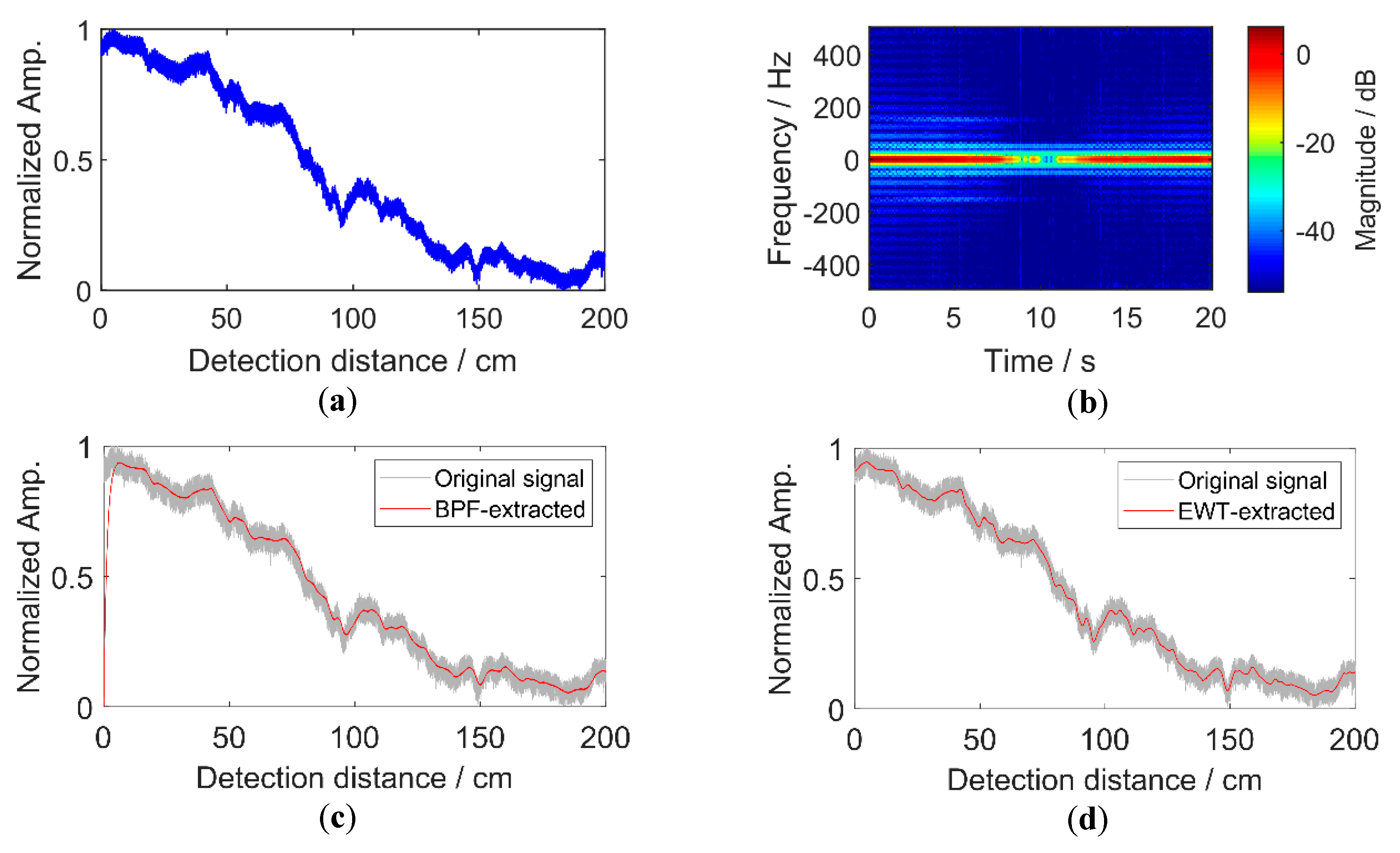
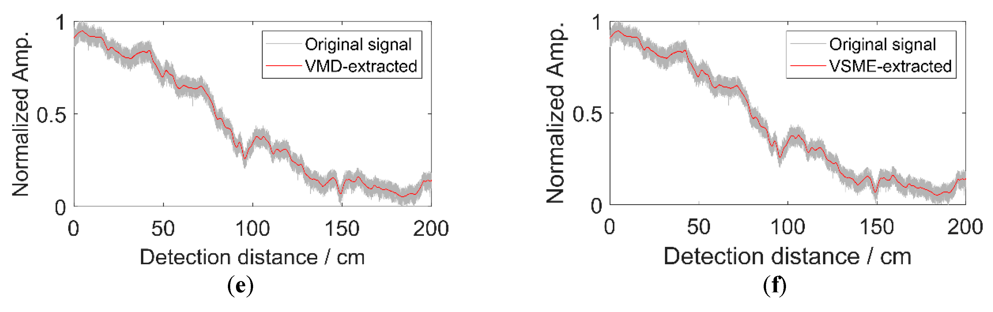
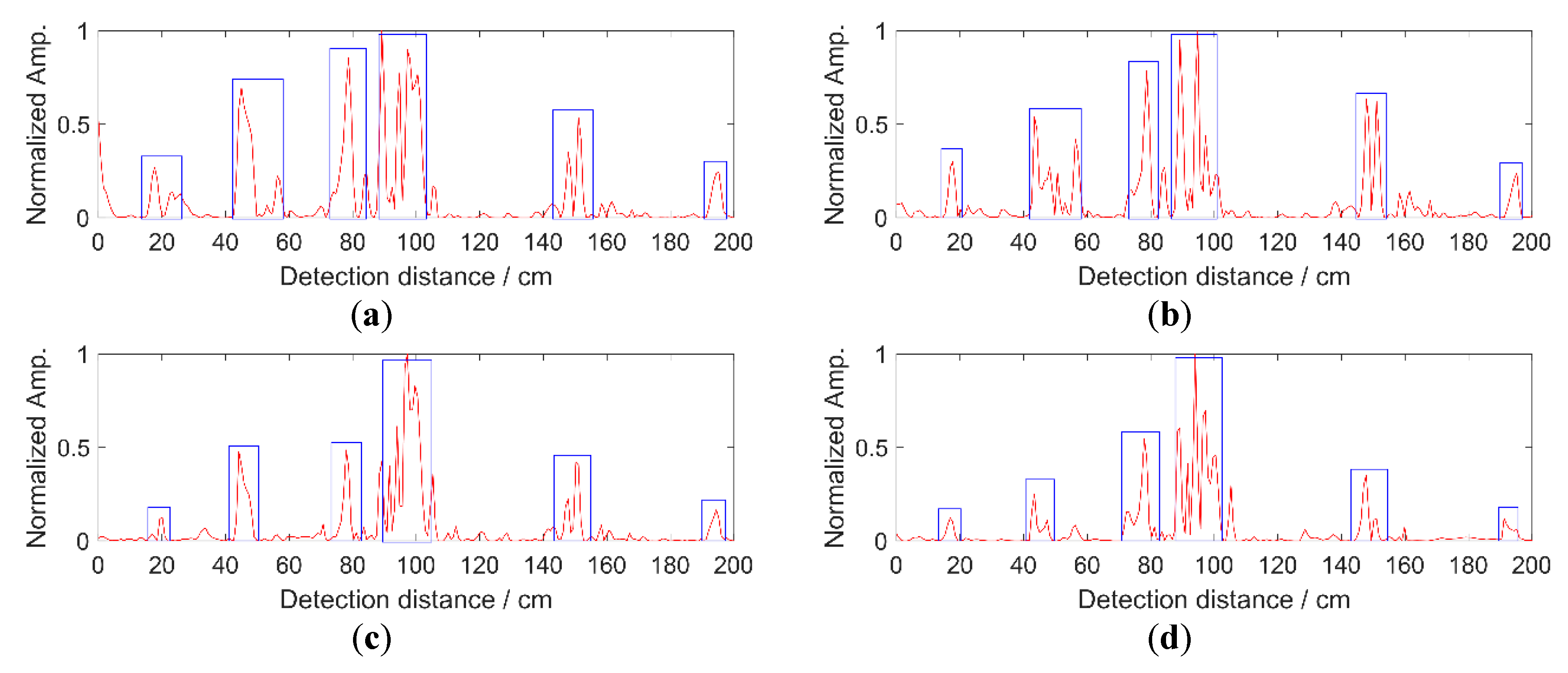
4.2.2. Results Analysis

Buried pipelines are affected by external factors, thus the algorithm for extracting defect signals should have a certain anti-noise performance, and it should also have the ability to extract abnormal signal of subtle change. Therefore, we compare the performance of band-pass filter (BPF), EWT, VMD, and VSME for pipeline defect signals.
Before extracting the pipeline defect signal in original signal, as shown in Figure 10a, we first use STFT to carry out time-frequency spectrum analysis of the signal. Figure 10b shows that the main energy of acquired signal is concentrated in the low-frequency component, and the frequency spectrum changes abnormally in the middle of detected pipeline. According to the actual pipeline being tested, as shown in Figure 9, the position of through hole defect in pipeline is just detected at about 10th second of constant speed detection, where pipeline damage is relatively serious. This situation is usually not effective for the BPF method, and its response contains some additional fluctuations, which increase with the increase of noise level. Figure 10d–f show that analysis results of EWT, VMD, and VSME are satisfactory, and it is difficult to identify the subtle differences manually. In the following analysis, we use quantitative indicators to measure the filtering effect.
Considering the length of article, only one group data of analysis figures was listed, and other groups of data gave the calculation results. To analyze the accuracy of mentioned algorithms in extracting MAD signal, frequency band of magnetic anomaly signal is obtained from the defect signal of experimental pipeline, and then detection results are analyzed statistically. We use SNR, normalized cross correlation coefficient (NCCC), and root mean square error (RMSE) to evaluate the performance difference between VME detectors and other techniques. The calculation equations of the two indexes are in Equations (40) and (41), and the NCCC is as follows:
N C C C = n = 0 N 1 x ^ ( n ) x ( n ) [ n = 0 N 1 x ^ 2 ( n ) n = 0 N 1 x 2 ( n ) ] 1 / 2
where x ^ ( n ) is filtered output signal, x ( n ) is input signal, and N is signal dimension. The three mentioned indexes were calculated for Figure 11, and the average value is shown in Table 2.
To further evaluate the detection effect of pipeline defects at different lift-off distances, the SNR, RMSE, and NCCC of defect signals were computed using these algorithms. Figure 11 plots the evaluation indicators for the six sets of data, which are obtained at different lift-off distances. SNR of extracted defect signal gradually decreases as the lift-off distance increases, as shown in Figure 11a. The performance of VSME is slightly higher than VMD and EWT, but significantly higher than BPF. RMSE of the VSME-processed signal is generally lower than the other three methods, indicating that the proposed algorithm is more reliable, as shown in Figure 11b. When the lift-off distance increased from 0.5 m to 2 m, the value of RMSE showed a trend of increasing first and then decreasing. Through experimental analysis, when the lift-off distance is 1 m–1.5 m, the excessive RMSE fluctuation is due to the joint effect of the pipeline magnetic field signal and the surrounding interference, which leads to the instability of the magnetic field. As the lift-off height increases, the pipeline magnetic field signal weakens, thus the value of RMSE decreases. Figure 11c shows the NCCC, the performance of BPF is the worst, and VSME is slightly better than the other two methods. The analysis of the mentioned three filtering indicators shows that the VSME algorithm has good performance in the extraction of pipeline defect signals.
Calculation time of the same data set is an important index to measure algorithm. To compare the computational complexity of different algorithms, average time required to extract the MAD signal from the 100,000 sample points of experimental data is given in Table 3. According to the table, the calculation time of VSME is less than one-tenth that of VMD and EWT, and it can be compared with the computational complexity of BPF. Results showed that VSME has a good performance by evaluating the index of filtered experimental data.
Computational time for processing a segment of 100,000 samples (100 s) of acquired signal (in second). Computing platform adopts DELL-EQVS5M4, the hardware configuration is Intel (R) core (TM) i5-4430 CPU @ 3.0GHz and the memory is 8.0 GB. The system version is Windows 10 professional, and we use Matlab 2016b as signal processing software.
Comparing defect signals at different lift-off distances, we transformed the extracted MAD signal into a normalized gradient energy operator. By analyzing the test data of pipeline in laboratory, it is found that with the increase of the lift-off distance, the signal of the less damaged location becomes weaker. Six defects are easily detected when the lift-off distance is 0.5 m, as shown in Figure 7b. When lift-off distance is 2.0 m, six defects can still be detected. However, the signal with larger damage degree has a certain submergence effect on the position with smaller damage degree. Figure 12d shows that the signals are weak at the axial crack and 45-degree crack positions.
In this section, we concentrate on the performance of VSME in extracting MAD signals of pipeline defects. As mentioned, variational theory can provide effective solutions for pipeline defect signal extraction. Herein, we used and VSME to extract pipeline defect signals, and compared with BPF, EWT, and VMD. To ensure the performance of MAD signal extraction, we randomly selected six sets of experimental data, and extracted the MAD of defect signals by four algorithms on the same computing platform for several times. Then, the acquired MAD signals were evaluated by calculating the cross correlation coefficients with the reference pipeline defect signals. The results showed that VSME has certain advantages.

5. Conclusions

In the paper, we present a novel algorithm of extracting a specific mode component for non-contact inspection of pipeline defects. The proposed VSME is based on the fact that a wide-band signal can be converted into a narrow-band signal by demodulation method. Then, the problem of wide-band signal decomposition is expressed as an optimal demodulation problem, which can be solved by an improved ADMM. This algorithm does not need a parametric model, which makes it more suitable for practical problems. To verify the performance of VSME, we used this algorithm to analyze a complex simulation signal. Simulation results showed that VSME is more effective than VMD and EWT in extracting a specific mode signal, even in the case of modes overlap severely. Finally, we applied this method to the actual pipeline defect detection, and compared the detection results at different lift-off distances, which showed that it has a better anti-noise performance. Further work will be focused on improving the robustness of VSME in separating severely crossed component signals and on the applications of pipeline detection in more complex environment.

Author Contributions

Methodology, validation, and writing—original draft preparation, H.J.; writing—review and editing, and supervision, X.W.; validation, investigation, and data curation, Y.Z. All authors have read and agreed to the published version of the manuscript.

Funding

This research was funded by the National Key Research and Development Program of China, grant number 2017YFC0805005-1, and the Science and Technology Program of Beijing Municipal Education Commission, grant number KZ201810005009.

Conflicts of Interest

The authors declare no conflict of interest.

References

  1. Cataldo, A.; Cannazza, G.; De Benedetto, E.; Giaquinto, N. A new method for detecting leaks in underground water pipelines. IEEE Sens. J. 2011, 12, 1660–1667. [Google Scholar] [CrossRef]
  2. Vanaei, H.R.; Eslami, A.; Egbewande, A. A review on pipeline corrosion, in-line inspection (ILI), and corrosion growth rate models International. J. Press. Vessel. & Pip. 2017, 149, 43–54. [Google Scholar]
  3. Duisterwinkel, E.H.; Talnishnikh, E.; Krijnders, D.; Wörtche, H.J. Sensor motes for the exploration and monitoring of operational pipelines. IEEE Trans. Instrum. Meas. 2018, 67, 655–666. [Google Scholar] [CrossRef]
  4. Quarini, J.; Shire, S. A Review of Fluid-Driven Pipeline Pigs and their Applications. Proc. Inst. Mech. Eng.-Part E 2007, 221, 1–10. [Google Scholar] [CrossRef]
  5. Pham, H.Q.; Tran, B.V.; Doan, D.T.; Le, V.S.; Pham, Q.N.; Kim, K.; Kim, C.; Terki, F.; Tran, Q.H. Highly sensitive planar hall magnetoresistive sensor for magnetic flux leakage pipeline inspection. IEEE Trans. Magn. 2018, 54, 1–5. [Google Scholar] [CrossRef]
  6. Civera, M.; Fragonara, L.Z.; Surace, C. Video processing techniques for the contactless investigation of large oscillations. J. Phys. Conf. Ser. IOP Publ. 2019, 1249, 012004. [Google Scholar] [CrossRef]
  7. Civera, M.; Zanotti Fragonara, L.; Surace, C. An experimental study of the feasibility of phase-based video magnification for damage detection and localisation in operational deflection shapes. Strain 2020, 56, e12336. [Google Scholar] [CrossRef]
  8. Li, Y.; Yan, B.; Li, D.; Li, Y.; Zhou, D. Gradient-field pulsed eddy current probes for imaging of hidden corrosion in conductive structures. Sens. & Actuators A Phys. 2016, 238, 251–265. [Google Scholar]
  9. Jarvis, R.; Cawley, P.; Nagy, P.B. Current deflection NDE for the inspection and monitoring of pipes. NDT & E Int. 2016, 81, 46–59. [Google Scholar]
  10. Honarvar, F.; Salehi, F.; Safavi, V.; Mokhtari, A.; Sinclair, T. Ultrasonic monitoring of erosion/corrosion thinning rates in industrial piping systems. Ultrasonics 2013, 53, 1251–1258. [Google Scholar] [CrossRef]
  11. Hu, B.; Yu, R.; Liu, J. Experimental study on the corrosion testing of a buried metal pipeline by transient electromagnetic method. Anti-Corros. Methods Mater. 2016, 63, 262–268. [Google Scholar] [CrossRef]
  12. Haith, M.I.; Huthwaite, P.; Lowe, M.J. Defect characterisation from limited view pipeline radiography. NDT & E Int. 2017, 86, 186–198. [Google Scholar]
  13. Chongchong, L.; Lihong, D.; Haidou, W.; Guolu, L.; Binshi, X. Metal magnetic memory technique used to predict the fatigue crack propagation behavior of 0.45% C steel. J. Magn. Magn. Mater. 2016, 405, 150–157. [Google Scholar] [CrossRef]
  14. Aydin, U.; Rasilo, P.; Singh, D.; Lehikoinen, A.; Belahcen, A.; Arkkio, A. Coupled magneto-mechanical analysis of iron sheets under biaxial stress. IEEE Trans. Magn. 2015, 52, 1–4. [Google Scholar] [CrossRef] [Green Version]
  15. Dubov, A.; Kolokolnikov, S. The metal magnetic memory method application for online monitoring of damage development in steel pipes and welded joints specimens. Weld. World 2013, 57, 123–136. [Google Scholar] [CrossRef]
  16. Augustyniak, M.; Usarek, Z. Discussion of Derivability of Local Residual Stress Level from Magnetic Stray Field Measurement. J. Nondestruct. Eval. 2015, 34, 21. [Google Scholar] [CrossRef] [Green Version]
  17. Liu, Z.; Pang, H.; Pan, M.; Wan, C. Calibration and Compensation of Geomagnetic Vector Measurement System and Improvement of Magnetic Anomaly Detection. IEEE Geosci. & Remote Sens. Lett. 2016, 13, 447–451. [Google Scholar]
  18. Sheinker, A.; Moldwin, M.B. Magnetic anomaly detection (MAD) of ferromagnetic pipelines using principal component analysis (PCA). Meas. Sci. & Technol. 2016, 27, 45104. [Google Scholar]
  19. Buhari, M.D.; Tian, G.Y.; Tiwari, R. Microwave-Based SAR Technique for Pipeline Inspection Using Autofocus Range-Doppler Algorithm. IEEE Sens. J. 2018, 19, 1777–1787. [Google Scholar] [CrossRef] [Green Version]
  20. Fallahpour, M.; Case, J.T.; Ghasr, M.T.; Zoughi, R. Piecewise and Wiener filter-based SAR techniques for monostatic microwave imaging of layered structures. IEEE Trans. Antennas Propag. 2013, 62, 282–294. [Google Scholar] [CrossRef]
  21. Gilmore, C.; Jeffrey, I.; Lovetri, J. Derivation and comparison of SAR and frequency-wavenumber migration within a common inverse scalar wave problem formulation. IEEE Trans. Geosci. Remote Sens. 2006, 44, 1454–1461. [Google Scholar] [CrossRef]
  22. Winters, D.W.; Van Veen, B.D.; Hagness, S.C. A sparsity regularization approach to the electromagnetic inverse scattering problem. IEEE Trans. Antennas Propag. 2009, 58, 145–154. [Google Scholar] [CrossRef] [PubMed] [Green Version]
  23. De Zaeytijd, J.; Franchois, A.; Eyraud, C.; Jean-Michel, G. Full-wave three-dimensional microwave imaging with a regularized Gauss-Newton method-Theory and experiment. IEEE Trans. Antennas Propag. 2007, 55, 3279–3292. [Google Scholar] [CrossRef]
  24. De Zaeytijd, J.; Franchois, A.; Geffrin, J. A new value picking regularization strategy—Application to the 3-D electromagnetic inverse scattering problem. IEEE Trans. Antennas Propag. 2009, 57, 1133–1149. [Google Scholar] [CrossRef]
  25. Sheinker, A.; Ginzburg, B.; Salomonski, N.; Dickstein, P.A.; Frumkis, L.; Kaplan, B. Magnetic Anomaly Detection Using High-Order Crossing Method. IEEE Trans. Geosci. & Remote Sens. 2012, 50, 1095–1103. [Google Scholar]
  26. Sheinker, A.; Salomonski, N.; Ginzburg, B.; Frumkis, L.; Kaplan, B. Magnetic anomaly detection using entropy filter. Meas. Sci. & Technol. 2008, 19, 45205. [Google Scholar]
  27. Zhou, H.; Pan, Z.; Zhang, Z. Magnetic Anomaly Detection with Empirical Mode Decomposition Trend Filtering. IEICE Trans. Fundam. Electron. Commun. Comput. Sci. 2017, 2503–2506. [Google Scholar] [CrossRef]
  28. Huang, N.E.; Shen, Z.; Long, S.R.; Wu, M.C.; Shih, H.H.; Zheng, Q.; Yen, N.; Tung, C.C.; Liu, H.H. The empirical mode decomposition and the Hilbert spectrum for nonlinear and non-stationary time series analysis. Proc. Math. Phys. & Eng. Sci. 1998, 454, 903–995. [Google Scholar]
  29. Wu, Z.; Huang, N.E. Ensemble empirical mode decomposition: A noise-assisted data analysis method. Adv. Adapt. Data Anal. 2009, 1, 1–41. [Google Scholar] [CrossRef]
  30. Yeh, J.R.; Shieh, J.S.; Huang, N.E. Complementary Ensemble Empirical Mode Decomposition: A Novel Noise Enhanced Data Analysis Method. Adv. Adapt. Data Anal. 2010, 2, 135–156. [Google Scholar] [CrossRef]
  31. Gilles, J. Empirical Wavelet Transform. IEEE Trans. Signal Proc. 2013, 61, 3999–4010. [Google Scholar] [CrossRef]
  32. Chen, S.; Dong, X.; Peng, Z.; Zhang, W.; Meng, G. Nonlinear Chirp Mode Decomposition: A Variational Method. IEEE Trans. Signal Process. 2017, 65, 6024–6037. [Google Scholar] [CrossRef]
  33. Dragomiretskiy, K.; Zosso, D. Variational Mode Decomposition. IEEE Trans. Signal Process. 2014, 62, 531–544. [Google Scholar] [CrossRef]
  34. Ma, W.; Yin, S.; Jiang, C.; Zhang, Y. Variational mode decomposition denoising combined with the Hausdorff distance. Rev. Sci. Instrum. 2017, 88, 35109. [Google Scholar] [CrossRef] [PubMed]
  35. Nazari, M.; Sakhaei, S.M. Variational Mode Extraction: A New Efficient Method to Derive Respiratory Signals from ECG. IEEE J. Biomed. Health Inf. 2018, 22, 1059–1067. [Google Scholar] [CrossRef] [PubMed]
  36. Wang, S.; Chen, X.; Cai, G.; Chen, B.; Li, X.; He, Z. Matching Demodulation Transform and SynchroSqueezing in Time-Frequency Analysis. IEEE Trans. Signal Process. 2014, 62, 69–84. [Google Scholar] [CrossRef]
  37. Boyd, S.; Parikh, N.; Chu, E.; Peleato, B.; Eckstein, J. Distributed Optimization and Statistical Learning via the Alternating Direction Method of Multipliers. Found. & Trends® Mach. Learn. 2010, 3, 1–122. [Google Scholar]
  38. Tejero, C.E.J.; Sallares, V.; Ranero, C.R. Appraisal of instantaneous phase-based functions in adjoint waveform inversion. IEEE Trans. Geosci. Remote Sens. 2018, 56, 5185–5197. [Google Scholar] [CrossRef] [Green Version]
  39. Mcneill, S.I. Decomposing a signal into short-time narrow-banded modes. J. Sound Vib. 2016, 373, 325–339. [Google Scholar] [CrossRef]
  40. Pustelnik, N.; Borgnat, P.; Flandrin, P. Empirical mode decomposition revisited by multicomponent non-smooth convex optimization. Signal Process. 2014, 102, 313–331. [Google Scholar] [CrossRef]
  41. Goldstein, T.; O’Donoghue, B.; Setzer, S. Fast alternating direction optimization methods. SIAM J. Imaging Sci. 2014, 7, 1588–1623. [Google Scholar] [CrossRef] [Green Version]
  42. Chen, S.; Dong, X.; Xing, G.; Peng, Z.K.; Zhang, W.; Meng, G. Separation of overlapped non-stationary signals by ridge path regrouping and intrinsic chirp component decomposition. IEEE Sens. J. 2017, 17, 5994–6005. [Google Scholar] [CrossRef]
Figure 1. Description of demodulation procedure (Purple line: instantaneous frequency of the original FM signal; red line: instantaneous frequency of the forward demodulated signal; blue line: instantaneous frequency of the backward modulation signal.). Before demodulation, the spectrum of original signal is distributed around the frequency f c + φ ( u ) / 2 π .
Algorithms 13 00105 g001
Figure 2. Frequency analysis of estimated component signal. (a) Original artificial signal. (b) Frequency of original component signal in time domain. (c) Frequency of estimated component signal extracted by RPRG. (d) Frequency of estimated component signal extracted by VSME. (e) Absolute error of estimated component signal frequency extracted by VSME. (f) Absolute error of estimated component signal frequency extracted by RPRG.
Algorithms 13 00105 g002
Figure 3. Analysis results. (a) The estimated modes by VSME (blue: estimated modes; red: estimation errors). (b) The estimated modes by VMD.
Algorithms 13 00105 g003
Figure 4. Analysis results with SNR = 12 dB. (a) The estimated modes by VSME. (b) Frequency of estimated component signal extracted by VSME. (c) Absolute error of estimated component signal frequency extracted by VSME.
Algorithms 13 00105 g004
Figure 5. Analysis results with SNR = 18 dB. (a) The estimated modes by VSME. (b) Frequency of estimated component signal extracted by VSME. (c) Absolute error of estimated component signal frequency extracted by VSME.
Algorithms 13 00105 g005
Figure 6. Error analysis under different SNR. (a) The values of RMSE; (b) the values of 2-Norm.
Algorithms 13 00105 g006
Figure 7. Laboratory experiment of pipeline inspection. (a) Picture of experimental setup, 1—Global positioning system, 2—Data Acquisition System, 3—Acquisition Card, 4—Magnetic Sensor; (b) Laboratory scheme design; (c) Field test; (d) Defect location.
Algorithms 13 00105 g007aAlgorithms 13 00105 g007b
Figure 8. Locations of defects in the laboratory pipeline.
Algorithms 13 00105 g008
Figure 9. Images of defects in the ferromagnetic pipeline. (a) The size of axial crack is 30 mm × 1 mm × 1 mm; (b) The size of axial crack is 1 mm × 20 mm × 1 mm; (c) The size of axial crack is 12 mm × 20 mm × 1 mm; (d) The diameter of through hole is 10 mm; (e) The diameter and depth of blind hole are 10 mm and 1 mm; (f) The size of 45-degree crack is 1 mm × 20 mm × 1 mm.
Algorithms 13 00105 g009aAlgorithms 13 00105 g009b
Figure 10. Analysis results for the Lab. 1 signal. (a) Acquired original magnetic field signal; (b) Fourier spectrum of original signal by STFT; (c) Pipeline defect signal extracted by band-pass filter; (d) Pipeline defect signal extracted by EWT; (e) Pipeline defect signal extracted by VMD; (f) Pipeline defect signal extracted by VSME.
Algorithms 13 00105 g010aAlgorithms 13 00105 g010b
Figure 11. Performance evaluation for the defect signals at different lift-off distances. (a) SNR plot, (b) RMSE plot, (c) NCCC plot.
Algorithms 13 00105 g011
Figure 12. Defect detection results of pipeline at different lift-off distances in laboratory. (a) Lift-off distance is 0.5 m; (b) Lift-off distance is 1.0 m; (c) Lift-off distance is 1.5 m; (d) Lift-off distance is 2.0 m. Six blue boxes from left to right are the defect locations on pipeline, which are axial crack, transverse crack, square groove, through hole, blind hole, and 45-degree crack in turn.
Algorithms 13 00105 g012
Table 1. Comparison of EMD, EWT, VMD and VSME.
ContentsEMDEWTVMDVSME
BasisSelf-adaptionPrior determinationPrior determinationSelf-adaption
FrequencyDifference: LocalConvolution: LocalDifference: GlobalConvolution: Global
CharacterizationEnergy-TimeEnergy-Time-FrequencyEnergy-Time-FrequencyEnergy-Time-Frequency
NonlinearYesYesYesYes
NonstationarityYesNoNoYes
Feature ExtractionYesDiscrete: No
Continuous: Yes
YesYes
Theoretical BasisEmpiricalComplete theoryComplete theoryComplete theory
Table 2. Mean and standard deviation (SD) of the three indexes used for comparing different algorithms.
AlgorithmsSNR/dBRMSENCCC
MSDMSDMSD
BPF2.230.200.150.100.810.46
EWT2.610.120.180.060.890.26
VMD3.080.890.110.680.940.16
VSME3.260.050.130.020.950.04
M is the mean and S D is the standard deviation of the filtered signal.
Table 3. Mean and standard deviation (SD) of calculation time.
AlgorithmBPFEMDVMDVSME
Mean/s5.69146.82108.3610.63
SD0.0416.788.291.08

