New Numerical Treatment for a Family of Two-Dimensional Fractional Fredholm Integro-Differential Equations

Abstract

In this paper, we present a robust algorithm to solve numerically a family of two-dimensional fractional integro differential equations. The Haar wavelet method is upgraded to include in its construction the Laplace transform step. This modification has proven to reduce the accumulative errors that will be obtained in case of using the regular Haar wavelet technique. Different examples are discussed to serve two goals, the methodology and the accuracy of our new approach.

1. Introduction

Wavelet on $\mathrm{I}\mathrm{R}$ is studied by many mathematicians to construct an orthonormal basis for $L^2\left[\mathrm{I}\mathrm{R}\right]$; see [1,2,3]. One of the common wavelets is the Haar wavelet on $\mathrm{I}\mathrm{R}$. In approximation theory, once we have these bases, we are ready to find approximate solutions for many of the applied problems such as in [4,5]. Let $u(x,t)$ be a function defined over $[0,1]\times [0,1]$, and let $k(x,t,y,\tau )$ be a continuous kernel; in addition, assume $0<\alpha <1$. In this work, we are interested in solving the two-dimensional fractional Fredholm integro-differential equation of the form:

$$D_t^{\alpha }u(x,t)=f(x,t)+{\int }_0^1{\int }_0^{1}k(x,t,y,\tau )u(y,\tau )dyd\tau ,$$

(1)

where $D_t^{\alpha }u\left(t\right)$ is the fractional derivative in the sense of Caputo definition.

Babolian and Shahsavaran [4] obtained a numerical solution of nonlinear Fredholm integral equations of the second kind using Haar wavelets. In addition, Aziz, Fayyaza, and Islama proposed in [6] a new method for the numerical solution of a one-dimensional nonlinear Fredholm and Volterra using Haar wavelets. This method is the extension of Aziz and Islama work in [7]. Moreover, Aziz, Khan, and Islama also found a numerical solution for the two-dimensional nonlinear integral equation by establishing a new method based on Haar wavelet. In addition, Rehman and Khan in [8] solved fractional differential equations using the Legendre wavelet method. Furthermore, Pedas and Tamme, in [9], used spline collocation methods for multi-term fractional differential equations. In [4], Shesha, Savitha, and Nargund used the Haar wavelet method for the numerical solution of a two-dimensional Fredholm integral equation of the second kind. After awhile, Cattani used Shannon wavelets for the solution of integro-differential equations [10].

In [5], Lepik provided a numerical solution for one-dimensional, fractional integral equations using the Haar wavelet method. A similar approach can be done by replacing functions of one variable by functions of two variables. In this paper, we find numerical solutions for the fractional integro-differential Equation (1) using the Haar wavelet method (HWM); then, we use a modified approach with the help of Laplace transform to solve the same equation. The examples we provide show the efficiency of the second method comparing with the HWM.

2. Preliminaries and Basic Concepts

2.1. Fractional Derivative

There are many definitions that describe the fractional derivative. Here, we use Caputo approach which is defined as follows:

Definition 1.

(Caputo derivative). [11] The fractional derivative of $f\left(x\right)$ in the Caputo sense is defined by

$$D_x^{\alpha }f\left(x\right)=\frac{1}{\mathsf{\Gamma }(n-\alpha )}{\int }_0^x{f}^{\left(n\right)}\left(t\right){(x-t)}^{n-\alpha -1}dtn\in \mathrm{I}\mathrm{N},n-1<\alpha <n.$$

(2)

It is worth mentioning that a Caputo derivative allows traditional initial and boundary conditions to be included in the formulation of the problem [12] as well as the derivative of the constant being zero. For more information and properties about Caputo derivative, we encourage the reader to see [11,13,14,15].

2.2. Laplace Transform

Definition 2.

We denote the Laplace transform of a function $f\left(t\right)$ by $F\left(s\right)$, which is defined as

$$F\left(s\right)=\mathcal{L}\left[f\left(t\right)\right]\left(s\right)={\int }_0^{\infty }{e}^{-st}f\left(t\right)dt.$$

(3)

Lemma 1.

The Laplace of the Caputo derivative is given by

$$\mathcal{L}\left[D_t^{\alpha }f\left(t\right)\right]\left(s\right)=s^{\alpha }F\left(s\right)-\sum _{k=0}^{n-1}{s}^{\alpha -k-1}{f}^{\left(k\right)}\left(0\right).$$

(4)

Definition 3.

A function f on $0\le t<\infty$ is said to be exponentially bounded if it satisfies an inequality of the form

$$\left|f\left(t\right)\right|\le M{e}^{ct},$$

for some real constants $M>0$ and c, for all sufficiently large t.

Theorem (3.1) given in [16] shows that one can take the Laplace operator over fractional differential equations if the homogeneous part is exponentially bounded. A modification of this mentioned theorem will be adjusted to fit with the proposed Fredholm equation as follows:

Theorem 1.

[16] Assume Equation (1) has a unique continuous solution $u(x,t)$. If $f(x,t)$ and $k(x,t,w,y)$ are continuous for $x,t,w,y\in [0,1]$ and exponentially bounded in t, then $u(x,t)$ and its Caputo derivative are exponentially bounded in t, and their Laplace transforms exist in t.

As a corollary of this theorem and the Fubini’s Theorem, we have the following result

Corollary 1.

Let $k(x,t,w,y)$ be continuous for $0\le x,t,y,w\le 1$ and of exponential order in t. If

$$f(x,t)={\int }_0^1{\int }_0^{1}k(x,t,y,w)dydw,for0\le x,t\le 1,$$

then the Laplace transform of $t\mapsto f(x,t)$ exists and $F(x,s)={\int }_0^1{\int }_0^{1}K(x,s,y,w)dydw$, where $K(x,s,y,w)$ is the Laplace transform of $t\mapsto k(x,t,y,w)$.

2.3. Haar Wavelet

Wavelet analysis is the tool to construct an orthonormal basis for $L^2\left[\mathbb{R}\right]$. One of the common wavelet bases is the Haar basis. In fact, for any $i=2,3,4,\dots$ there are unique $j\ge 0$ and $0\le k\le 2^j-1$ such that $i=2^j+k+1$. Hence, we define the family $\left\{h_i\right\}$ by

$$h_1\left(x\right)=\left\{\begin{array}{cc}1,\hfill & 0\le x<1\hfill \\ 0,\hfill & \mathrm{elsewhere}\hfill \end{array}\right..$$

(5)

and

$$h_i\left(x\right)={\psi }_{j,k}\left(x\right)=2^{j/2}\psi (2^{j}x-k),fori=2,3,4,\dots$$

where

$$\psi \left(x\right)=\left\{\begin{array}{cc}1,\hfill & 0\le x<\frac{1}{2}\hfill \\ -1,\hfill & \frac{1}{2}\le x<1\hfill \\ 0,\hfill & \mathrm{elsewhere}\hfill \end{array}\right..$$

The family $\left\{h_i\right\}$ defines an orthonormal basis for $L^2[0,1]$—that is, any $f\left(x\right)$ in $L^2[0,1]$ has the expansion $f\left(x\right)={\sum }_{i=1}^{\infty }{a}_i{h}_i\left(x\right)$. For approximation purposes, the resolution level J is the maximum value for j in $i=2^j+k+1$. Thus, for given resolution level J, we define the truncated series expansion of $f\left(x\right)$ by

$$f\left(x\right)\approx \sum _{i=1}^{2^{J+1}}{a}_i{h}_i\left(x\right)$$

where $i=2^j+k+1$, $j=0,1,2,3,\dots ,J$, and $0\le k\le 2^j-1$. In

Table 1. Index computations for Haar basis function at $J=3$.

j	0	1	1	2	2	2	2	3	3	3	3	3	...	3
k	0	0	1	0	1	2	3	0	1	2	3	4	...	7
$i=2^j+k+1$	2	3	4	5	6	7	8	9	10	11	12	13	...	16

, we compute explicitly the corresponding values of j, k, and i for resolution level $J=3$.

Since we are dealing with both of $u\left(x\right)$ and its derivative $u^{\prime }\left(x\right)$ in differential equations, we will introduce the integrating Haar functions [5] by

$$p_i\left(x\right)={\int }_0^x{h}_i\left(x\right)dx=\left\{\begin{array}{cc}x-\frac{k}{2^j},\hfill & \frac{k}{2^j}\le x<\frac{k+0.5}{2^j}\hfill \\ \frac{k+1}{2^j}-x,\hfill & \frac{k+0.5}{2^j}\le x<\frac{k+1}{2^j}\hfill \\ 0,\hfill & \mathrm{elsewhere}\hfill \end{array}\right..$$

(6)

It follows that, if we approximate $u^{\prime }\left(x\right)\approx {\sum }_{i=1}^{2^{J+1}}{a}_i{h}_i\left(x\right)$, then we have $u\left(x\right)-u\left(0\right)\approx {\sum }_{i=1}^{2^{J+1}}{a}_i{p}_i\left(x\right)$

3. Haar Wavelet Method and Laplace Haar Wavelet Method

In this section, we propose the methodology of both the Haar wavelet method and the Laplace Haar wavelet method to find a numerical solution to the suggested two-dimensional integro-differential equation

$$D_t^{\alpha }u(x,t)=f(x,t)+{\int }_0^1{\int }_0^{1}k(x,t,y,\tau )u(y,\tau )dyd\tau$$

(7)

subject to the initial condition

$$u(x,0)=0,$$

(8)

where $0<\alpha <1$, and $D_t^{\alpha }u(x,t)$ is the Caputo derivative.

3.1. Haar Wavelet Method (HWM)

We summarize the Haar wavelet approach in the following steps.

Step 1: After we determine the level of resolution J to approximate $u(x,t)$, we assume

$$\frac{\partial }{\partial t}u(x,t)\approx \sum _{i=1}^{2^{J+1}}\sum _{j=1}^{2^{J+1}}{a}_{ij}{h}_i\left(x\right)h_j\left(t\right),$$

(9)

where $\left\{a_{ij}\right\}$ are to be determined. Using the initial condition in (8) and integrating with respect to t over $[0,t]$, one can write

$$u(x,t)\approx \sum _{i=1}^{2^{J+1}}\sum _{j=1}^{2^{J+1}}{a}_{ij}{h}_i\left(x\right)p_j\left(t\right).$$

It follows that the integral term can be estimated by

$${\int }_0^1{\int }_0^{1}k(x,t,y,\tau )u(y,\tau )dyd\tau \approx \sum _{i=1}^{2^{J+1}}\sum _{j=1}^{2^{J+1}}{a}_{ij}{\int }_0^1{\int }_0^{1}k(x,t,y,\tau )h_i\left(y\right)p_j\left(\tau \right)dyd\tau$$

Step 2: Now, to estimate the term $D_t^{\alpha }u(x,t)$, we plug Equation (9) into the definition of $D_t^{\alpha }u(x,t)$ to get

$$\begin{array}{cc}\hfill D_t^{\alpha }u(x,t)& =\frac{1}{\mathsf{\Gamma }(1-\alpha )}{\int }_0^t\frac{\partial }{\partial t}u(x,t){(t-\tau )}^{-\alpha }d\tau \hfill \\ \hfill & \approx \frac{1}{\mathsf{\Gamma }(1-\alpha )}\sum _{i=1}^{2^{J+1}}\sum _{j=1}^{2^{J+1}}{a}_{ij}{h}_i\left(x\right){\int }_0^t{h}_j\left(\tau \right){(t-\tau )}^{-\alpha }d\tau \hfill \end{array}$$

Step 3: Use the results of step (1) and (2) to obtain the equation

$$\frac{1}{\mathsf{\Gamma }(1-\alpha )}\sum _{i=1}^{2^{J+1}}\sum _{j=1}^{2^{J+1}}{a}_{ij}{h}_i\left(x\right){\int }_0^t{h}_j\left(\tau \right){(t-\tau )}^{-\alpha }d\tau =f(x,t)+\sum _{i=1}^{2^{J+1}}\sum _{j=1}^{2^{J+1}}{a}_{ij}{\int }_0^1{\int }_0^{1}k(x,t,y,\tau )h_i\left(y\right)p_j\left(\tau \right)dyd\tau$$

Use the equally distance nodes $x_m=\frac{m-0.5}{2^{J+1}}$ and $t_n=\frac{n-0.5}{2^{J+1}}$ to construct the system:

$$\begin{array}{cc}\hfill \frac{1}{\mathsf{\Gamma }(1-\alpha )}\sum _{i=1}^{2^{J+1}}\sum _{j=1}^{2^{J+1}}{a}_{ij}{h}_i\left(x_m\right){\int }_0^{t_n}{h}_j\left(\tau \right){(t_n-\tau )}^{-\alpha }d\tau & =f(x_m,t_n)\hfill \\ \hfill & +\sum _{i=1}^{2^{J+1}}\sum _{j=1}^{2^{J+1}}{a}_{ij}{\int }_0^1{\int }_0^{1}k(x_m,t_n,y,\tau )h_i\left(y\right)p_j\left(\tau \right)dyd\tau \hfill \end{array}$$

for $m,n=1,2,3,\dots ,2^{J+1}$.

The wavelet coefficients $a_{ij}$ are obtained by solving the above the $2^{J+1}\times 2^{J+1}$ system of equations.

3.2. Laplace Haar Wavelet Method (LHWM)

In this section, we summarize the methodology of Laplace Haar wavelet method to the two-dimensional integro-differential Equation (7), where we consider in this approach the more general case, for $n-1<\alpha <n$ and initial conditions

$$u(x,0)=u_0\left(x\right),\frac{\partial }{\partial t}u(x,0)=u_1\left(x\right),\dots ,\frac{{\partial }^{n-1}}{\partial t^{n-1}}u(x,0)=u_{n-1}\left(x\right)$$

which can be reached in the following steps.

Step 1. Determine the level of resolution J.

Step 2. Applying the Laplace transform to Equation (7), use Lemma 1, Corollary 1, and use the initial conditions $u_0\left(x\right)=u(x,0)$, $u_1\left(x\right)=\frac{\partial }{\partial t}u(x,0)$,..., $u_{n-1}\left(x\right)=\frac{{\partial }^{n-1}}{\partial t^{k-1}}u(x,0)$, one gets:

$$s^{\alpha }U(x,s)-\sum _{k=0}^{n-1}{s}^{\alpha -k-1}{u}_k\left(x\right)=F(x,s)+{\int }_0^1{\int }_0^{1}u(y,w)K(x,s,y,w)dwdy,$$

equivalently,

$$U(x,s)=\frac{1}{s^{\alpha }}\left(F(x,s)+\sum _{k=0}^{n-1}{s}^{\alpha -k-1}{u}_k\left(x\right)\right)+{\int }_0^1{\int }_0^{1}u(y,w)\frac{K(x,s,y,w)}{s^{\alpha }}dwdy,$$

Step 3. Divide by $s^{\alpha }$ and take inverse Laplace transform

$$u(x,t)=g(x,t)+{\int }_0^1{\int }_0^{1}u(y,w)R(x,t,y,w)dwdy,$$

(10)

where $g(x,t)={\mathcal{L}}^{-1}[s^{-\alpha }F(x,s)+{\sum }_{k=0}^{n-1}{s}^{\alpha -k-1}{u}_k\left(x\right)]$ and $R(x,t,y,w)={\mathcal{L}}^{-1}\left[s^{-\alpha }K(x,s,w,y)\right]$.

Step 4. Use the Haar wavelet truncated series $u(x,t)\approx {\sum }_{i=1}^{2^{J+1}}{\sum }_{j=1}^{2^{J+1}}{a}_{ij}{h}_i\left(x\right)h_j\left(t\right)$ to discretize Equation (10):

$$\begin{array}{c}\hfill \sum _{i=1}^{2^{J+1}}\sum _{j=1}^{2^{J+1}}{a}_{ij}{h}_i\left(x\right)h_j\left(t\right)=g(x,t)+\sum _{j=1}^{2^{J+1}}\sum _{i=1}^{2^{J+1}}{a}_{ij}{\int }_0^1{\int }_0^1{h}_i\left(y\right)h_j\left(w\right)R(x,t,y,w)dwdy.\end{array}$$

Step 5. Use the nodes $(x_m,t_n)$, $m,n=1,2,3,\dots ,2^{J+1}$ to construct a $2^{J+1}\times 2^{J+1}$ system

$$\begin{array}{c}\hfill \sum _{i=1}^{2^{J+1}}\sum _{j=1}^{2^{J+1}}{a}_{ij}{h}_i\left(x_m\right)h_j\left(t_n\right)=g(x_m,t_n)+\sum _{j=1}^{2^{J+1}}\sum _{i=1}^{2J+1}{a}_{ij}{\int }_0^1{\int }_0^1{h}_i\left(y\right)h_j\left(w\right)R(x_m,t_n,y,w)dwdy.\end{array}$$

Then, solve this system to obtain the coefficients $a_{ij}.$

4. Numerical Examples

Here, we discuss some examples to explain the methodology of the proposed methods and conduct some comparison analysis.

Example 1.

Consider the two-dimensional linear fractional Fredholm integro-differential equation:

$$D_t^{0.5}u(x,t)=\frac{\sqrt{\pi }}{2}{e}^x-\frac{2(e-1)t}{3}+{\int }_0^1{\int }_0^{1}u(y,\tau )td\tau dy$$

(11)

subject to the initial condition $u(x,0)=0$. The exact solution is $u(x,t)=\sqrt{t}{e}^x$. In this example, we find a numerical solution using the Haar wavelet method and then use the Laplace Haar wavelet method. In either approach, we consider the level of resolution $J=4$.

First, Approach:(Haar wavelet Method)

We need to estimate the terms $D_t^{0.5}u(x,t)$ and ${\int }_0^1{\int }_0^{1}tu(y,\tau )d\tau dy$. Hence, we use

$$\frac{\partial }{\partial t}u(x,t)\approx \sum _{i=1}^{32}\sum _{j=1}^{32}{a}_{ij}{h}_i\left(x\right)h_j\left(t\right).$$

(12)

Integrate both sides and use the initial condition $u(x,0)=0$ to find that

$$u(x,t)\approx \sum _{i=1}^{32}\sum _{j=1}^{32}{a}_{ij}{h}_i\left(x\right)p_j\left(t\right).$$

(13)

Now, using the equally distance nodes $x_m=\frac{m-0.5}{32}$ and $t_n=\frac{n-0.5}{32}$, and using the estimates in (12) and (13), one can obtain the discrete system

$$\frac{1}{\sqrt{\pi }}\sum _{i=1}^{32}\sum _{j=1}^{32}{a}_{ij}{h}_i\left(x_m\right){\int }_0^{t_n}{h}_j\left(\tau \right){(t_n-\tau )}^{-0.5}d\tau =\frac{\sqrt{\pi }}{2}{e}^{x_m}-\frac{2(e-1)t_n}{3}+\sum _{j=1}^{32}{a}_{ij}{t}_n{p}_i\left(1\right)q_j\left(1\right)$$

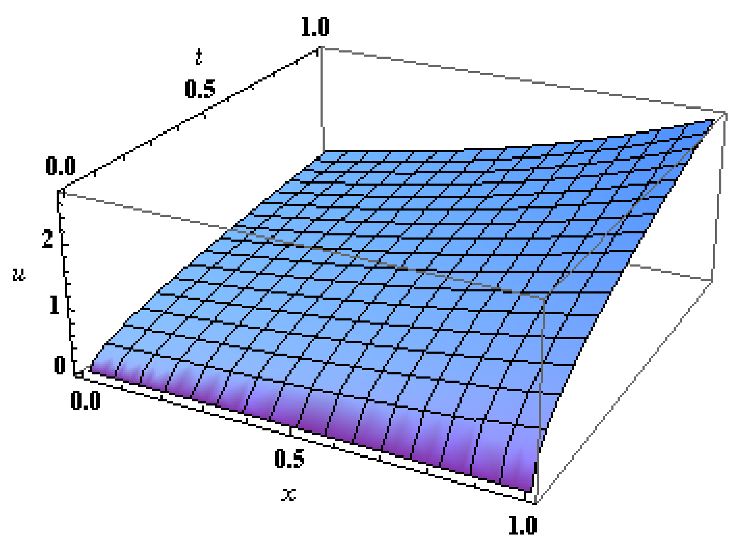
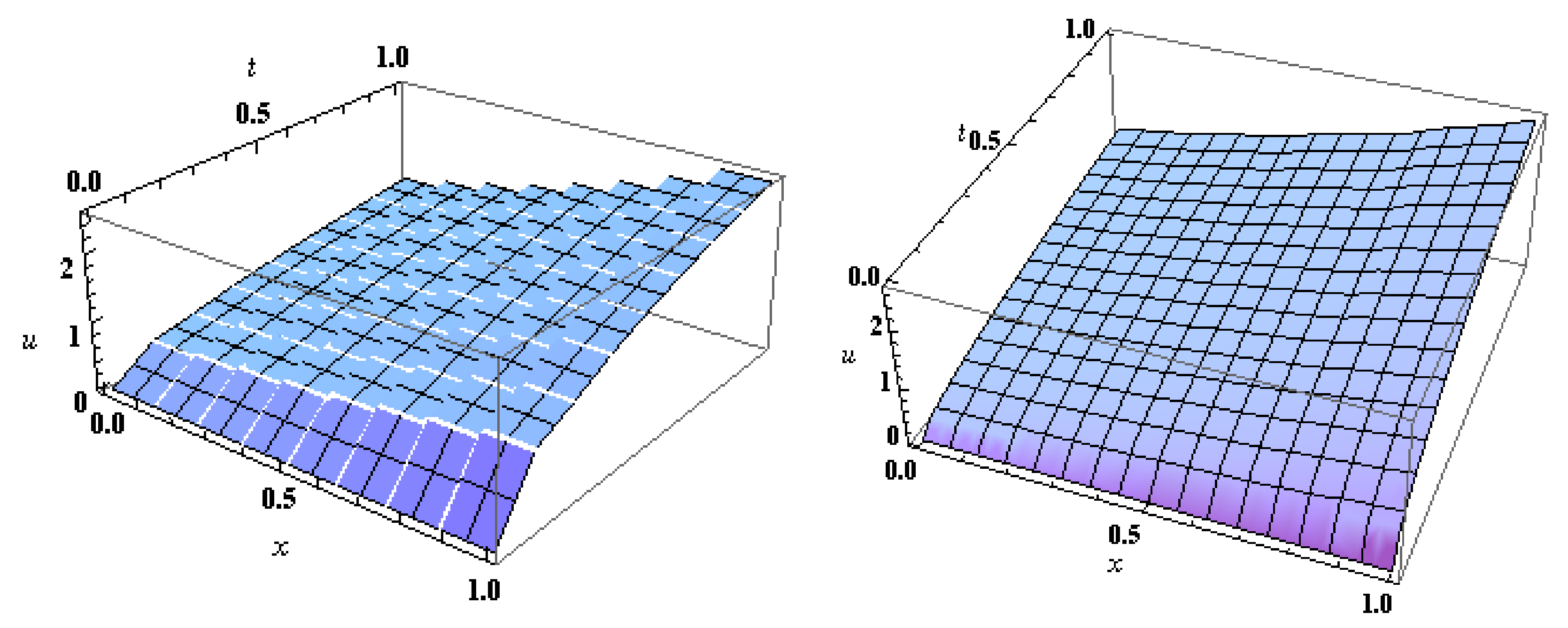
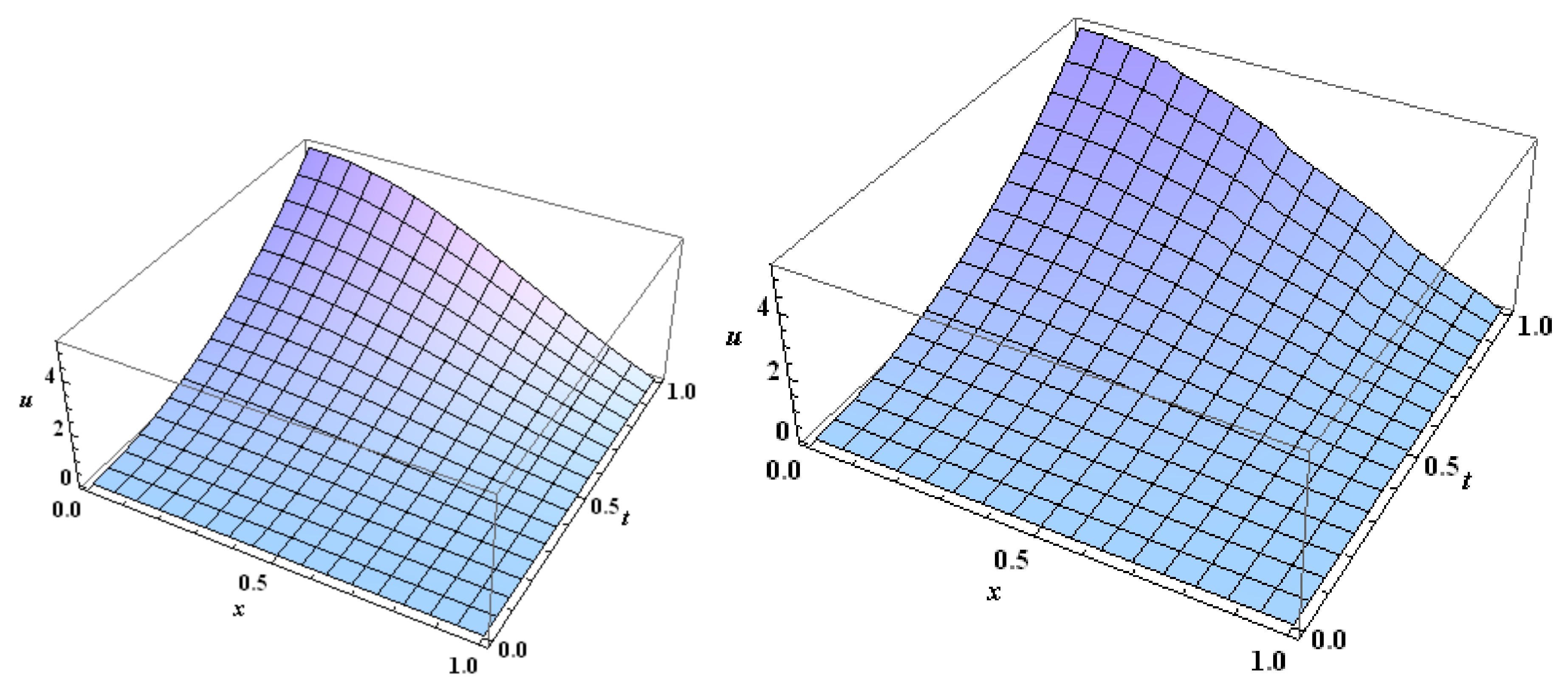
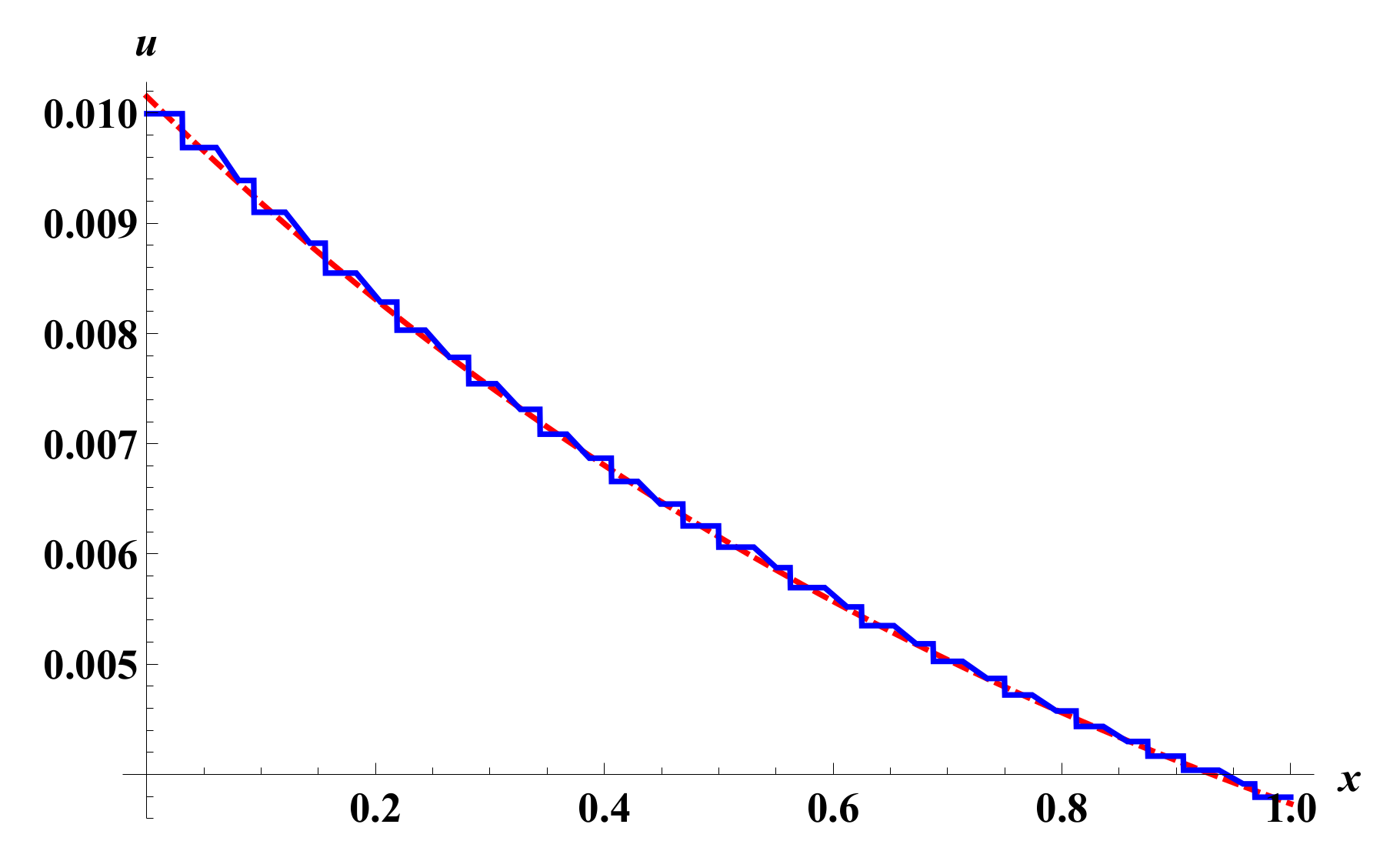
for $n,m=1,2,3,\dots ,32$, where $q_j\left(x\right):={\int }_0^x{p}_j\left(y\right)dy$. Use one of the common computer packages (we used Mathematica 11) to compute the Haar coefficients $a_{ij}$, for $n,m=1,2,3,\dots ,32.$ Figure 1, Figure 2 and Figure 3 show the exact and approximate solutions for different levels of resolution.

Second Approach:(Laplace Haar wavelet Method)

We apply the Laplace transform to Equation (11) to get

$$\sqrt{s}U(x,s)=\frac{\sqrt{\pi }}{2}\frac{1}{s}{e}^x-\frac{2(e-1)}{3s^2}+\frac{1}{s^2}{\int }_0^1{\int }_0^{1}u(y,\tau )d\tau dy$$

or, equivalently,

$$U(x,s)=\frac{\sqrt{\pi }}{2}\frac{1}{s^{3/2}}{e}^x-\frac{2(e-1)}{3s^{5/2}}+\frac{1}{s^{5/2}}{\int }_0^1{\int }_0^{1}u(y,\tau )d\tau dy$$

Now, we take the inverse Laplace transform to obtain

$$u(x,t)=\sqrt{t}{e}^x-\frac{8(e-1)}{9}\sqrt{t^3}+\frac{4\sqrt{t^3}}{3\sqrt{\pi }}{\int }_0^1{\int }_0^{1}u(y,\tau )d\tau dy.$$

To discretize the above equation, we take the nodes $x_n=t_n=\frac{n-0.5}{32}$, $n=1,2,3\dots ,32$. By this choice, we have the system

$$\sum _{n=1}^{32}\sum _{m=1}^{32}{a}_{nm}{h}_n\left(x_i\right)h_m\left(t_j\right)=\sqrt{t_j}{e}^{x_i}-\frac{8(e-1)}{9}\sqrt{t_j^3}+\frac{4\sqrt{t_j^3}}{3\sqrt{\pi }}{\int }_0^1{\int }_0^1\sum _{n=1}^{32}\sum _{m=1}^{32}{a}_{nm}{h}_n\left(y\right)h_m\left(\tau \right)d\tau dy.$$

Using the fact that ${\int }_0^1{h}_i\left(x\right)dx=p_i\left(1\right)$ for all $i=1,2,3,\dots ,32$, one can write the above system as

$$\sum _{n=1}^{32}\sum _{m=1}^{32}{a}_{nm}{h}_n\left(x_i\right)h_m\left(t_j\right)=\sqrt{t_j}{e}^{x_i}-\frac{8(e-1)}{9}\sqrt{t_j^3}+\frac{4\sqrt{t_j^3}}{3\sqrt{\pi }}\sum _{n=1}^{32}\sum _{m=1}^{32}{a}_{nm}{p}_n\left(1\right)p_m\left(1\right).$$

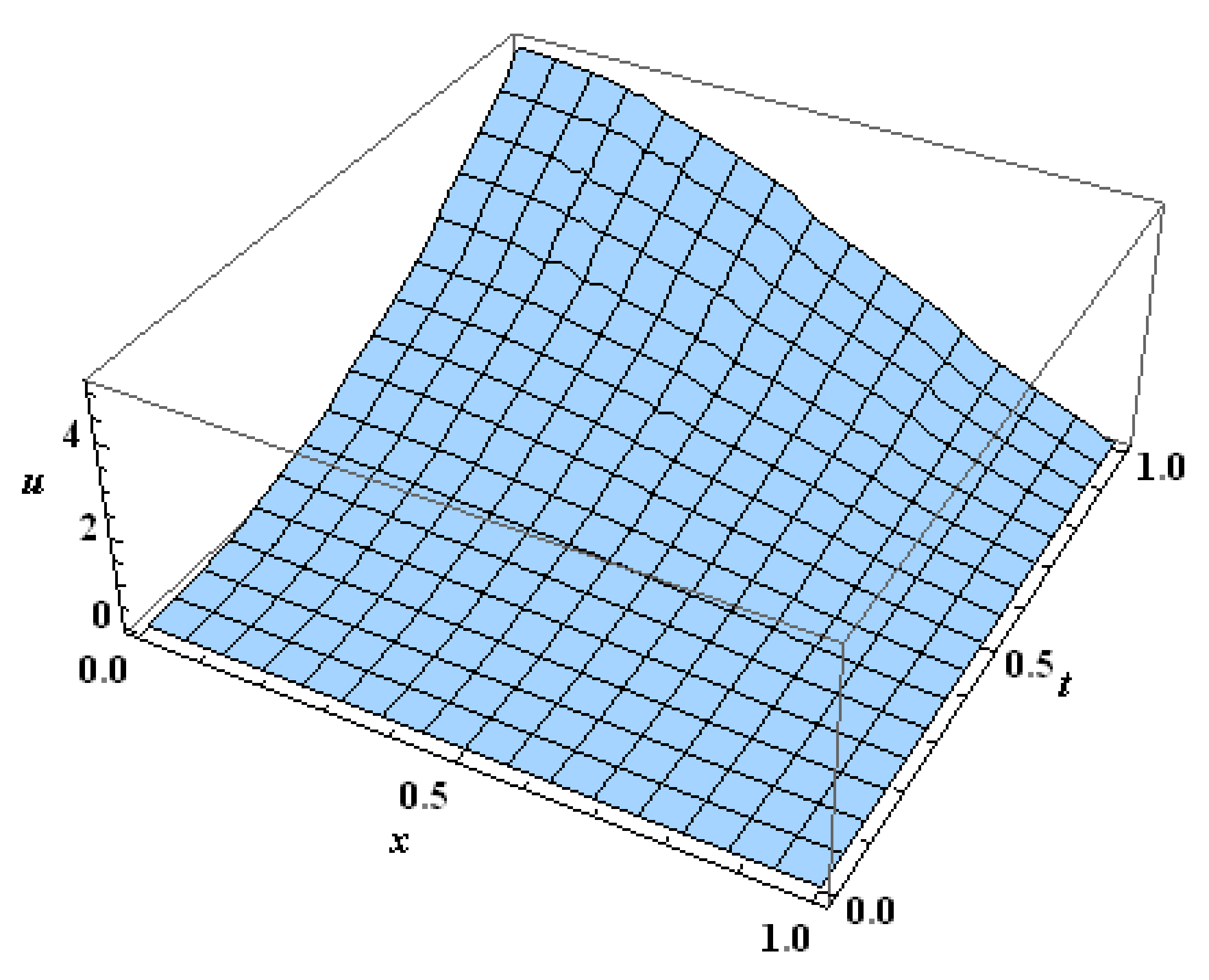
Figure 4 and Figure 5 show the graphs of the approximate solution at the level of resolution $J=4$.

Example 2.

Consider the following problem

$$D_t^{0.5}u(x,t)=6(2-e)+8t^{3/2}\mathrm{sinc}x+\pi \sqrt{\pi }{\int }_0^1{\int }_0^{1}y{e}^{\tau }u(y,\tau )dyd\tau ,$$

(14)

subject to the initial condition $u(x,0)=0$, where $\mathrm{sinc}\left(x\right)=\frac{sin\left(\pi x\right)}{\pi x}$ is the normalized sinc function. The exact solution is $u(x,t)=3\sqrt{\pi }{t}^2\mathrm{sinc}x$.

When we use the Haar wavelet method at $J=4$, we discretize Equation (14) by

$$\begin{array}{cc}\hfill \frac{1}{\sqrt{\pi }}\sum _{i=1}^{32}\sum _{j=1}^{32}{a}_{ij}{h}_i\left(x_m\right){\int }_0^{t_n}{h}_j\left(\tau \right){(t_n-\tau )}^{-0.5}d\tau & =6(2-e)+8t_n^{3/2}\mathrm{sinc}{x}_m\hfill \\ \hfill & +\pi \sqrt{\pi }\sum _{j=1}^{32}\sum _{i=1}^{32}{a}_{ij}\left({\int }_0^{1}y{h}_i\left(y\right)dy\right)\left({\int }_0^1{p}_j\left(\tau \right)e^{\tau }d\tau \right)\hfill \end{array}$$

with $x_m=\frac{m-0.5}{32}$, $t_n=\frac{n-0.5}{32}$ for $n,m=1,2,3,\dots ,32$. We solve the above system to get the approximate solution

$$u(x,t)=\sum _{j=1}^{32}\sum _{i=1}^{32}{a}_{ij}{h}_i\left(x\right)p_j\left(t\right).$$

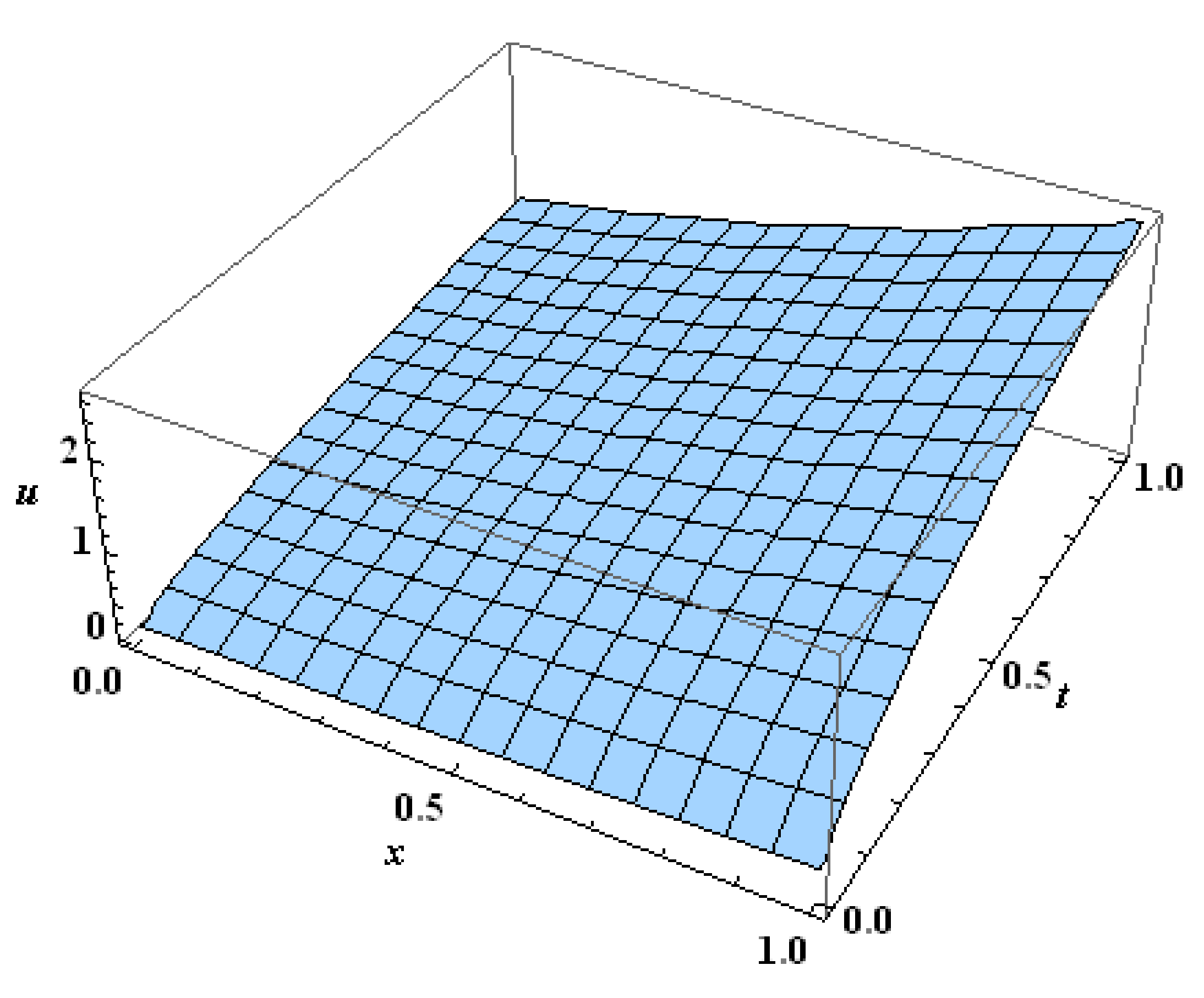
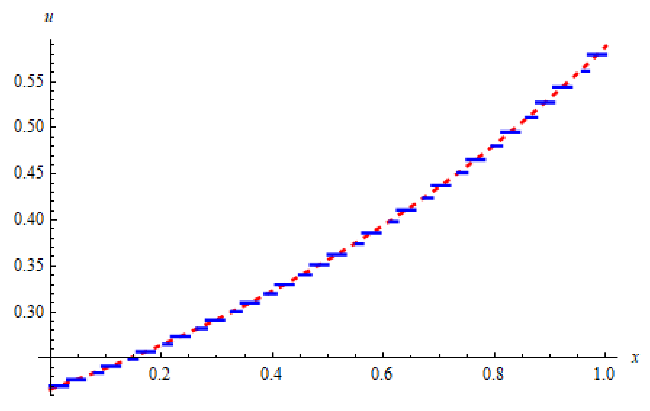
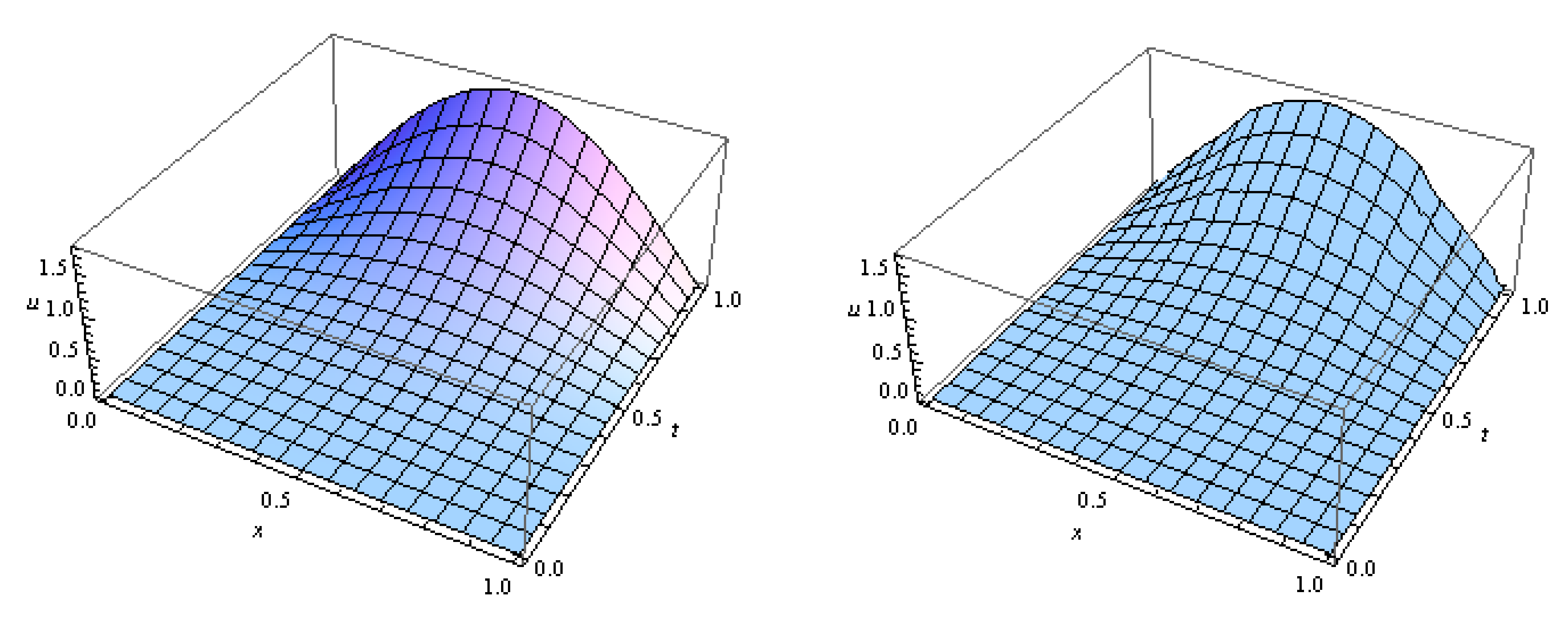
The graph of the exact solution and the approximate solution with level of resolution $J=4$ are shown in Figure 6 and Figure 7.

Now, we use the Laplace Haar wavelet method with the same level of resolution $(J=4)$. If we follow the same steps as in Example 1, we get the discrete system

$$\begin{array}{cc}\hfill \sum _{i=1}^{32}\sum _{r=1}^{32}{a}_{ir}{h}_i\left(x_m\right)h_r\left(t_n\right)& =\frac{3\sqrt{t_n}\left(8-4e+\pi \left(t_n\right){}^{3/2}\mathrm{sinc}\left(x_m\right)\right)}{\sqrt{\pi }}\hfill \\ \hfill & +2\pi \sum _{i=1}^{32}\sum _{r=1}^{32}{a}_{ir}\sqrt{t_n}\left({\int }_0^{1}x{h}_i\left(x\right)dx\right)\left({\int }_0^1{e}^t{h}_r\left(t\right)dt\right)\hfill \end{array}$$

with $x_m=\frac{m-0.5}{32}$, $t_n=\frac{n-0.5}{32}$ for $n,m=1,2,3,\dots ,32$. We solve the above system to get the approximate solution

$$u(x,t)=\sum _{j=1}^{32}\sum _{i=1}^{32}{a}_{ij}{h}_i\left(x\right)h_j\left(t\right).$$

The graph of the approximate solution with level of resolution $J=4$ is shown in Figure 8 and Figure 9.

One of the advantages of the Laplace Haar wavelet method is that one can easily solve higher order fractional integro-differential equations as explained in the methodology. The following example illustrates this benefit.

Example 3.

Consider the following third fractional order problem

$$D_t^{5/2}u(x,t)=-2{\pi }^{5/2}\left(-6+{\pi }^2\right)+12\sqrt{t}sin\left(\pi x\right){\int }_0^1{\int }_0^{1}y{e}^{\tau }u(y,\tau )dyd\tau ,$$

(15)

subject to the initial condition $u(x,0)=0.$ The exact solution is $u(x,t)=\sqrt{\pi }{t}^{3}sin\left(\pi x\right)$. We use the Laplace Haar wavelet method at the level of resolution $J=4$. The required discrete system is given by

$$\begin{array}{cc}\hfill \sum _{i=1}^{32}\sum _{r=1}^{32}{a}_{ir}{h}_i\left(x_m\right)h_r\left(t_n\right)=\frac{16}{15}{\pi }^2\left(6-{\pi }^2\right)\left(t_n\right){}^{5/2}& +\sqrt{\pi }\left(t_n\right){}^{3}sin\left(\pi x_m\right)\hfill \\ \hfill & +\frac{8{\pi }^5\sqrt{\pi }}{15}\sum _{i=1}^{32}\sum _{r=1}^{32}{a}_{ir}\left(t_n\right){}^{5/2}{p}_i\left(1\right){\int }_0^{1}sin\left(\pi t\right)h_r\left(t\right)dt,\hfill \end{array}$$

with approximate solution

$$u(x,t)=\sum _{i=1}^{32}\sum _{r=1}^{32}{a}_{ir}{h}_i\left(x_m\right)h_r\left(t_n\right).$$

Figure 10 and Figure 11 show the exact and approximate solutions for Equation (15).

5. Quadrature Laplace Haar Wavelet Method

This section is designed to apply LHWM for equations involving functions that have no closed Laplace form like $f\left(t\right)=e^{-t^2}sin\left(\sqrt{t}\right)$. We use the convolution theorem for a product of two Laplace transforms. More precisely, if $F\left(s\right)$ and $G\left(s\right)$ are the Laplace transforms for $f\left(t\right)$ and $g\left(t\right)$, respectively, then

$${\mathcal{L}}^{-1}\left[F\left(s\right)G\left(s\right)\right]\left(t\right)=f\ast g\left(t\right):={\int }_0^{t}f(t-\tau )g\left(\tau \right)d\tau .$$

Consider the same equation

$$D_t^{\alpha }u(x,t)=f(x,t)+{\int }_0^1{\int }_0^{1}k(x,t,y,\tau )u(y,\tau )dyd\tau$$

(16)

for $n-1<\alpha <n$ and initial conditions

$$u(x,0)=\frac{\partial }{\partial t}u(x,0)=\dots =\frac{{\partial }^{n-1}}{\partial t^{n-1}}u(x,0)=0.$$

(17)

Definition 4.

For $\alpha >0$, we define $\mathcal{G}\left(t\right)=\frac{t^{\alpha -1}}{\mathsf{\Gamma }\left(\alpha \right)}$ for $0<t<\infty$.

Notice that $\mathcal{L}\left[\mathcal{G}\left(t\right)\right]\left(s\right)=\frac{1}{s^{\alpha }}$. This fact will be the key of this section. Take the Laplace transform for both sides of Equation (16), and keep in your mind the initial conditions (17), one obtains

$$U(x,s)=\frac{1}{s^{\alpha }}F(x,s)+{\int }_0^1{\int }_0^1\frac{1}{s^{\alpha }}K(x,s,y,\tau )u(y,\tau )dyd\tau$$

(18)

Now, take the inverse Laplace transform for both sides of Equation (18) and use the convolution theorem, to find that

$$u(x,s)=\mathcal{G}\ast f(x,t)+{\int }_0^1{\int }_0^1\mathcal{G}\ast k(x,t,y,\tau )u(y,\tau )dyd\tau ,$$

(19)

where

$$\mathcal{G}\ast f(x,t)={\int }_0^t\mathcal{G}(t-w)f(x,w)dw$$

and

$$\mathcal{G}\ast k(x,t,y,\tau )={\int }_0^t\mathcal{G}(t-w)k(x,w,y,\tau )dw$$

If we use any of the quadrature formulas to estimate these integrals, we obtain the new Fredholm integral equation

$$u(x,s)=\tilde{f}(x,t)+{\int }_0^1{\int }_0^1\tilde{k}(x,t,y,\tau )u(y,\tau )dyd\tau ,$$

(20)

where

$$\tilde{f}(x,t)=\frac{t}{M}\sum _{j=1}^M\mathcal{G}(t-w_j)f(x,w_j)$$

and

$$\tilde{k}(x,t,y,\tau )=\frac{t}{M}\sum _{j=1}^M\mathcal{G}(t-w_j)k(x,w_j,y,\tau )$$

for $w_j=\frac{t}{M}j$. We emphasize that one can take any quadrature formula to estimate the above convolutions. Finally, we discretize Equation (20), for desired resolution J as before, to get the approximate solution

$$u(x,t)\approx \sum _{i=1}^{2^{J+1}}\sum _{j=1}^{2^{J+1}}{a}_{ij}{h}_i\left(x\right)h_j\left(t\right).$$

Example 4.

Consider the following higher order fractional integro-differential equation

$$D_t^{3/2}u(x,t)=\frac{3}{4}{e}^{-x}\sqrt{\pi }+\frac{4}{5}{e}^{-t^2}sin\sqrt{t}+{\int }_0^1{\int }_0^1\frac{2e^{1-t^2}}{1-e}sin\sqrt{t}u(y,\tau )dyd\tau ,$$

(21)

subject to the initial conditions $u(x,0)=\frac{\partial }{\partial t}u(x,0)=0.$ The exact solution is $u(x,t)=e^{-x}{t}^{3/2}$. We use the Laplace Haar wavelet method at the level of resolution $J=4$. The required discrete system is given by

$$\begin{array}{cc}\hfill \sum _{i=1}^{32}\sum _{r=1}^{32}{a}_{ir}{h}_i\left(x_m\right)h_r\left(t_n\right)=\tilde{f}(x_m,t_n)+& \sum _{i=1}^{32}\sum _{r=1}^{32}{a}_{ir}{\int }_0^1{\int }_0^1\tilde{k}(x_m,t_n,y,\tau )h_i\left(y\right)h_r\left(\tau \right)dyd\tau ,\hfill \end{array}$$

with approximate solution

$$u(x,t)=\sum _{i=1}^{32}\sum _{r=1}^{32}{a}_{ir}{h}_i\left(x_m\right)h_r\left(t_n\right).$$

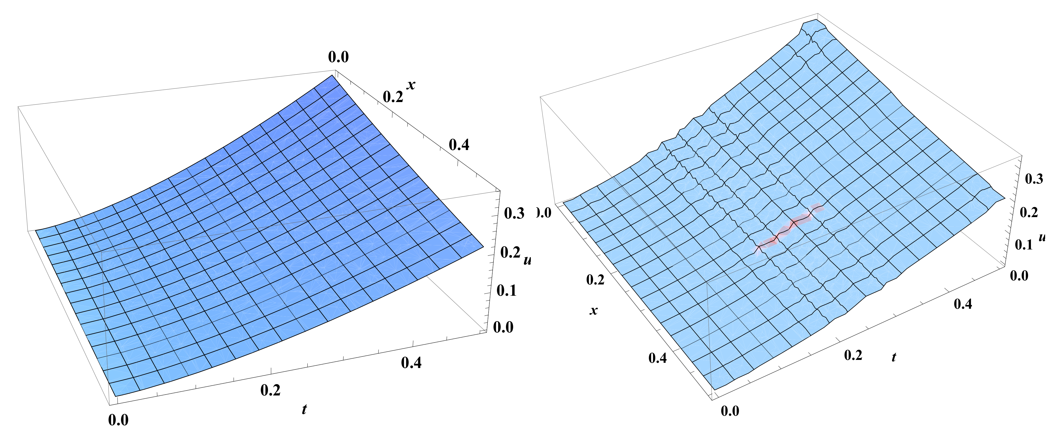
Figure 12 and Figure 13 show the exact and approximate solutions for Equation (21).

6. Comparison between HWM and LHWM

In this section, we compare the Haar wavelet method and Laplace Haar wavelet method. The

Table 2. Exact, approximate, and absolute error for different values of $x_m$ and $t_n$ in Example 1 with resolution $J=4$ using HWM.

${\mathit{x}}_{\mathit{m}}$	${\mathit{t}}_{\mathit{n}}$	Exact Value	Approximate Value	Absolute Error
0.015625		0.126968	0.0997192	2.72493$\times$10${}^{-}$${}^2$
0.109375		0.139448	0.10952	2.99273$\times$10${}^{-}$${}^2$
0.234375	0.015625	0.158015	0.124103	3.39119$\times$10${}^{-}$${}^2$
0.484375		0.202895	0.159352	4.35433$\times$10${}^{-}$${}^2$
0.734375		0.260522	0.202896	5.59102$\times$10${}^{-}$${}^2$
0.984375		0.334517	0.262728	7.17897$\times$10${}^{-}$${}^2$
0.015625		0.335927	0.336167	2.39687$\times$10${}^{-}$${}^4$
0.109375		0.368944	0.369209	2.65744$\times$10${}^{-}$${}^4$
0.234375	0.109375	0.418068	0.418372	3.04514$\times$10${}^{-}$${}^4$
0.484375		0.53681	0.537208	3.98226$\times$10${}^{-}$${}^4$
0.734375		0.689277	0.689796	5.18554$\times$10${}^{-}$${}^4$
0.984375		0.88505	0.885723	6.73059$\times$10${}^{-}$${}^4$
0.015625		0.491747	0.49167	7.68371$\times$10${}^{-5}$
0.109375		0.540078	0.540002	7.65043$\times$10${}^{-5}$
0.234375	0.234375	0.611989	0.611913	7.60092$\times$10${}^{-5}$
0.484375		0.785809	0.785734	7.48123$\times$10${}^{-5}$
0.734375		1.009	1.00893	7.32756$\times$10${}^{-5}$
0.984375		1.29558	1.29551	7.13023$\times$10${}^{-5}$
0.015625		0.70693	0.706692	2.38435$\times$10${}^{-4}$
0.109375		0.776411	0.776173	2.38395$\times$10${}^{-4}$
0.234375	0.484375	0.879789	0.879551	2.38335$\times$10${}^{-4}$
0.484375		1.12967	1.12943	2.38189$\times$10${}^{-4}$
0.734375		1.45053	1.45029	2.38002$\times$10${}^{-4}$
0.984375		1.86251	1.86228	2.37762$\times$10${}^{-4}$
0.015625		1.00778	1.00709	6.92453$\times$10${}^{-4}$
0.109375		1.10683	1.10614	6.92446$\times$10${}^{-4}$
0.234375	0.984375	1.2542	1.25351	6.92437$\times$10${}^{-4}$
0.484375		1.61043	1.60974	6.92415$\times$10${}^{-4}$
0.734375		2.06783	2.06714	6.92386$\times$10${}^{-4}$
0.984375		2.65515	2.65446	6.92349$\times$10${}^{-4}$

,

Table 3. Exact, approximate, and absolute error for different values of $x_m$ and $t_n$ in Example 1 with resolution $J=4$ using LHWM.

${\mathit{x}}_{\mathit{m}}$	${\mathit{t}}_{\mathit{n}}$	Exact Value	Approximate Value	Absolute Error
0.015625		0.126968	0.12697	1.04314$\times$10${}^{-6}$
0.109375		0.139448	0.139449	1.04314$\times$10${}^{-6}$
0.234375	0.015625	0.158015	0.158016	1.04314$\times$10${}^{-6}$
0.484375		0.202895	0.202896	1.04314$\times$10${}^{-6}$
0.734375		0.260522	0.260523	1.04314$\times$10${}^{-6}$
0.984375		0.334517	0.334518	1.04314$\times$10${}^{-6}$
0.015625		0.335927	0.335946	1.93192$\times$10${}^{-5}$
0.109375		0.368944	0.368963	1.93192$\times$10${}^{-5}$
0.234375	0.109375	0.418068	0.418087	1.93192$\times$10${}^{-5}$
0.484375		0.53681	0.536829	1.93192$\times$10${}^{-5}$
0.734375		0.689277	0.689297	1.93192$\times$10${}^{-5}$
0.984375		0.88505	0.885069	1.93192$\times$10${}^{-5}$
0.015625		0.491747	0.491807	6.06008$\times$10${}^{-5}$
0.109375		0.540078	0.540139	6.06008$\times$10${}^{-5}$
0.234375	0.234375	0.611989	0.612049	6.06008$\times$10${}^{-5}$
0.484375		0.785809	0.78587	6.06008$\times$10${}^{-5}$
0.734375		1.009	1.00906	6.06008$\times$10${}^{-5}$
0.984375		1.29558	1.29564	6.06008$\times$10${}^{-5}$
0.015625		0.70693	0.707111	1.80046$\times$10${}^{-4}$
0.109375		0.776411	0.776591	1.80046$\times$10${}^{-4}$
0.234375	0.484375	0.879789	0.879969	1.80046$\times$10${}^{-4}$
0.484375		1.12967	1.12985	1.80046$\times$10${}^{-4}$
0.734375		1.45053	1.45071	1.80046$\times$10${}^{-4}$
0.984375		1.86251	1.86269	1.80046$\times$10${}^{-4}$
0.015625		1.00778	1.0083	5.21618$\times$10${}^{-4}$
0.109375		1.10683	1.10735	5.21618$\times$10${}^{-4}$
0.234375	0.984375	1.2542	1.25473	5.21618$\times$10${}^{-4}$
0.484375		1.61043	1.61095	5.21618$\times$10${}^{-4}$
0.734375		2.06783	2.06835	5.21618$\times$10${}^{-4}$
0.984375		2.65515	2.65567	5.21618$\times$10${}^{-4}$

,

Table 4. Exact, approximate, and absolute error for different values of $x_m$ and $t_n$ in Example 2 with resolution $J=4$ using HWM.

${\mathit{x}}_{\mathit{m}}$	${\mathit{t}}_{\mathit{n}}$	Exact Value	Approximate Value	Absolute Error
0.015625		0.00129766	0.00190396	6.06298$\times$10${}^{-}$${}^4$
0.109375		0.00127279	0.00187079	5.98006$\times$10${}^{-}$${}^4$
0.234375		0.00118402	0.00175244	5.68417$\times$10${}^{-}$${}^4$
0.359375	0.015625	0.00103945	0.00155967	5.20225$\times$10${}^{-}$${}^4$
0.484375		0.000852082	0.00130985	4.57771$\times$10${}^{-}$${}^4$
0.734375		0.000416925	0.000729643	3.12718$\times$10${}^{-}$${}^4$
0.984375		0.0000205978	0.000201207	1.80609$\times$10${}^{-}$${}^4$
0.015625		0.0635855	0.0631889	3.96607$\times$10${}^{-}$${}^4$
0.109375		0.0623666	0.0619889	3.77777$\times$10${}^{-}$${}^4$
0.234375		0.058017	0.0577064	3.10578$\times$10${}^{-}$${}^4$
0.359375	0.109375	0.0509328	0.0507317	2.01132$\times$10${}^{-}$${}^4$
0.484375		0.041752	0.0416927	5.92945$\times$10${}^{-}$${}^4$
0.734375		0.0204293	0.0206995	2.70127$\times$10${}^{-}$${}^4$
0.984375		0.00100929	0.00157945	5.70154$\times$10${}^{-}$${}^4$
0.015625		0.291974	0.291125	8.49444$\times$10${}^{-}$${}^4$
0.109375		0.286377	0.285561	8.16738$\times$10${}^{-}$${}^4$
0.234375		0.266405	0.265705	7.00023$\times$10${}^{-}$${}^4$
0.359375	0.234375	0.233875	0.233365	5.0993$\times$10${}^{-}$${}^4$
0.484375		0.191718	0.191455	2.63576$\times$10${}^{-}$${}^4$
0.734375		0.0938081	0.0941167	3.08585$\times$10${}^{-}$${}^4$
0.984375		0.00463451	0.0054642	8.29692$\times$10${}^{-}$${}^4$
0.015625		1.24705	1.2456	1.45855$\times$10${}^{-}$${}^3$
0.109375		1.22315	1.22174	1.40698$\times$10${}^{-}$${}^3$
0.234375		1.13784	1.13662	1.22295$\times$10${}^{-}$${}^3$
0.359375	0.484375	0.998907	0.997984	9.23228$\times$10${}^{-4}$
0.484375		0.81885	0.818316	5.34797$\times$10${}^{-4}$
0.734375		0.400665	0.401032	3.67342$\times$10${}^{-4}$
0.984375		0.0197945	0.0209835	1.18898$\times$10${}^{-}$${}^3$
0.015625		5.15042	5.14813	2.29639$\times$10${}^{-}$${}^3$
0.109375		5.0517	5.04948	2.21871$\times$10${}^{-}$${}^3$
0.234375		4.69938	4.69744	1.94151$\times$10${}^{-}$${}^3$
0.359375	0.984375	4.12556	4.12407	1.49005$\times$10${}^{-}$${}^3$
0.484375		3.38191	3.38101	9.04961$\times$10${}^{-}$${}^4$
0.734375		1.65478	1.65523	4.53913$\times$10${}^{-}$${}^4$
0.984375		0.0817527	0.0834443	1.69153$\times$10${}^{-}$${}^3$

,

Table 5. Exact, approximate, and absolute error for different values of $x_m$ and $t_n$ in Example 2 with resolution $J=4$ using LHWM.

${\mathit{x}}_{\mathit{m}}$	${\mathit{t}}_{\mathit{n}}$	Exact Value	Approximate Value	Absolute Error
0.015625		0.00129766	0.00130173	4.06726$\times$10${}^{-6}$
0.109375		0.00127279	0.00127686	4.06726$\times$10${}^{-6}$
0.234375		0.00118402	0.00118809	4.06726$\times$10${}^{-6}$
0.359375	0.015625	0.00103945	0.00104351	4.06726$\times$10${}^{-6}$
0.484375		0.000852082	0.000856149	4.06726$\times$10${}^{-6}$
0.734375		0.000416925	0.000420992	4.06726$\times$10${}^{-6}$
0.984375		0.0000205978	0.000246651	4.06726$\times$10${}^{-6}$
0.015625		0.0635855	0.0635962	1.0761$\times$10${}^{-5}$
0.109375		0.0623666	0.0623774	1.0761$\times$10${}^{-5}$
0.234375		0.058017	0.0580278	1.0761$\times$10${}^{-5}$
0.359375	0.109375	0.0509328	0.0509436	1.0761$\times$10${}^{-5}$
0.484375		0.041752	0.0417628	1.0761$\times$10${}^{-5}$
0.734375		0.0204293	0.0204401	1.0761$\times$10${}^{-5}$
0.984375		0.00100929	0.00102005	1.0761$\times$10${}^{-5}$
0.015625		0.291974	0.29199	1.57524$\times$10${}^{-5}$
0.109375		0.286377	0.286393	1.57524$\times$10${}^{-5}$
0.234375		0.266405	0.26642	1.57524$\times$10${}^{-5}$
0.359375	0.234375	0.233875	0.233891	1.57524$\times$10${}^{-5}$
0.484375		0.191718	0.191734	1.57524$\times$10${}^{-5}$
0.734375		0.0938081	0.0938239	1.57524$\times$10${}^{-5}$
0.984375		0.00463451	0.00465026	1.57524$\times$10${}^{-5}$
0.015625		1.24705	1.24708	2.26455$\times$10${}^{-5}$
0.109375		1.22315	1.22317	2.26455$\times$10${}^{-5}$
0.234375		1.13784	1.13787	2.26455$\times$10${}^{-5}$
0.359375	0.484375	0.998907	0.99893	2.26455$\times$10${}^{-5}$
0.484375		0.81885	0.818873	2.26455$\times$10${}^{-5}$
0.734375		0.400665	0.400688	2.26455$\times$10${}^{-5}$
0.984375		0.0197945	0.0198172	2.26455$\times$10${}^{-5}$
0.015625		5.15042	5.15046	3.22829$\times$10${}^{-5}$
0.109375		5.0517	5.05173	3.22829$\times$10${}^{-5}$
0.234375		4.69938	4.69941	3.22829$\times$10${}^{-5}$
0.359375	0.984375	4.12556	4.12559	3.22829$\times$10${}^{-5}$
0.484375		3.38191	3.38194	3.22829$\times$10${}^{-5}$
0.734375		1.65478	1.65481	3.22829$\times$10${}^{-5}$
0.984375		0.0817527	0.081785	3.22829$\times$10${}^{-5}$

and

Table 6. Exact, approximate, and absolute error for different values of $x_m$ and $t_n$ in Example 3 with resolution $J=4$ using HWM.

${\mathit{x}}_{\mathit{m}}$	${\mathit{t}}_{\mathit{n}}$	Exact Value	Approximate Value	Absolute Error
0.015625		3.31765$\times$10${}^{-7}$	3.02178$\times$10${}^{-7}$	2.95868$\times$10${}^{-8}$
0.046875		9.921$\times$10${}^{-7}$	9.62513$\times$10${}^{-7}$	2.95868$\times$10${}^{-8}$
0.109375		2.27784$\times$10${}^{-6}$	2.24825$\times$10${}^{-6}$	2.95868$\times$10${}^{-8}$
0.234375	0.015625	4.54066$\times$10${}^{-6}$	4.51108$\times$10${}^{-6}$	2.95868$\times$10${}^{-8}$
0.359375		6.11221$\times$10${}^{-6}$	6.08262$\times$10${}^{-6}$	2.95868$\times$10${}^{-8}$
0.484375		6.75323$\times$10${}^{-6}$	6.72364$\times$10${}^{-6}$	2.95868$\times$10${}^{-8}$
0.734375		5.00985$\times$10${}^{-6}$	4.98026$\times$10${}^{-6}$	2.95868$\times$10${}^{-8}$
0.984375		3.31765$\times$10${}^{-7}$	3.02178$\times$10${}^{-7}$	2.95868$\times$10${}^{-8}$
0.015625		0.000113795	0.00010996	3.83569$\times$10${}^{-6}$
0.046875		0.00034029	0.000336455	3.83569$\times$10${}^{-6}$
0.109375		0.000781299	0.000777463	3.83569$\times$10${}^{-6}$
0.234375	0.109375	0.00155745	0.00155361	3.83569$\times$10${}^{-6}$
0.359375		0.00209649	0.00209265	3.83569$\times$10${}^{-6}$
0.484375		0.00231636	0.00231252	3.83569$\times$10${}^{-6}$
0.734375		0.00171838	0.00171454	3.83569$\times$10${}^{-6}$
0.984375		0.000113795	0.00010996	3.83569$\times$10${}^{-6}$
0.015625		0.00111971	0.00109392	2.57826$\times$10${}^{-5}$
0.046875		0.00334834	0.00332255	2.57826$\times$10${}^{-5}$
0.109375		0.00768771	0.00766192	2.57826$\times$10${}^{-5}$
0.234375	0.234375	0.0153247	0.015299	2.57826$\times$10${}^{-5}$
0.359375		0.0206287	0.0206029	2.57826$\times$10${}^{-5}$
0.484375		0.0227922	0.0227664	2.57826$\times$10${}^{-5}$
0.734375		0.0169082	0.0168825	2.57826$\times$10${}^{-5}$
0.984375		0.00111971	0.00109392	2.57826$\times$10${}^{-5}$
0.015625		0.00988361	0.0097253	1.58308$\times$10${}^{-4}$
0.046875		0.0295556	0.0293973	1.58308$\times$10${}^{-4}$
0.109375		0.0678591	0.0677008	1.58308$\times$10${}^{-4}$
0.234375	0.484375	0.135271	0.135113	1.58308$\times$10${}^{-4}$
0.359375		0.182089	0.181931	1.58308$\times$10${}^{-4}$
0.484375		0.201185	0.201027	1.58308$\times$10${}^{-4}$
0.734375		0.149248	0.14909	1.58308$\times$10${}^{-4}$
0.984375		0.00988361	0.0097253	1.58308$\times$10${}^{-4}$
0.015625		0.0829568	0.0820248	9.32073$\times$10${}^{-4}$
0.046875		0.248072	0.247139	9.32073$\times$10${}^{-4}$
0.109375		0.569567	0.568635	9.32073$\times$10${}^{-4}$
0.234375	0.984375	1.13538	1.13445	9.32073$\times$10${}^{-4}$
0.359375		1.52834	1.52741	9.32073$\times$10${}^{-4}$
0.484375		1.68863	1.68769	9.32073$\times$10${}^{-4}$
0.734375		1.2527	1.25177	9.32073$\times$10${}^{-4}$
0.984375		0.0829568	0.0820248	9.32073$\times$10${}^{-4}$

below show the absolute error in Examples 1–3 in both methods. The tables indicate the accuracy of both methods, whereas the Laplace Haar wavelet method has better approximation. It is worth mentioning that the Laplace wavelet method reduces the computation times significantly (see

Table 7. Comparison between HWM and LHWM.

	Example(1) Using HWM	Example(1) Using LHWM	Example(2) Using HWM	Example(2) Using LHWM
Computations time using Mathematica 11, at J = 2	24 min	3 min	28 min	3.5 min
Computations time using Mathematica 11, at J = 4	3 h and 20 min	10 min	4 h and 35 min	12 min
Erorr range at J = 4	10${}^{-4}$–10${}^{-2}$	10${}^{-6}$–10${}^{-4}$	10${}^{-4}$–10${}^{-3}$	10${}^{-6}$–10${}^{-5}$

).

7. Conclusions

We started our own work by applying the existing method, Haar wavelet method, to solve two-dimensional fractional integro-differential equations. However, we aspire to get better results in less time. As a result, we proposed the Laplace Haar wavelet method to solve these kinds of equations. Applying the Laplace Haar wavelet method was beneficial. It reduced the error and the computational time significantly.

In conclusion, applying the Laplace Haar wavelet method is advantageous in comparison with the Haar wavelet method.

References

1. Heil, C.E.; Walnut, D.F. Continuous and discrete wavelet transforms. SIAM Rev. 1989, 31, 628–666. [Google Scholar] [CrossRef] [Green Version]
2. Daubechies, I. Ten Lectures on Wavelets; SIAM: Philadelphia, PA, USA, 1992; Volume 61. [Google Scholar]
3. Kyed, M. Square Integrable Representations and the Continuous Wavelet Transformation. Ph.D. Thesis, Aarhus University, Aarhus, Denmark, 1999. [Google Scholar]
4. Babolian, E.; Shahsavaran, A. Numerical solution of nonlinear Fredholm integral equations of the second kind using Haar wavelets. J. Comput. Appl. Math. 2009, 225, 87–95. [Google Scholar] [CrossRef] [Green Version]
5. Lepik, Ü. Solving fractional integral equations by the Haar wavelet method. Appl. Math. Comput. 2009, 214, 468–478. [Google Scholar] [CrossRef]
6. Aziz, I.; Fayyaz, M. A new approach for numerical solution of integro-differential equations via Haar wavelets. Int. J. Comput. Math. 2013, 90, 1971–1989. [Google Scholar]
7. Aziz, I. New algorithms for the numerical solution of nonlinear Fredholm and Volterra integral equations using Haar wavelets. J. Comput. Appl. Math. 2013, 239, 333–345. [Google Scholar] [CrossRef]
8. Ur Rehman, M.; Khan, R.A. The Legendre wavelet method for solving fractional differential equations. Commun. Nonlinear Sci. Numer. Simul. 2011, 16, 4163–4173. [Google Scholar] [CrossRef]
9. Pedas, A.; Tamme, E. Spline collocation methods for linear multi-term fractional differential equations. J. Comput. Appl. Math. 2011, 236, 167–176. [Google Scholar] [CrossRef] [Green Version]
10. Cattani, C. Shannon wavelets for the solution of integrodifferential equations. Math. Probl. Eng. 2010, 2010. [Google Scholar] [CrossRef] [Green Version]
11. Diethelm, K.; Ford, N.J. Analysis of fractional differential equations. J. Math. Anal. Appl. 2002, 265, 229–248. [Google Scholar] [CrossRef] [Green Version]
12. Boggess, A.; Narcowich, F.J. A First, Course in Wavelets with Fourier Analysis; John Wiley & Sons: Hoboken, NJ, USA, 2015. [Google Scholar]
13. Ishteva, M.; Boyadjiev, L.; Scherer, R. On the Caputo operator of fractional calculus and C-Laguerre functions. Math. Sci. Res. J. 2005, 9, 161. [Google Scholar]
14. Richard, H. Fractional Calculus: An Introduction for Physicists; World Scientific: Singapore, 2014. [Google Scholar]
15. Caputo, M. Linear models of dissipation whose Q is almost frequency independent—II. Geophys. J. Int. 1967, 13, 529–539. [Google Scholar] [CrossRef]
16. Kexue, L.; Jigen, P. Laplace transform and fractional differential equations. Appl. Math. Lett. 2011, 24, 2019–2023. [Google Scholar] [CrossRef] [Green Version]
Figure 1. The exact solution for Example 1.
Algorithms 13 00037 g001
Figure 2. The approximate solution for Example 1 at J = 2 (to the left) and at J = 4 (to the right) using HWM.
Algorithms 13 00037 g002
Figure 3. The approximate solution (blue) and the exact solution (red) for Example 1 at J = 2 , t = 0.046875 (to the left) and at J = 4 , t = 0.046875 (to the right) using HWM.
Algorithms 13 00037 g003
Figure 4. The approximate solution for Example 1 with level of resolution J = 4 using LHWM.
Algorithms 13 00037 g004
Figure 5. The approximate solution (blue) and the exact solution (red) for Example 1 with level of resolution J = 4 and t = 0.5 using LHWM.
Algorithms 13 00037 g005
Figure 6. The exact solution (to the left) and the approximate solution (to the right) at J = 4 for Example 2.
Algorithms 13 00037 g006
Figure 7. The approximate solution (blue) and the exact solution (red) for Example 2 with level of resolution J = 4 and t = t 8 using HWM.
Algorithms 13 00037 g007
Figure 8. The approximate solution for Example 2 with level of resolution J = 4 using LHWM.
Algorithms 13 00037 g008
Figure 9. The approximate solution (blue) and the exact solution (red) for Example 2 with level of resolution J = 4 and t = t 8 using LHWM.
Algorithms 13 00037 g009
Figure 10. The exact (to the left) and the approximate (to the right) solutions for Example 3 with J = 4 using LHWM.
Algorithms 13 00037 g010
Figure 11. The approximate solution (blue) and the exact solution (red) for Example 3 with level of resolution J = 4 and t = t 8 using LHWM.
Algorithms 13 00037 g011
Figure 12. The exact (to the left) and the approximate (to the right) solutions for Example 4 with J = 4 using LHWM.
Algorithms 13 00037 g012
Figure 13. The approximate solution (blue) and the exact solution (red) for Example 4 with level of resolution J = 4 and t = t 2 using LHWM.
Algorithms 13 00037 g013