1. Introduction
For the last two decades, an important effort has been made to propose and analyze new mathematical epidemic models being based on integro-differential equations and/or difference equations. Such models are claimed to describe the evolution through time of the various subpopulations integrated in the epidemic model under study whose respective dynamics are coupled. A classical, so-called, SEIR (susceptible-exposed-infectious-recovered) epidemic model splits the total infectious population into two subpopulations (or compartments), namely, the so-called “infected” or “exposed” (E) (those having the disease but do not present yet external symptoms) and the “Infectious” or “Infective” (I) (those having external symptoms). The mentioned basic SEIR model has nowadays multiple variants with different degrees of complexity. See, for instance, [
1,
2,
3,
4,
5,
6,
7,
8,
9,
10,
11,
12,
13,
14] and some of the references therein. In particular, one can refer to those ones which admit controls like constant and feedback vaccination and treatment controls and/or impulsive controls (exerted on very short periods of time) or those involving several interacting patches associated to different towns ort regions. For instance, an optimization approach is given to get the vaccination controls in [
7]. In [
9,
10,
11], some pulse vaccination strategies are proposed. In [
11,
12] several strategies are discussed including feedback. In [
13], an epidemic model is proposed which is subject to a ratio-dependent saturation incidence rate. On the other hand, a SIR (susceptible-infectious-recovered) epidemic model under impulsive vaccination was investigated in [
14] while a non- autonomous SIRVS epidemic model subject to vaccination controls has been proposed and discussed in [
15]. Also, an epidemic delayed model with diffusion has been characterized in [
16]. It has to be mentioned that a relevant attention has been paid to the investigation of the stability and positivity properties of epidemic models in both the vaccination-free and vaccination control situations. See, for instance, [
17,
18,
19,
20,
21,
22,
23,
24,
25,
26,
27,
28,
29]. The positivity properties of de solutions and equilibrium points of some epidemic models are studied in detail in [
30,
31,
32,
33], while model discretization concerns are discussed in [
33,
34] and relationships to thermodynamics concepts are discussed in [
35]. On the other hand, epidemics evolution and concerns regarding COVID-19 are being described in more recent works. See, for instance, [
36,
37,
38,
39,
40,
41,
42,
43,
44,
45,
46,
47,
48,
49,
50,
51,
52,
53,
54,
55,
56,
57] and references in their model. It can be pointed out that the approaches of [
19,
20] and [
58] are formulated in the stochastic framework context. In particular, the epidemic model proposed in [
58] can be interpreted as an interpolation between a SI model and an SIR model.
On the other hand, it is well- known that there may be some individuals who are infective so that they can produce contagions to susceptible individuals but do not have significant external symptoms. Those ones are the members of the so-called “Asymptomatic” (A) subpopulation, [
4,
31,
32,
33]. This subpopulation appears even in the common known influenza disease. If such an asymptomatic subpopulation is incorporated to the model, then it turns out that the exposed might have distinct transitions to the symptomatic infectious and to the asymptomatic ones. In this way, a proportion of the exposed become asymptomatic after a certain time period while another proportion becomes infectious after a certain period of time. In general, both respective proportions might be distinct. In the Ebola disease, the lying dead corpses are also infective [
4,
5,
6,
31,
32,
33] which can cause very serious sanitary problems in third world tropical countries with low or scarce sanitary means. In particular, SEIADR-type models are considered in [
31,
32,
33] which incorporate asymptomatic and dead populations to the typical SEIR models, and which include, in general, vaccination and treatment controls as well as impulsive controls to retire the infective bodies from the streets in third world countries hit by Ebola outbreaks.
This paper proposes and investigates an extended SEIR epidemic model with seven subpopulations, namely, the so-called SE(Is)(Ih)(Icicu)AR epidemic model, under the points of view of fulfilling general suitable properties like, for instance, the positivity and stability of the solutions and its output controllability properties for appropriately defined outputs which fix the maximum levels of reasonable presence of hospitalized patients at certain checking time instants. The model contains as integrated subpopulations the susceptible (S) and the recovered (R) subpopulations plus five more infective subpopulations which are the Exposed subpopulation (
) plus four extra infectious subpopulations. Those infectious subpopulations are the slight symptomatic infectious (
) (who do not require hospital care), the seriously symptomatic infectious, or hospitalized, (
) (who require hospital care but not intensive care), the very serious infectious at the intensive care unit
and the Asymptomatic Infectious (A). It is important to specifically consider both the seriously infectious subpopulation and its subpopulation staying at the intensive care unit as separate subpopulations from the slight infectious individuals due to their high consumption of hospital resources and special staff attention related to the slight infectious individuals. Each individual of exposed subpopulation has a transition either to one of the above mentioned symptomatic infectious subpopulation or to the asymptomatic one. The respective transmission rates are considered to be different in general. The proposed epidemic model is also subject, in the most general framework, to feedback vaccination and treatment controls. It is tested through worked and tested examples under parameterizations related to the recent COVID-19 pandemic which is being exhaustively studied in the available medical and computational background literature. See, for instance, [
36,
37,
38,
39,
40,
41,
42,
43,
44,
45,
46,
47] and references therein. COVID-19 is a respiratory viral infectious disease which has a very high contagiousness, [
48], with respect to the typical influenza or the known common cold. It also exhibits very different symptoms and later secondary effects depending on the particular infected individual running from asymptomatic or very slight symptoms to very serious ones needing extreme hospital care, sometimes producing serious damage in organs like lungs, liver or hearts and sometimes ending in the patient dead, [
48,
57]. In particular, the particle swarm optimization algorithm (PSO) has been used to estimate an SEIR model parameterization of COVID-19 using available Hubei province data. Also, a fractional-order model SEIRD model (an SEIR model which includes deceased) is proposed in [
37] for COVID-19 pandemic while emphasizing the fractional models possess an inherent memory effect. On the other hand, an epidemic model for COVID-19 which takes into account undetected infective cases and the different sanitary and infectiousness conditions of the hospitalized individuals is discussed in [
38] while an extended SEIR model is considered in [
39] which incorporates as a new subpopulation, or compartment, the concentration of the coronavirus pathogen in the environment reservoir. Each susceptible individual can become infected through the contaminated environment through either an asymptomatic infectious individual or through a symptomatic one. Also, the dynamics of such a concentration is driven by the exposed and infectious subpopulations. Ageing population layers for control interventions and re-susceptibility and time delay are considered in [
40].
This paper is organized as follows.
Section 2 describes the new proposed SE(Is)(Ih)
AR epidemic model. The model is subject eventually to two different feedback controls which can be combined, namely, the vaccination control on the susceptible and the treatment control on the hospitalized infectious. In general, the transmission rate and the feedback control gains can be time-varying. The property of non-negativity of any solution under any non-negative initial conditions is proved as well as the boundedness of all the subpopulations for all time.
Section 3 and
Section 4 describe the output controllability properties for the defined outputs which are set according to the hospital constraints to be satisfied in terms of beds availability, specialized staff needs and/or availability of other technical means, like, for instance, number of respirators. The controls to be monitored are the vaccination efforts on the susceptible patients, the treatment efforts on the hospitalized patients with no intensive, respectively intensive, and eventually the transmission rate. Some algorithms are given to calculate the controls to be applied along finite time intervals which precede the testing time instants where the hospitalization constraints have to be satisfied.
Section 5 discusses a methodology for designing the calculated appropriate transmission rate from some typical intervention actions like, use of masks, limitation of attendance to meetings or public transportation access and the degree of fulfilment or no fulfilment of either the given recommended or dictated behaviour rules by people.
Section 6 is devoted to the discussion of some numerical examples based on previously tested parameterizations of COVID-19 which are available in the background literature. Finally, conclusions end the paper.
2. The SE(Is)(Ih)(Iicu)AR Epidemic Model
The proposed SE(Is)(Ih)(Iicu)AR model is an extended SEIR model with the following characteristics:
It includes the following subpopulations: “susceptible” (S), “exposed” who are infected but not yet infective (E), “slight symptomatic infectious” (), “seriously symptomatic infectious” or “hospitalized” , “symptomatic infectious in the intensive care unit” (), “asymptomatic infectious” (A) and “recovered” (R). The above subpopulations are appropriate to describe COVID-19 where there is a wide range of influence on different people and the basis is a generic classification of the infectious population into asymptomatic individuals, slight infectious individuals (i.e., those with slight symptoms) and hospitalized individuals. The tested slight infectious and the asymptomatic ones stay typically at home or in “ad hoc” prepared and monitored lodgings until recovery but they do not have intensive treatment at hospital.
The exposed subpopulation has different transitions to the slight, hospitalized and asymptomatic infectious, in general, under distinct proportions and those proportions belong to the set of parameters of the model as it has been previously mentioned. In general, one defines a basic transmission rate for contacts of slight infectious to susceptible while the other three transmission rates for asymptomatic versus susceptible, hospitalized without requiring intensive care versus susceptible and hospitalized requiring intensive care versus susceptible are characterized by relative transmission rates with respect to the above basic one. On the other hand, it is assumed that the disease mortality affects fractions of both hospitalized subpopulations only.
On the other hand, the model also incorporates two optional feedback control actions, namely, the standard vaccination control
on the susceptible and the antiviral treatment
on the hospitalized infectious subpopulation. See, for instance, [
31,
32,
33,
38,
39,
40] and references therein for the motivation and use of controls and the modelling issues for COVID-19, respectively. The proposed SE(Is)(Ih)(Iicu)AR model is the following one:
with initial conditions
subject to
, where the parameters are described below:
is the recruitment rate,
is the natural average death rate,
are the transmission rates to the susceptible from the respective slight (un-hospitalized) symptomatic infectious, serious (hospitalized) symptomatic infectious, intensive care unit hospitalized infectious and asymptomatic infectious subpopulations,
is a parameter such that is the average duration of the immunity period reflecting a transition from the recovered to the susceptible,
is the transition rate from the exposed to all (i.e., both symptomatic and asymptomatic) infectious,
is the average extra mortality associated with the symptomatic seriously infectious subpopulation,
is the average extra mortality over the above one registered in the subpopulation of the intensive care unit,
is the natural immune response rate for the whole infectious subpopulation (i.e., ), respectively, are the fractions of the exposed which become slight symptomatic infectious, serious symptomatic infectious and asymptomatic infectious, respectively, whose sum equalizes unity.
is the average period of infectiousness after death,
and , are, respectively, the vaccination and antiviral treatment linear feedback controls on the susceptible, (non-intensive care) hospitalized infectious and intensive care hospitalized infectious, respectively, of feedback gains . The vaccination control is applied to the susceptible individuals while the treatment controls to the hospitalized with no intensive care and those in the intensive care unit are, in general different and have different degrees of intensity.
Note that the set of coupled first-order differential Equations (1)–(7) can be compacted into a 7-th ordinary differential equation with forcing terms, which are the vaccination and treatment controls. In this paper, it is also considered that the transmission rate can be partially monitored as a control variable. The above set of seven differential equations, with the controls being separately described as forcing terms, is given later on in (8) under the general description of a dynamic system. However, it can be also pointed out that the analysis of the above mentioned higher-order equation is more complex that its equivalent decomposition into a set of first-order ones.
Remark 1. Note that, in the above parameterization, all the parameters are positive while it is assumed thatcan be time-varying, in general. This is a reasonable assumption due to different factors like, seasonality, geographic area of application (for instance, rural, populated or with very high population density) which can influence the contacts infectious-susceptible or the public intervention actions (like, confinement, quarantines or isolation measures) which also modify the average number of infective contagions. The relative values of the other two transmission ratesandare assumed to be constant. In practice, the primary infectivity of the hospitalized infectious can be smaller than that of the slight onesdue to potentially taken protection measures on the hospital staff and due also to the fact that they have less numbers of contacts than average. The transmission rates of the asymptomatic infectious can also by smaller thandue, for instance, to the fact that they usually cough less intensively. So, it will not be surprising that the values of the relative transmission rates from the hospitalized and asymptomaticandto the susceptible might typically be less than one. It is assumed that, whereincludes the intrinsic disease transmission characteristics like the influences of, humidity, temperature, etc. so that it cannot be manipulated by any intervention decision, whileare defines the susceptible/infectious contact rates which can be partially governed by public interventions like uses of masks, gloves, social distances and other habits, public interventions like isolations of tested infectious confinements, etc.
On the other hand, it can be noticed that, at the beginning of the pandemic strong expansion, many medical doctors did not have a sufficient protection against the pandemic, now they usually have it so that the disease transmission of hospitalized and seriously infected patients may be very small in practice. To reflect this circumstance in the coefficient transmission rates, one can fix very small values for the relative transmission parametersand. If they are fixed close to zero, then the transmission rates of the hospitalized patients can be made very small or even irrelevant.
The proposed epidemic model can be compacted as follows by convenience for later developments concerning the control efforts calculations:
where
is the state,
is the equivalent control,
and the matrix of dynamics and the control matrix are:
where
and
are indicator functions of the transmission rate and vaccination and treatment controls. The above arrangements imply that the equivalent control
of four components is in operation for all time if all the indicators are unity for all time so that their respective contributions in the matrix function
are zeroed through zero values of their respective complementary to one of such indicators. In parallel, any of the control components can be deleted from the control vector, by reducing at the same time its dimensionality, if the corresponding indicator is zero and its complementary is one so that the effect is prefixed for a concrete value in the corresponding entry to
. Note that the control matrix
is also state-dependent due to the nonlinear nature of the problem. However, the matrix of dynamics
only incorporates information on (control) gains if the corresponding controls are not used as such while they are prefixed. The binary indicator functions allow to include information on a control variable as a part of the matrix of dynamics in the event that it is not used as such by some of the control algorithms of the next sections designed for the achievement of some hospitalization targeting objective.
It can be pointed out that the Lie algebra method can be alternatively used to solve epidemic models. See, for instance, [
59].
Remark 2. If the control gains converge, that is, if,andas, then there is a unique disease-free equilibrium point:wherewhich is directly obtained by zeroing (1)–(7) together with the subpopulations of the exposed and all the subpopulations of the infectious. It turns out that the total population at the disease-free equilibrium point becomes.
The control design problem is being stated as an output controllability problem for some appropriate “output” to be then defined being of less dimension than the state . It is firstly discussed with a very simple reasoning that the epidemic model (1)–(7) is not (state)-controllable.
Theorem 1. Assume that;. Then, the SE(Is)(Ih)AR epidemic model (1)–(7) is not controllable through a control function of the formand so by any reduced control with less number of components. In particular, it is not controllable under vaccination and treatment controls nor by any combination of them.
Proof. Considered the linearized version of (1)–(7) around the disease-free equilibrium point. Since all the infective subpopulations (that is, the exposed and all the infectious subpopulations) are zero at the disease- free equilibrium point, it suffices to consider the subsystem of susceptible-recovered component in (8)–(10) with
. The remaining indicators can be zeroed, with no loss in generality, since they are irrelevant in the control matrix
since they multiply to infective variables having zero value at the disease-free equilibrium point. It suffices to apply the Popov–Belevitch–Hautus eigenvalue controllability test to the
linearized subsystem around the disease-free equilibrium point, that is, to evaluate:
at the eigenvalues
of
where
and to test if for at least one of them such a matrix is rank-defective. Since
and
, since
, then if
then
for any
(intuitively
cannot be prefixed arbitrarily if
is prefixed and vice-versa). Note that this linearized system is time-invariant, and the above test is then a necessary and sufficient condition for the controllability of such a linearized system. So, the whole non-linear system (8)–(10) cannot be driven by any control to the disease-free equilibrium point in any finite time so that it is uncontrollable since its subsystem
is uncontrollable. □
The following result relies on the solutions of the proposed SE(Is)(Ih)(Iicu)AR epidemic model and it will be subsequently also used to prove their non-negativity under arbitrary non-negative initial conditions:
Theorem 2. Each solution of the SE(Is)(Ih)(Iicu)AR model (1) to (7) is uniquely defined and it is non-negative for all time for its corresponding given non-negative initial condition and any given vaccination and antiviral controls,,of gains. Each solution is expressed in closed form as follows:
from (1) and (2), where . Also, one gets (3)–(6) thatwhere Now, one has from (7) that;and sinceand;then;from (8). Then, it follows from (10)–(12) that;since;andand. Finally, it follows from (13) that; sinceand; . The proof is complete.
3. Output Controllability Concerns and Basic Control Design Algorithms for Targeting Intensive Care Unit Levels
This section and the next one describe the output controllability properties for the outputs being defined either by any of the two considered hospitalized subpopulations, or by their sum or, even, as distinct output components of a measurable output vector of dimension two. It is firstly argued as introductory motivation that a complete state controllability is not possible since all the state components cannot be jointly driven to prescribed suitable values. Therefore, the targeted components to prescribed suitable values are defined as the output of the system which has a smaller dimension than the state. The particular definition of the output to be considered depends on the hospital constraints to be satisfied in terms of beds availability, specialized staff needs and/or availability of other technical means, like, for instance, number of respirators. The hospital constraints are defined in terms of upper bounds of hospitalized infectious to be satisfied. The controls to be monitored from the output controllability issues are the vaccination on the susceptible patients, the treatments on the hospitalized ones with no intensive care needs, the treatment on the hospitalized ones staying in the intensive care unit. Eventually, the transmission rate is also a control which can be monitored by public interventions like, for instance, use of masks, limitation of numbers of attendees to meetings, rules on transportation, isolations of detected infectious or potential susceptible, partial or total quarantines, etc. Several control synthesis iterative algorithms are also given to calculate the controls to be applied along finite time intervals which precede the testing time instants where the hospitalization constraints have to be satisfied.
Define
as the
unit vector of the canonical Euclidean basis in
and firstly assume that, for some fixed time instant
, the indicator functions
,
and the output is
,
. Thus, the objective is to drive the hospitalized cases in the intensive care unit to admissible levels at a time instant
by the design of an appropriate equivalent control. Assume also that such a control is of the form
, where
(the auxiliary control) is some scalar to be fixed and such that the equivalent control has the four components being operative since the four indicators for its components are fixed to unity for all time. For the same reason, the matrices
,
and
are constant on
. Then, one has from (8)–(10):
so that
where
is the fundamental matrix of the unforced differential system (20), equivalent to the unforced (8), which is the unique solution of the differential matrix equation system:
Remark 3. The computational advantage of the second identity of (21) in closed form is that it may be calculated explicitly via (23) as time increases. Note that the diagonal structure is kept in the exponential matrix function from the fact thatis diagonal. However, in the first identity of (21),is not, in general, the exponential function of a time-varying matrix function sinceis non-diagonal and time-varying, in the most general case.
From Theorem 2, one has that
for any nonnegative basic transmission rate
, since
and
and any given non-negative control gains
,
and
and since
implies that
. One gets from (21b) for a measurable output
that:
and also, for (21a),
Now the above Equation (24) is implemented in a repetitive way on for iterations by using each state and input data on from the previous iteration and such that its left-hand-side is non-negative for in order to guarantee that the auxiliary control scalar and the control ; are non-negative. This requires eventually to re-adjust the design targeted value of at .
Remark 4. The following considerations are useful to facilitate the interpretation of the eventual removal, pre-design, monitoring or design versus the achievement of hospitalization targeting objectives of the various control gains and their respective indicators:
- (1)
Assume that one zeroes the vaccination binary indicator, i.e.,forandis not identically zero for. Then, a vaccination controlis applied onand it is either prefixed in the model or, if supervised or monitored, it is not designed via hospitalization targeting objectives, i.e., it is designed without further manipulation of its gain from the auxiliary controlof the system (8)–(10). By this reason, its effect in the model is included in the matrix of dynamicsof the auxiliary dynamic system (8)–(10) and, in parallel, it is removed from the control matrix.
- (2)
Assume thatis being designed for, from the auxiliary controlof the system (8), as a manipulated variable to achieve an hospitalization targeting objective. Thus, the vaccination indicator is fixed to unity, i.e.,for. By this reason, the vaccination effect in the model is removed from the matrix of dynamicsof the auxiliary dynamic system (8)–(10) and, in parallel, it is considered in the control matrix.
- (3)
If no vaccination is applied thenforand the binary indicatorcan be fixed to zero or one since it does not influence the whole dynamics.
- (4)
Similar considerations apply mutatis-mutandis for the remaining controls and their associate indicators.
Now, two algorithms are given to satisfy the intensive care unit hospitalization constraint via the descriptions (24) and (25), respectively.
Programme 1. (intensive care unit hospitalization constraint). The maximum intensive care unit patients are targeted as an objective to fulfil at time atby selecting the appropriate control on the previous time interval so that, the numbers of such patients in (24), targets a prefixed valuecompatible with avoiding eventual saturation. The iteration scheme foriterations based on (24) is organized as follows:
forwith;.
Define
. Then, the controls are generated as:
for
,
for some prefixed real constants
and
with
.
Note that (27) imply that the controls are constrained to a non-negative saturation of a prescribed maximum.
Programme 2 below is an alternative to Programme 1 based on (25) instead of based on (24):
Programme 2. Its objective is similar to that of Programme 1. The iteration scheme foriterations as an alternative to Programme 1 based on (25) is organized as follows:
forwith;.
Then, the controls are generated by Equation (27).
Remark 5. Note that iffor Programme 1, then the “a priori” suited level intensive care attention infectious subpopulation at timeto be targetedhas to be decreased to a valuein order to solve the hospitalization allowed level problem while keeping the non-negativity output constraint at time. Similar considerations follow forand Programme 3 in Section 4.
Remark 6. Programme 1 and Programme 2 can give in general different solutions. A typical case is if or ifis non-unity.
Remark 7. Concerning the complexity of the algorithms, it can be pointed out that epidemic systems are slow systems with time constants of the order of days, weeks or months. This fact implies that decisions in relation to a concrete model, whether it is the administration of drugs, vaccines or issuance of regulations in this regards, also have time scales of those orders of magnitude. In this sense, the temporal complexity of the control algorithm is not relevant since, with the current computer systems, the simulation of a system of relative low-order differential equations, such as the one proposed of seven first-order differential equations, requires time scales much less than days. On the other hand, the spatial complexity of the algorithms do not require high data storage. Thus, for current calculation systems, which can even store data in the cloud, the algorithm complexity is not a real practical problem to specifically consider.
4. Extended Algorithms for Multi-Interval and Multi-Objective Control Designs Related to Mixed Non-Intensive Care and Intensive Care Hospitalization Constraints
It turns out that the maximum hospitalized cases (both serious without needing intensive care and serious ones needing intensive care) can be considered together as a total amount of allowed hospitalization, in some circumstances, to manage the hospital availability of beds, staff disposal etc. In other circumstances they should deal with separately since intensive care needs more technical means, like respirators, for instance and sometimes more specialized sanitary staff.
In this way, Programme 1 is generalized as follows to consider firstly as targeting objective the sum of both hospitalized infectious requiring or not requiring intensive care at time instants for .
Programme 3. (fulfilment of a total jointly allowed hospitalization constraint for non-intensive care and intensive care patients). This algorithm extends Programmes 1 and 2 by targeting a combined fulfilment of a prescribed constraint for non- intensive care hospitalized patients and intensive care unit patients. The iteration scheme foriterations based on (24) is organized as follows for givenand;:
for,with;.
Then, the controls are generated as follows:
for
,
;
,
for some prefixed real constants
and
with
.
In the same way, the parallel generalization from Programme 3 to Programme 4 is similar as the previous one from Programme 1 to Programme 2, i.e., based on (25) instead of on (24):
Programme 4. The iteration scheme foriterations as alternative to Programme 3 based on (25) is organized as follows forand;:
for,with;.
Then, the controls are generated by Equation (31).
One now considers that both hospitalization constraints have to be satisfied separately Basically, a min-max approach is adopted to calculate the auxiliary control so as to satisfy both hospitalization constraints separately.
Programme 5. (fulfilment of separate allowed hospitalization constraints for non-intensive care and intensive care patients). In this case, the targeted constraints for non-intensive care hospitalized and those in the intensive care unit are targeted separately. Based on (24), we proceed as follows:
for,with;.
Then, the controls are generated by Equation (31).
The subsequent Programme is a variant of Programme 5 based on (25).
Programme 6. Based on (25), we proceed as follows with an alternative to Programme 5:
for,with;.
Then, the controls are generated by Equation (31).
5. Intervention Rules and No Partial Fulfilment of Behaviour Rules Influencing the Transmission Rate
The following items reflect that the probability of effective infectious-susceptible contacts increase or decrease accordingly to the basic protections taken. In this way, the effective contagious contacts decrease with the use of face masks with the minimum social distance and with the adequacy of the numbers of attendees to professional or social meetings. Those contagions also decrease by reducing the allowed maximum amounts of individuals attending a meeting as well as by limiting its maximum duration of contact time. In particular:
Use of masks: there are several kinds of face masks, like N95 masks, surgical masks, cloth masks and others. The first mentioned kind of masks are designed to block 95% of very small particles. Cloth masks can be re-used several times while they need frequent washing, and their filtering effect is not so efficient against small drops. Note that small drops of less than five micrometers are able to transmit COVID-19. The transmission also depends on the distance between a susceptible and an infectious an depends on the situations like, open air or closed space contact, the circulation or not of air conditioning or the size of the room since the concentration of infectious particles varies significantly according to those situations. Appropriate masks are very effective in reducing the contagion risk, [
46,
47] even in public transportation where the recommended social distance cannot be respected.
Recommended social distance: It has been noticed that, in the worst case, particles can be ejected until eight meters while the usual recommended security distance to decrease the risk of contagions in closed spaces is of two meters. But this recommendation is considered very simplistic to the light of the current knowledge state on the transmission [
47] since the conditions of number of people, number of infectious people characteristics of the space of the eventual face-to-face contacts, etc.
Time-interval length of susceptible-infectious contacts: The contagion risk increases significantly for contacts of fifteen minutes or more, [
47]. If such a time is reached or over-passed without taking protection, like use of mask, keeping social distance, number of meeting/speech attendees, reduced number of them, open air space, etc., then the contagion risk increases considerably, [
47].
Contagions either at home or in family meetings: It has been seen that the contagion risk is very similar if relatives stay at the same home as in the case of family meetings of family members usually staying at different homes. The possibility of an effective isolation of infectious individuals within a home to reduce the contagion risk of living in susceptible relatives depends very much on the home size and on the number of people leaving in.
Contagions at hospital: They were very frequent and very serious at the beginning of the pandemic, especially along the confinement periods, because of the lack of masks for everybody and the non-precise detailed knowledge of effective protection on the virus transmission.
The above general ideas, which are based on medical evidence from extensive observation of cases [
47] motivate us to focus on the formulation about how to allow a maximum number of infectious-susceptible contagion contacts, the relevant factor of the transmission rate which could be controlled, so that the foreseen hospital availability for serious infectious and admission to the intensive care unit might be kept under control.
Firstly, note that the first component of the control to be synthesized in the above formal framework is the susceptible of manipulation factor of the transmission rate . It turns out that this function depends on the intervention actions and on the degree of fulfilment or no fulfilment of the recommended rules by the population which contributes either to mitigate or to reinforce the disease spread. Basically, the intervention decrees and the given appropriate norms mitigate the disease spread while the care lack in following them by a percentage of the population contributes positively to its spread. So, the problem is to estimate the given as appropriate by the synthesized controller, that is its first component, from the intervention norms and degrees of fulfilment of them. We first introduce the following assumption:
Assumption 1. ; , wherefor someandare either known or they can be estimated.
The above assumption is reasonable, in practice, as the professional knowledge on the disease behavior is progressing. In fact, the maximum value can be estimated by the experience on past contagions which took place in the periods of absence of public interventions. Some related information for its estimation can also got from the knowledge of the medical parameters of the disease and the recorded reproductive number in different areas. Those limit values of the transmission rate are, in general, dependent on the areas under study since the density of population, its social customs and the applied intervention measures might influence their variation range very much. The minimum value can be fixed to zero if the disease becomes extinguished but, in practice, it can be expected an infection residual force if it becomes endemic. Now, assume that:
- (1)
actions in the set of actions or “events” are in favor of decreasing if fulfilled. Each action influences a fraction of the chosen time unity time and has a maximum degree of influence (or effectiveness) per unit of time in decreasing provided that the population in average fulfils with it in a positive way. To evaluate this, we introduce the degree of fulfilment of per unity of time. The fraction per unity of time of has a clear sense. For instance, assume that the use of masks out of home is decreed and it is labelled as . We can estimate that the averaged period for people staying out of home is 12 h per day. If the unity of time used is days, then .
Each action of the set of events contributes to decrease compared to its maximum value in its respective amount . In general, the above amounts depend on time along long periods since the intervention decrees are adapted to the epidemiological situation and regularly updated accordingly.
- (2)
actions in the set of events contribute intrinsically to an increase in the disease spread but this increase is more significant as the average degree of either non-fulfilment by the population increases as, for instance, the removal or masks in risk situations. Such events also include the situations of removal of restrictions in some risk situations, for instance, the removal of masks in restaurants along lunch/dinner time. For instance, assume that the action is the removal of masks at the restaurant but the complementary rule is that not more than four people should sit at the same table. If people stay at restaurant in average two hours per day, then (fraction of time per unity of time “day” of the action ). The theoretical degree of fulfilment of the action increases as the norm is violated. For instance, if the average of people would sit in groups of six at the same of table then .
The actions of the set of events contribute to increase each in its respective amount . The above amounts depend usually on time in similar way as the actions of the set of events .
Note that the global contributions of to increase the disease transmission are typically, in practice, lower than those of because of several factors, like, for instance, the social responsibility of most of the individuals, the foreseen sanctions and penalties in case of norm violations, police controls on public locals and at street etc. Furthermore, the maximum improvement of the transmission cannot make to violate its minimum lower-bound . Therefore, the following assumption is made to introduce formally the above considerations under the assumption that and are disjoint:
Assumption 2. The following notation is useful to refer to combined events in
. Define
and redefine
with the simplified notation
. A proper or non-proper subset of
is defined by
. The joint degree of influence of
,
, in decreasing
might in practice be strictly smaller than the additive sum of those of the integrated events, that is
, since the efficiency of joint events related to intervention measures does not fulfil the superposition principle. Similar considerations arise for the set
. Define the binary indicator
as
if
is an active event for evaluation and
, otherwise. If the subsets of events
and
are active at time
, then
is updated with the incremental variation
from
as follows:
6. Worked Numerical Examples
This Section contains some numerical examples in order to illustrate the algorithms presented in
Section 3 and
Section 4. Thus, parameter values compatible with COVID-19 pandemic are taken into account. In this way, the simulations are performed according to the values given in
Table 1,
Table 2 and
Table 3 for the specific case of the Madrid Region (Comunidad de Madrid) [
48,
49,
54,
56].
The numerical evaluations are performed under Algorithms 1′ and 3′ which are the extensions for successive time checking intervals of the simplest algorithms Algorithms 1 and 3. From
Table 2 it can be deduced that all simulations start with the total population being susceptible and a single exposed case.
Table 3 give the worst-case targeted output reference levels to be tracked by the designed controls for all the examples which follow.
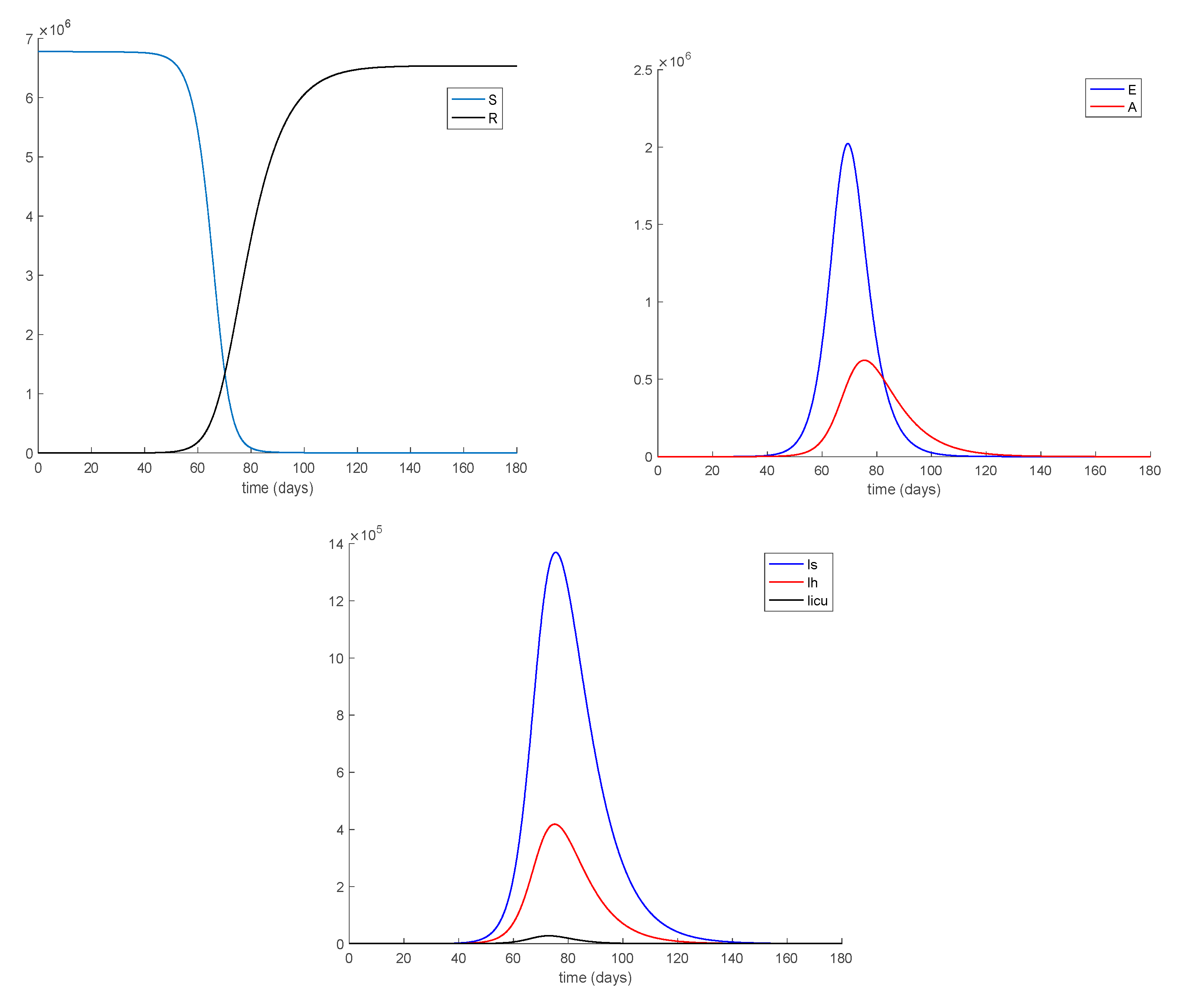
Example 1. Dynamics of the model in the absence of external actions.
Figure 1 displays the evolution of all populations in the absence of external control actions. It is observed in
Figure 1 that the model solution is well-defined and nonnegative as Theorem 2 states. It is also concluded from
Figure 1 that all the population would end up suffering from Covid-19 while the peak of hospitalized and ICU individuals will reach the values of 418,000 and 27,545, respectively. Thus, if no control action was taken then the health system resources (number of available beds) would be overflown. To avoid this situation, three control actions, namely vaccination, treatment, and control of the transmission rate through social distancing and other measurements, are considered and analyzed in the sequel.
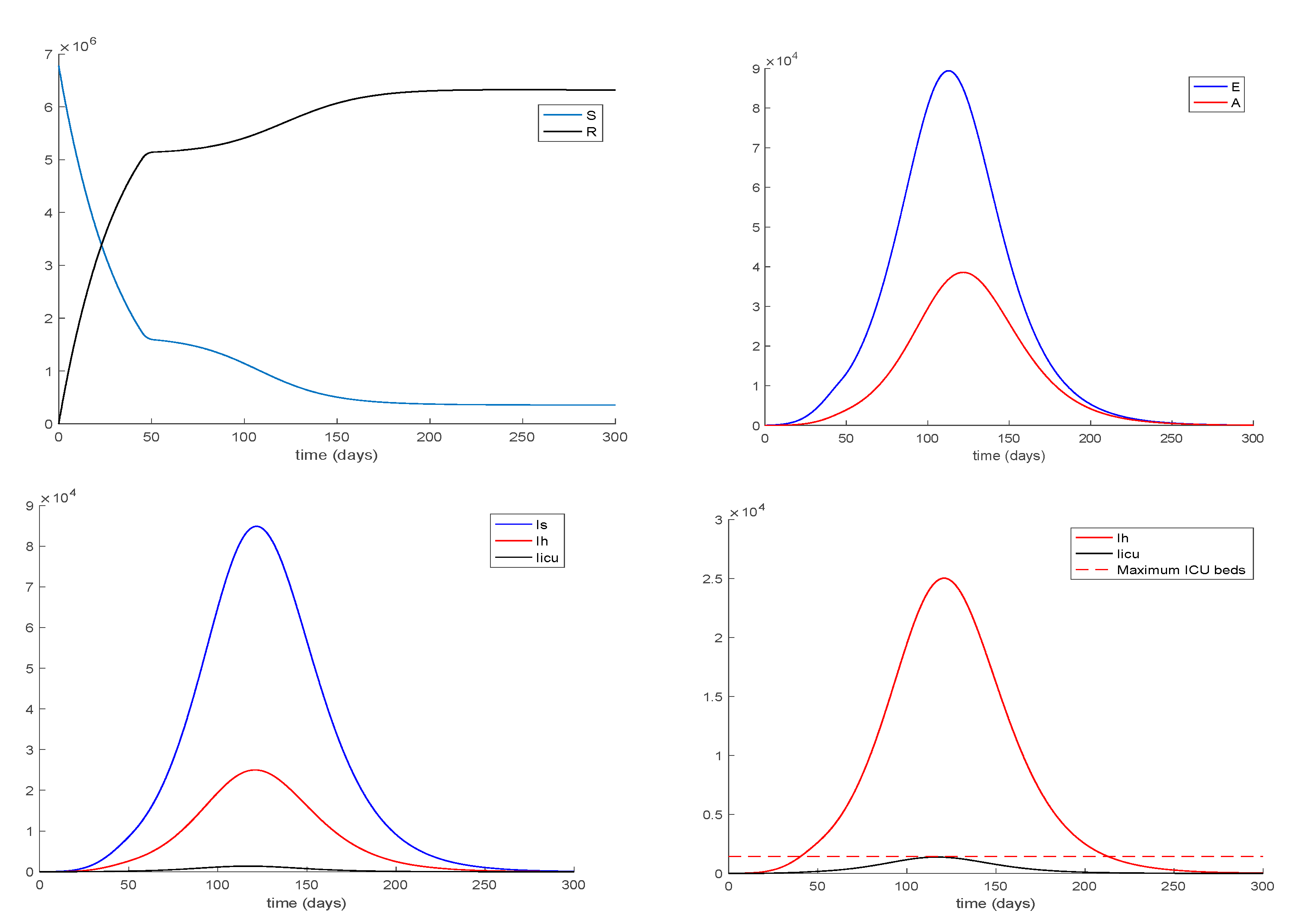
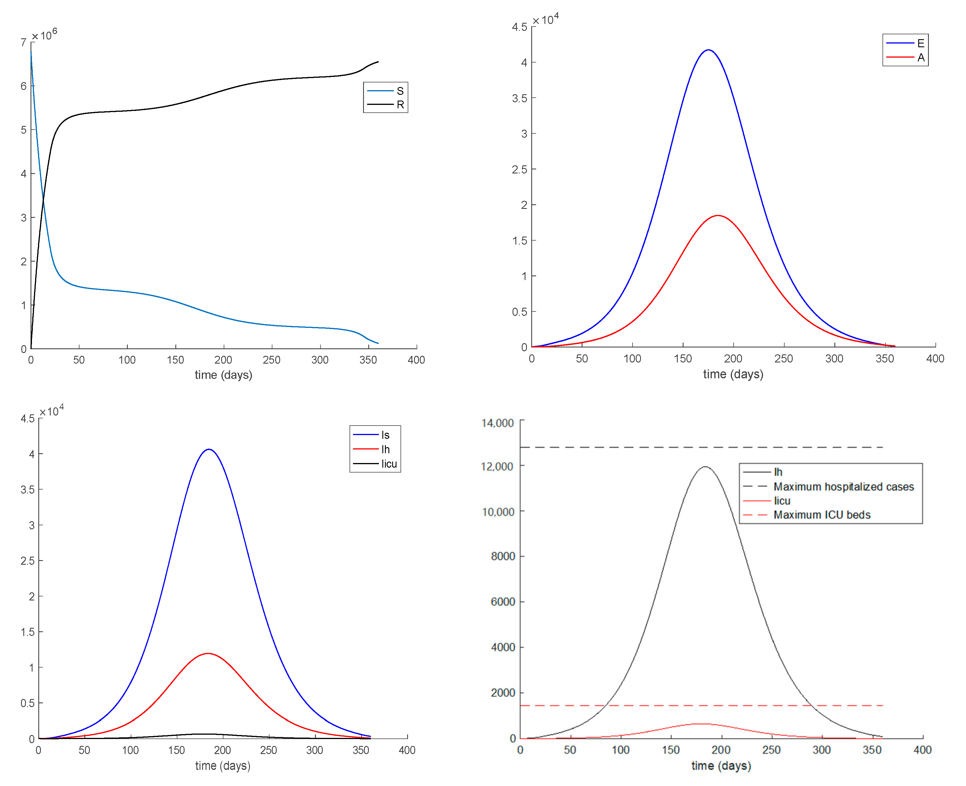
Example 2. Dynamics of the controlled model when Programme 2 is employed and the transmission rate is constant (i.e., it is not a manipulated control variable).
Now, Programme 2 given in
Section 4 is used with no iterations (i.e.,
) and
to design the external counteracting measurements in order to avoid the spread of COVID-19 while particularly guaranteeing that the number of individuals in ICU does not overflow the maximum available resources.
Figure 2 depicts the evolution of all subpopulations when this algorithm is employed with the transmission rate being kept constant, that is, it is not a control variable to be designed.
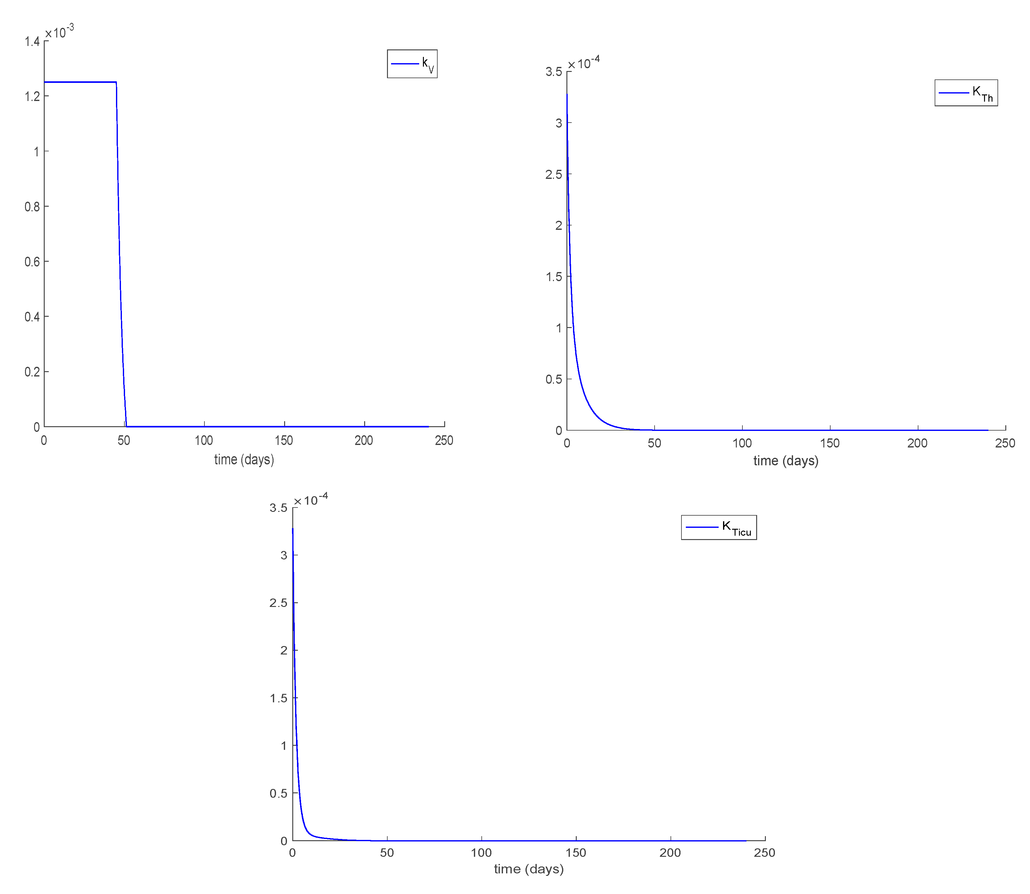
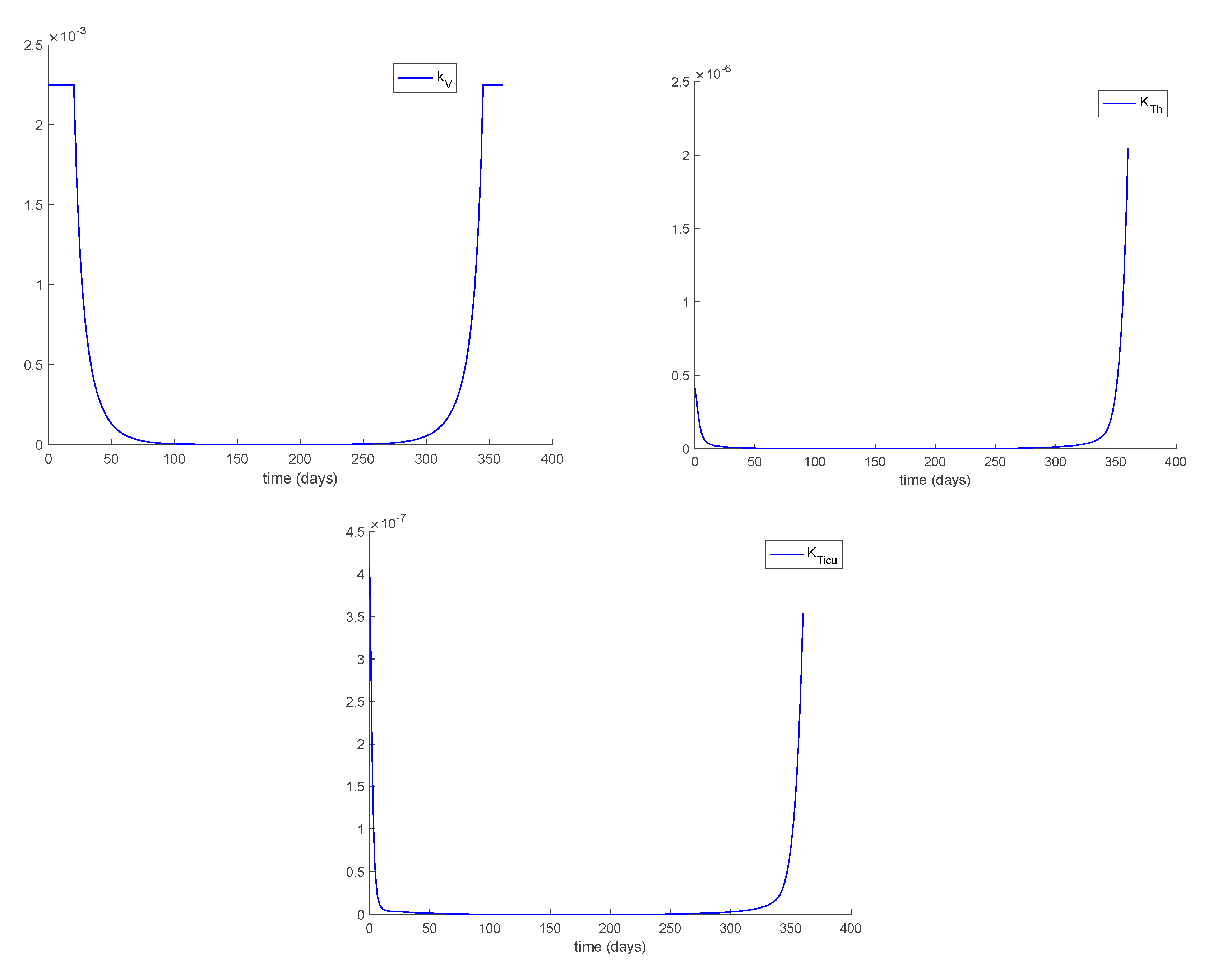
Figure 3 and
Figure 4 display the control gains and the control effort, respectively. The peak of hospitalized and ICU individuals reach the values of 25,830 and 1431, respectively.
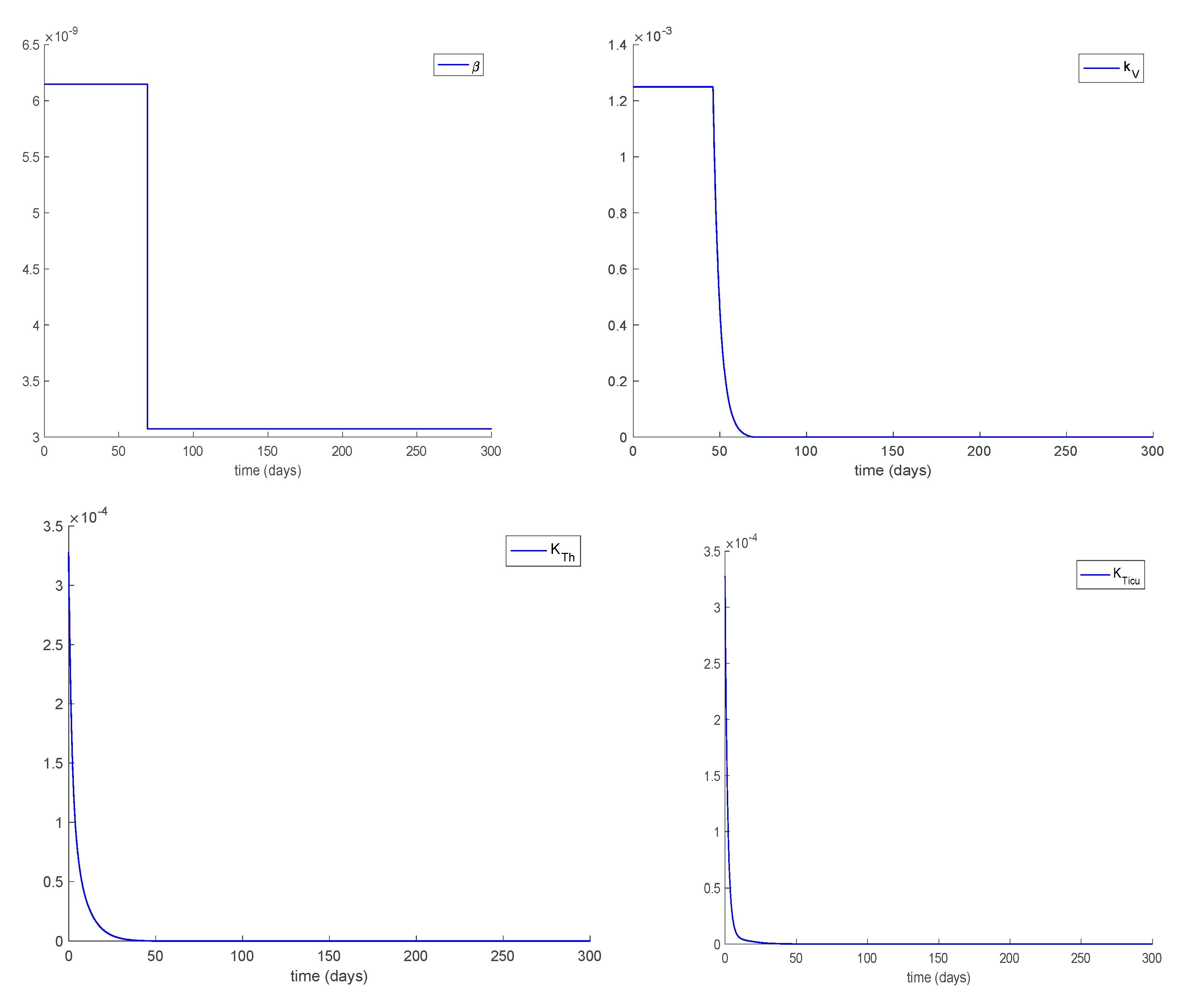
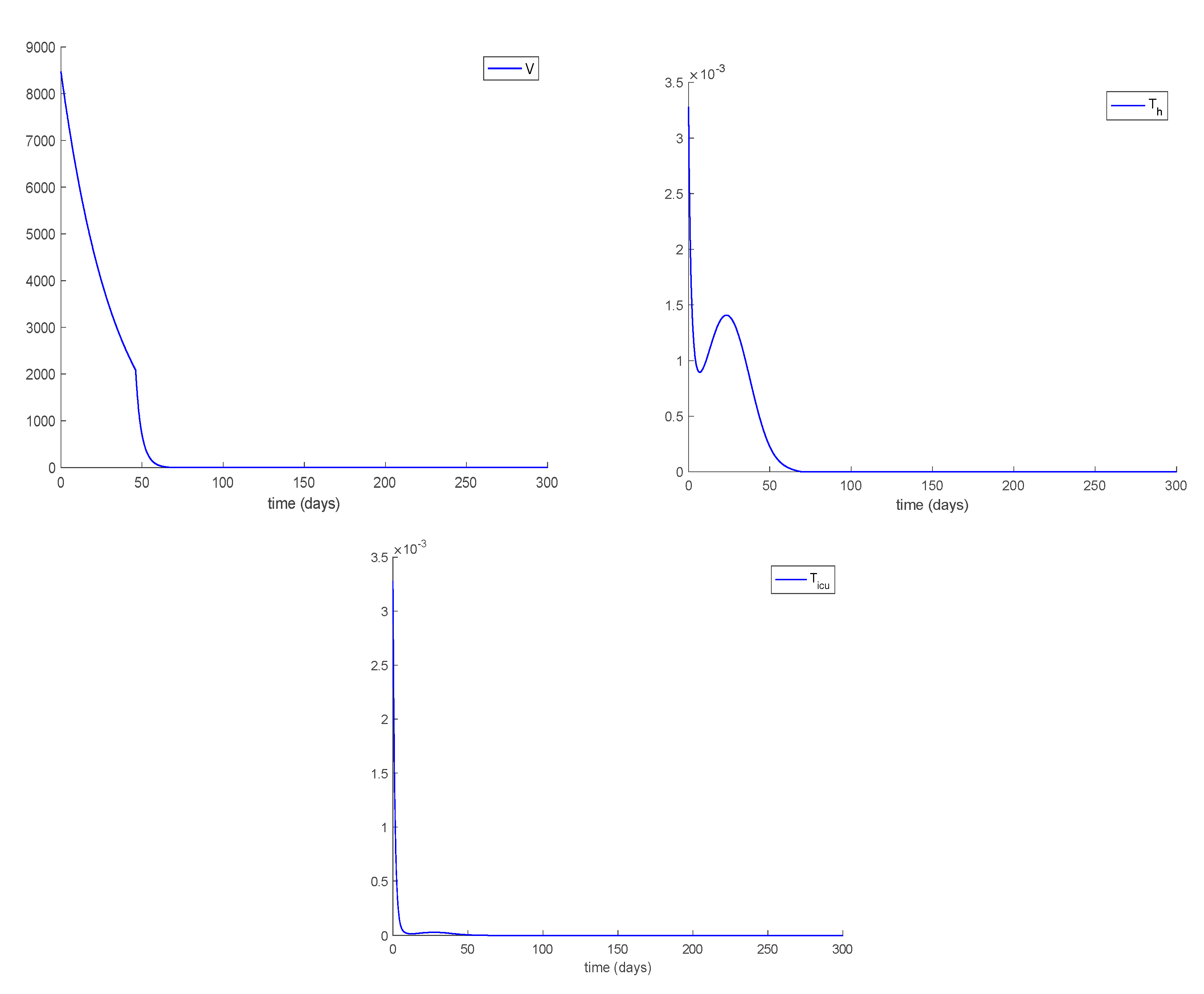
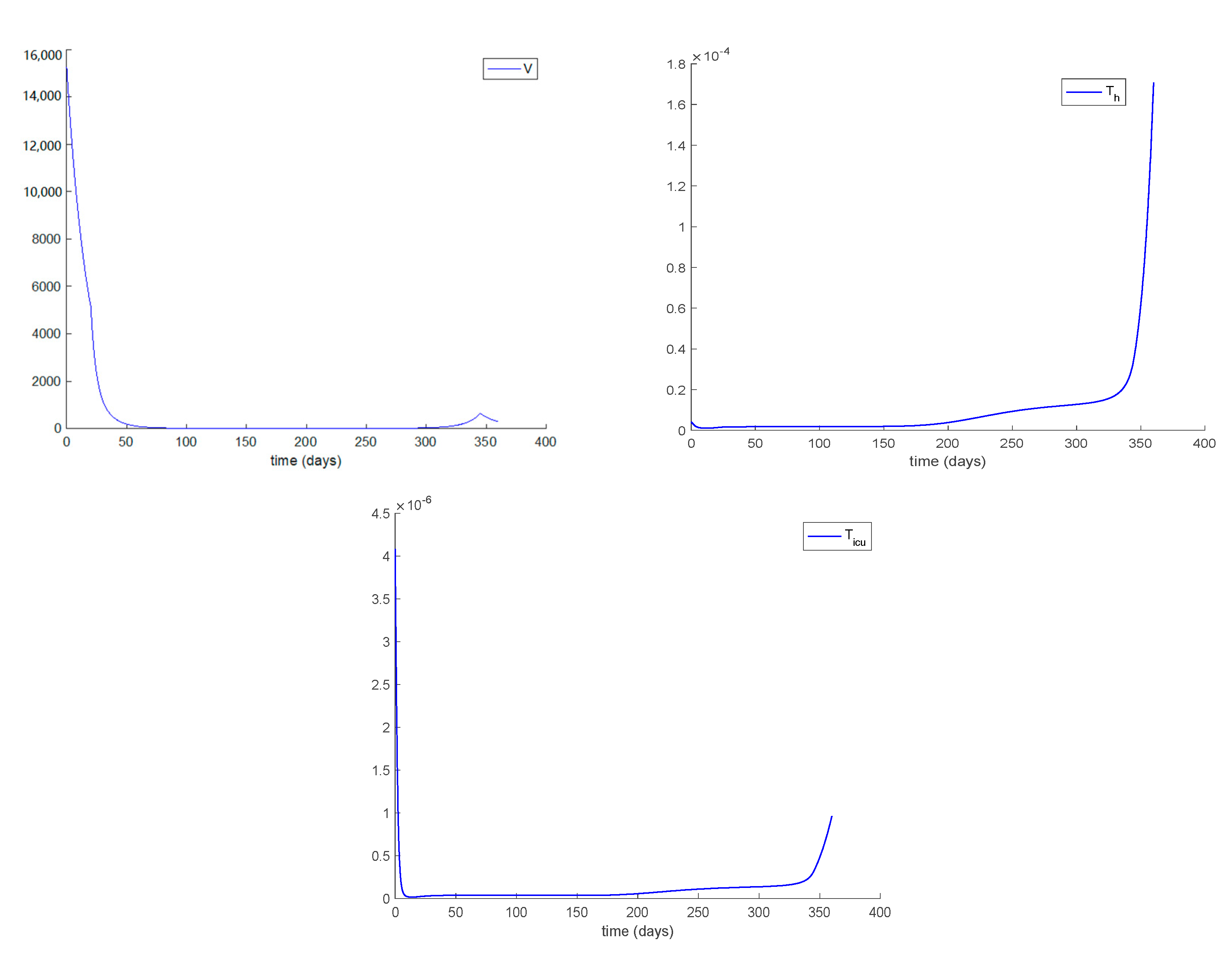
Example 3. Dynamics of the controlled model when Programme 2 is employed and the transmission rate is indeed a manipulated control variable.
The previous Example 2 did not consider the transmission rate as a control variable. Now, the case when
is also designed by the control algorithm is considered. Thus,
Figure 5 displays the evolution of the system through time when the transmission rate is also a control variable. The vaccination and treatment control gains are saturated to
and
, respectively and they are displayed in
Figure 6 while the corresponding control efforts are displayed in
Figure 7. The peak of hospitalized and ICU individuals reach the values of 6238 and 374, respectively.
It is observed a substantial reduction in the number of hospitalized cases in
Figure 5 with respect to the levels of
Figure 1 while
Figure 2 shows that the population becomes immune faster than in the absence of control actions, as it could have been intuitively expected.
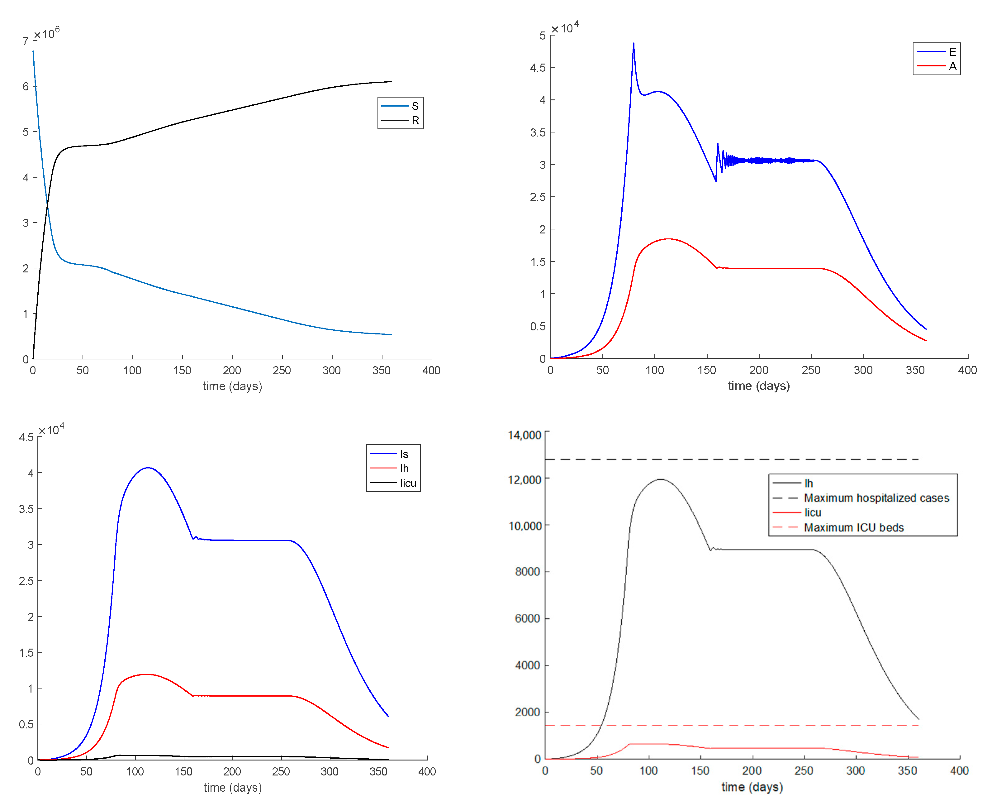
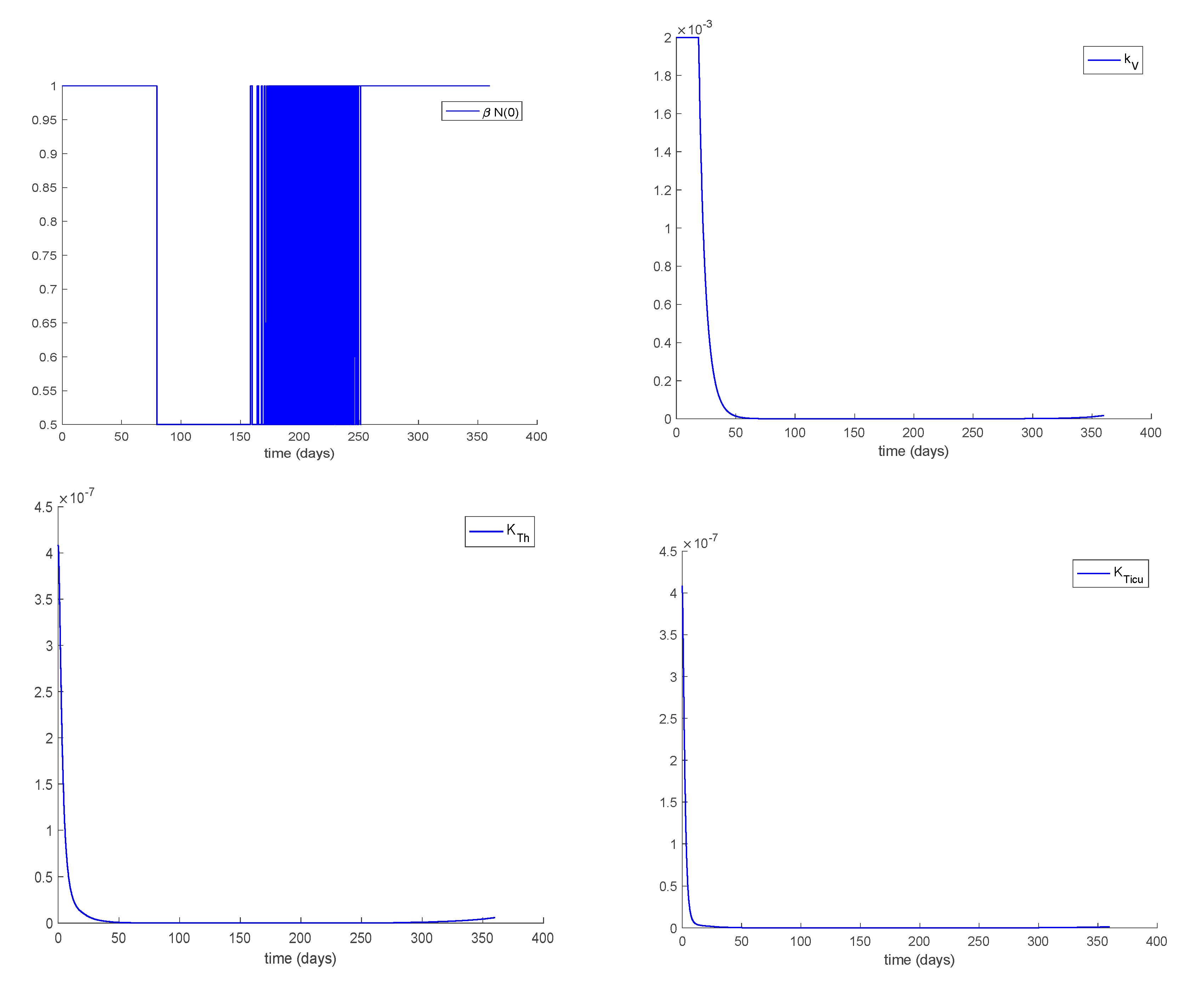
Example 4. Dynamics of the controlled model when Programme 6 is employed and the transmission rate is constant (i.e., it is not a manipulated control variable).
Figure 8,
Figure 9,
Figure 10 and
Figure 11 display some obtained results referred to the use of Programme 6 without iterations. The death toll is also reduced as concluded by comparing
Figure 2 and
Figure 8 regarding the evolution of the total population.
Figure 9 displays the vaccination and treatment control actions needed. The great improvement in the disease incidence is achieved at the expense of a high effort in vaccination as it is concluded from
Figure 4 and
Figure 10. As vaccination increases, the number of hospitalized cases declines. As claimed in
Section 3, the use of vaccination improves the behavior of the coronavirus spread. The peak of hospitalized and ICU individuals reach the values of 11,932 and 651, respectively.
Example 5. Dynamics of the controlled model when Programme 6 is employed and the transmission rate is indeed a manipulated control variable.
Finally,
Figure 11,
Figure 12 and
Figure 13 show the evolution of the system when Programme 6 is used, with
and
and without iteration, while beta is now a control variable. The value of
is constrained to the interval [0.5, 1] in order to capture the fact that the transmission rate cannot be reduced arbitrarily. The saturated lower bounds of the remaining control variables are fixed to zero. The proposed algorithm designs the control parameters so as to achieve the hospitalized and ICU constraints as it is observed in
Figure 11. As it is deduced by comparing
Figure 9 and
Figure 12, the vaccination effort reduces when the transmission factor beta is also employed as a control parameter. In this way, social distance, use of face masks, etc. can be used as effective control measurements, of course, at the expense of a very atypical lifestyle, as an alternative to vaccination in order to control the virus spreading. The peak of hospitalized and ICU individuals reach the values of 11,937 and 657, respectively.
It is of interest to give some discussion to the light of the comments in
Section 5 about how the intervention measures can be relevant to the achievement of the suitable disease transmission error when such a parameter is a control variable. In other words, the intervention measures might be weakened as the suitable targeted disease transmission rate as a control variable decreases and they should be more severe as such a value increases. Since the intervention measures contain chains of constraints on the social habits and uses, it is proposed the updating process of the measures over certain periods of time accordingly to the disease evolution. In particular, it is proposed the intervention measures updating every fifteen days by taking into account the average values of the transmission rate control values over such periods of time. The saturated averaged values of the disease transmission rate which calculated under Programme 5 in Example 5 are displayed in
Table 4. This averaging over longer periods of time has also a filtering effect on eventual oscillations between them maximum and minimum saturation values of the algorithms as it happens, for instance, with the transmission rate in
Figure 12 along the intermediate intervention time period.
Table 4 displays the average value of the transmission rate in fortnights provided by Programme 6 during the total simulation time of 360 days following the previous numerical results displayed in
Figure 11,
Figure 12 and
Figure 13. In particular, the suitable transmission rate obtained as a designed control variable via Programme 6 is displayed in the first plot of
Figure 12. It may be observed how the transmission rate varies between the two extreme values allowed by the control saturation for this control variable.
A brief discussion is now given about the mandatory use of masks and its removal at lunch/dinner time by considering it as the only intervention measure. The objective is to calculate the estimated average fraction of time per fortnight
of use of masks necessary to achieve the foreseen transmission rate which, together with the remaining calculated vaccination and treatment control components, achieves the suited infection tracking objective. It is assumed that the mask use (event
) is mandatory along a certain time period in average per day/individual and removed (event
) for another certain period of time per day/individual in social risk situations like, for instance, at bars or restaurants. The average degrees of fulfillments are assumed to be
and
, respectively, and the respective average degrees of effectiveness are assumed to be
and
,
and
with
, which corresponds to an average of
h per fortnight or
h per day if the masks should be used along 12 h per day. For simplicity, assume that
and that the saturated level
is related to the absence of intervention, that is, the use of masks is not mandatory related to the serious infection tolerated levels. This gives
for the corresponding fortnight. As a result,
Table 4 gives the following values for each fortnight after using the formula:
which yields:
These above values can easily translated into hours of masks use per day along the fortnight with 12 h corresponding to .
7. Conclusions and Potential Future Research
This paper has developed a so-called SE(Is)(Ih)(Icicu)AR epidemic model which includes four infectious subpopulations which are the asymptomatic one, the slight one, the hospitalized one which does not need intensive care, that which needs intensive care. The model is discussed under four different controls which are vaccination, differentiated treatment control for the hospitalized infectious both outside and within the intensive care unit and the eventual design of the allowed maximum levels of the disease transmission rate contagious contacts depending on the strongness, or even forcefulness, degree (from significantly weak to very strong) of public intervention decisions. The two subpopulations of hospitalized infectious patients define the measurable outputs of the model which can be dealt with individually, that is as two different output components, or jointly if the output is defined as the sum of both populations. Also, the output can be defined just as a single function associated to the patients staying at the intensive care unit. The various definitions of the output might be chosen optionally. The feedback controls are updated so that the levels of infection are under certain maximum allowed upper-bounds so as to satisfy the hospital capacity of patients admission and their effective treatment. The control gains are designed along previous time intervals so that the mentioned allowed levels are respected at certain testing time sampling instants. Several control synthesis algorithms have been given depending on the particular definition used in each case for the measurable output. The proposed model and its output controllability issues together with its above mentioned corresponding control synthesis algorithms have been tested through examples based on parameterizations of the COVID-19 pandemic.
A future research of interest is to incorporate the estimation of the transmission rate bounds to their introduction in the algorithms by using recorded experimental data values which take into account the restrictions in the various phases of the intervention measures. Such restrictions to consider are, for instance, effects of partial or total confinement rules, mobility limitations, mandatory use of masks, maximum private, social and collective meeting attendance constraints, etc. It is also of relevant interest to incorporate the vaccination efficiency percentage in the model analysis when such vaccines become ready for distribution and their application is expected within months. Those efficiency percentages might be incorporated as a fixed factor, or including an eventual variation range, to the vaccination control gains. In that way, it could be compared how the vaccines, with their estimated efficiency ranges, could decrease the infection data by comparing the obtained data under vaccination to the registered official values for the previous evolution stages of the pandemic spread. The idea could also be extended to the use of other controls like the decreasing of the transmission rate via the application of certain rules or social distance, use of masks, etc.
Another point of interest for future research is the incorporation of appropriate stochastic analysis frameworks, incorporating, for instance, eventual perturbations to extend the results of this work to the stochastic case.


